Output Feedback-Based Neural Network Sliding Mode Control for Electro-Hydrostatic Systems with Unknown Uncertainties

Abstract

This paper proposes an output feedback-based control for uncertain electro-hydrostatic systems (EHSs) to satisfy high output tracking precision under the influences of unknown mismatched and matched uncertainties and unstructured dynamical behavior. In this configuration, an extended state observer (ESO) is first employed to obtain unmeasured states and suppress the adverse effect of matched uncertainty. Meanwhile, the influence of unstructured dynamical behavior is approximated by employing a radial basis function neural network (RBFNN)-based technique. With the unmeasured states observed, matched uncertainty, and system dynamics compensated, the robust backstepping sliding mode control is accordingly established and the lumped mismatched uncertainty is then suppressed through disturbance observer-based adaptive law. Interestingly, the proposed control methodology requires only output feedback but can address the whole system dynamics. The stability of the closed-loop system is theoretically proven through a Lyapunov theorem and the effectiveness of the proposed methodology is demonstrated through comparative simulations.

1. Introduction

Achieving control accuracy for electro-hydrostatic pump-controlled systems (EHPSs) has triggered an interesting topic and has broadly been studied for the past decade. With the advantages of light weight, high force/torque density, high mobility and reliability, and ease of maintenance, the EHPS has become a core actuation component of numerous modern hydro-mechanical applications such as aviation [1], wheel-legged robots [2], exoskeleton robots [3,4], articulated manipulators [5], renewable energy [6,7,8], and so forth [9,10,11,12,13]. Especially, high efficiency can be achieved compared to the electro-hydraulic servo-valve-control type actuators (EHSAs), which have throttling loss due to the servo-valve dynamical behavior. Nonetheless, inherent fluid properties, nonlinearity, modeling error, bypass friction, leakage, unknown external disturbance, and unstructured uncertainties adversely affect the control accuracy. Moreover, unmeasured states also bring an obstacle to achieving robust control developments.

Of a simple calculation with only output required, the traditional model-free proportional–integral–derivative (PID) control has widely been exploited for various industrial applications. Later, variations such as adaptive PID, fuzzy PID, fractional PID, particle swarm optimization, genetic algorithms, other optimization-based adaptive PID control, learning-based control, and so forth have favorably been developed for EHPSs [14,15,16,17]. Regarding the introduced literature, the tracking performance was improved, as the controller gains adapted to satisfy specific working conditions compared to the previous studies. However, the system dynamics were neglected and the effects of disturbance and internal uncertainties have not been tackled, which has raised an arduous challenge to achieve robust tracking qualification against perturbation and uncertainties.

Compared to the model-free strategies [14,15,16,17], the model-based control method is considered a feasible solution to deal with the system model. Among various methodologies, backstepping control (BSC) and sliding mode control (SMC) have been used as powerful tools that can not only deal with the system dynamics but also guarantee the closed-loop system stability for the required control satisfaction. The BSC possesses the advantage of guaranteeing closed-loop stability through a recursive process; however, this also brings burdensome computations and complexity explosion in the case of high-order systems. Meanwhile, the SMC has the merits of reducing the system order and robustness against perturbation; yet it is vulnerable to the influence of internal uncertainties. Reasonably, the integration of backstepping SMC (BSMC) takes advantage of both BSC and SMC and has been broadly exploited to derive control action for diverse applications such as hydraulic manipulators [18,19,20], construction machines [21], and so forth. Additionally, observer-based control was also hybridized to cope with the unknown disturbances and uncertainties [5,22,23,24]. In [5], Lee et al. proposed dual disturbance observers (DOs) to compensate for the friction impact and suppress undesirable internal leakage. In [22], Ba et al. conducted high-order disturbance observer (DO)-based control for force and pressure dynamics of an EHPS to mitigate the impacts of disturbance and uncertainties. In [23], Trinh et al. employed a hybrid disturbance observer (DO)–extended state observer (ESO) to mitigate the influences of external load disturbance and internal leakage in EHPSs. Subsequently, a BSMC was designed to achieve satisfactory control and output performance. In [24], the authors examined an EHPS-driven hydraulic crane and established an ESO-based integral BSMC to regulate the output position performance under time-varying load disturbance. Various contributions have been published [25,26]; however, they require full state feedback for the control and adaptive law implementations.

Following up on the output feedback-based control, the authors in [27] proposed an ESO-based output feedback control for the EHSA type. The observability of the proposed algorithm was demonstrated by experiments where good output tracking regulation with well-estimated unmeasurable states (velocity and uncertainties) was accomplished. Inheritably, output feedback-based adaptive disturbance rejection controls (ADRCs) were developed based on the core of ESO [28,29]. In [30], Tran et al. studied an extended high-gain observer-based SMC for the EHPS rotary type subject to variant payload, unknown friction, and uncertainties. The effectiveness of the method was examined through comparative experiments. However, only matched uncertainties were pointed out. Following this shortcoming, Nguyen et al. developed an output feedback-based BSMC with an extended sliding mode observer proposed for an EHPS to comprehensively clarify the undesired effects of external load and internal leakage [31]. Considering constraints, the authors in [32] integrated input saturation into a model-based control to prevent the control signal from being singular due to the discontinuity of the saturated signal. Despite good results, the authors investigated EHPS models with well-known dynamical terms in the mentioned works. Thereby, unknown disturbances and uncertainties, including internal leakage, parametric uncertainty, unmodeled nonlinearity terms, and modeling errors, were lumped and suppressed using an observer-based control scheme. Practically, it is quite difficult to exactly identify the system’s dynamics due to long-term usage and degradation.

Known as an effective technique to deal with smooth functions, universal approximation engines such as a fuzzy logic mechanism or radial basis function neural network (RBFNN)-based methods have been intensively incorporated into the control synthesis to approximate dependent-state functions. The potential of using intelligence-based control has been validated through both simulations and experiments for general nonlinear systems [33,34,35]. Within the scope of EHPSs, the authors in [19] employed the RBFNN-based technique to approximate the modeling error of a hydraulic manipulator. In [36], Phan et al. made use of the RBFNN to eliminate the adverse impact of mismatched disturbance. Similarly, the authors in [37] combined the RBFNN to reduce the influence of the time-delayed estimation error when initializing the control action for cable-driven manipulators. The feasibility of the RBFNN has been persuasively studied through numerous studies; nevertheless, to the best of our knowledge, the inclusion of RBFNNs and observers to suppress the unstructured dynamics and uncertainties and facilitate the output feedback control has not been reported elsewhere.

Summing the above research gaps, this paper aims to propose a robust output feedback-based neural network backstepping sliding mode control (OF-NBSMC) for an uncertain EHPS, subject to unknown disturbance, uncertainties, and unstructured dynamics, to meet the designated reference trajectory. The proposed method is established based on integrating estimators and RBFNN-based approximators to comprehensively address the above systematic problems. In brief, the paper contributions are as follows:

• Proposing a robust OF-NBSMC for uncertain EHPSs subject to unknown load disturbance, friction, matched uncertainty, and unstructured dynamical behavior.
• With only output available, an ESO is first employed to help observe other unmeasured states and suppress the influence of matched uncertainty.
• Conducting an RBFNN-based approximation integrated with a disturbance observer (DO)-based adaptive law to decouple the dynamical behavior of the mechanical part with the impact of load disturbance to satisfy specific working requirements.
• The system stability is theoretically proven and the feasibility of the proposed methodology is verified through comparative simulations.

The rest of the paper is organized as follows. Section 2 formulates the general model of an EHPS with the necessary hypothesis to facilitate the proposed control manipulation. In Section 3, estimators and approximation operators are presented to observe unmeasurable states. Accordingly, in Section 4, the robust OF-NBSMC is formulated with the closed-loop system stability guaranteed through the Lyapunov theorem. The feasibility of the proposed control algorithm is then examined through comparisons in Section 5. Finally, Section 6 summarizes key techniques and is a prominence for further development.

2. Problem Formulation

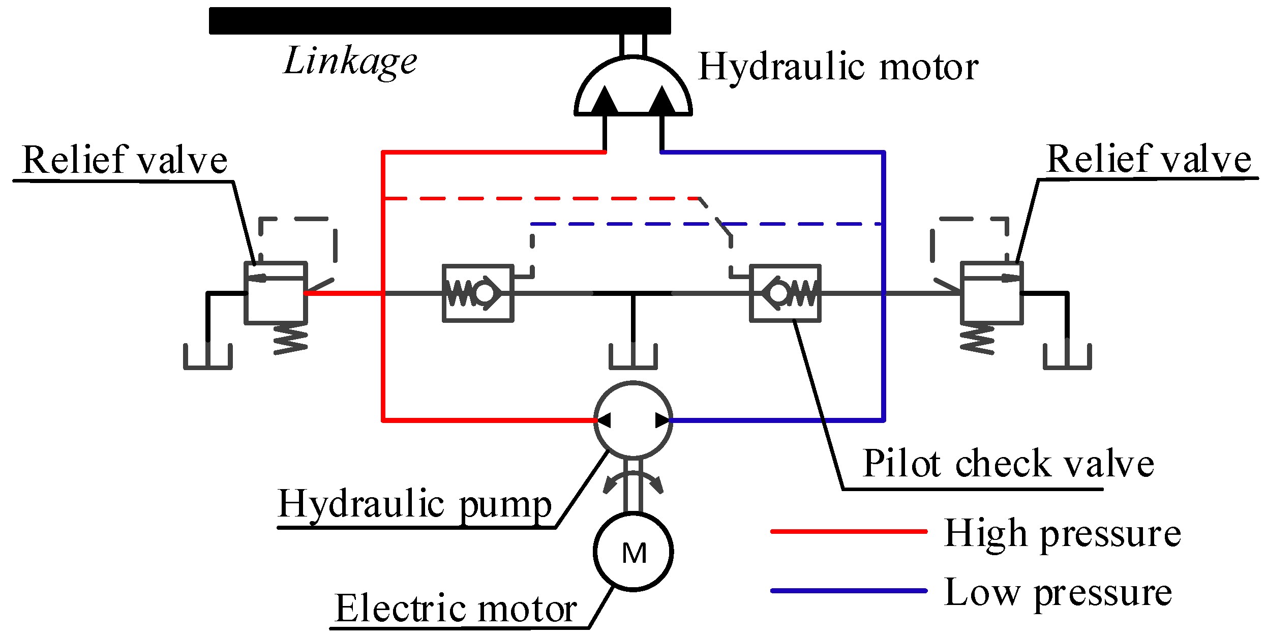
2.1. System Descriptions

A detailed schematic of the EHPS can be referred to in [23,31]. Within normal working operation, i.e., without faults or failures, the dynamical behaviors of some components, such as check valves, relief valves, filters, and so forth, could be ignored since the pressure inside pipelines and actuator chambers should not exceed the setting of maximum pressure of the relief valve. However, those components have some impacts, even though they are small. Thus, they are considered modeling errors or uncertainties [31]. Therefore, in this paper, a simplified specific EHPS is considered as shown in Figure 1.

In brief, the EHPS comprises a hydraulic pump, driven by an electric motor, to pressurize and run the hydraulic motor with a linkage mounted at the output shaft. Two relief valves are equipped to protect the system from over-pressure by releasing flow to the oil tank. And pilot check valves are to support the flow of hydraulic oil to the circuit in the case of low pressure by sucking oil from the tank.

The dynamical behavior of the mechanical part is modeled based on Newton’s second law as

$$J\ddot{\varphi }+{\tau }_{fr}\left(\varphi ,\dot{\varphi }\right)+{\tau }_{ext}={\tau }_{act},$$

(1)

where J denotes the inertial moment of the rotary actuator; $\varphi ,\dot{\varphi }$, and $\ddot{\varphi }$ represent the actuator’s angular position, angular velocity, and acceleration, respectively; ${\tau }_{fr}$ reflects the poorly known friction; ${\tau }_{ext}$ represents the unknown external load; and ${\tau }_{act}$ is the active torque to drive the actuator, whose expression is:

$${\tau }_{act}=A_{\omega }\left(P_1-P_2\right),$$

(2)

with $A_{\omega }$ being the radiant displacement and $P_1$ and $P_2$ being pressures in two chambers.

The dynamics of pressures $P_1$ and $P_2$ is derived based on the hydraulic continuity equations:

$$\left\{\begin{array}{l}{\displaystyle \frac{d{P}_1}{dt}}={\displaystyle \frac{\beta }{V_1}}\left(+D_P{\Omega }_P-A_{\omega }\dot{\varphi }-Q_{in-leak}\left(P_1,P_2\right)-Q_{rv}\right)\\ {\displaystyle \frac{d{P}_2}{dt}}={\displaystyle \frac{\beta }{V_2}}\left(-D_P{\Omega }_P+A_{\omega }\dot{\varphi }+Q_{in-leak}\left(P_1,P_2\right)-Q_{rv}\right)\end{array}\right.,$$

(3)

where β is the effective bulk modulus; $V_1=V_{10}+A\varphi$ and $V_2=V_{20}-A\varphi$ are total volumes of two chambers with $V_{01}$ and $V_{02}$ being the initial volume, including the volumes of pipelines, when the actuator is in the neutral position; $D_P$ represents the pump displacement; ${\Omega }_P$ is the controlled pump speed; $Q_{in,leak}\left(P_1,P_2\right)$ is the unknown internal leakage; and $Q_{rv}$ is the flow through the safety relief valve.

By first subtracting the first sub-equation and second sub-equation in (3), then multiplying the obtained result with $A_{\omega }/J$, one has:

$$\begin{array}{l}{\displaystyle \frac{A_{\omega }\left({\dot{P}}_1-{\dot{P}}_2\right)}{J}}=\left({\displaystyle \frac{1}{V_1}}+{\displaystyle \frac{1}{V_2}}\right){\displaystyle \frac{\beta A_{\omega }{D}_P{\Omega }_P}{J}}-\left({\displaystyle \frac{1}{V_1}}+{\displaystyle \frac{1}{V_2}}\right){\displaystyle \frac{\beta A_{\omega }^2}{J}}\dot{\gamma }\\ \hspace{0.17em}\hspace{0.17em}\hspace{0.17em}\hspace{0.17em}\hspace{0.17em}\hspace{0.17em}\hspace{0.17em}\hspace{0.17em}\hspace{0.17em}\hspace{0.17em}\hspace{0.17em}\hspace{0.17em}\hspace{0.17em}\hspace{0.17em}\hspace{0.17em}\hspace{0.17em}\hspace{0.17em}\hspace{0.17em}-{\displaystyle \frac{\beta A_{\omega }}{J}}\left({\displaystyle \frac{1}{V_1}}+{\displaystyle \frac{1}{V_2}}\right)Q_{in-leak}\left(P_1,P_2\right)+{\displaystyle \frac{\beta A_{\omega }}{J}}\left(-{\displaystyle \frac{1}{V_1}}{Q}_{rv1}+{\displaystyle \frac{1}{V_2}}{Q}_{rv2}\right)+{\delta }_{\mathrm{modeling}}\end{array},$$

(4)

It is noted that the system should be operated such that the pressure inside should not exceed the maximum setup values of the relief valves (normal operation). Subsequently, to simplify the modeling, there is no flow through the relief valves in this case. Thereby, the dynamics of relief valves can be ignored. However, there may exist a small flow through valves due to the orifice; thus, it is reasonable to expect the existence of small ${\tilde{Q}}_{rv1}={\tilde{Q}}_{rv2}\approx 0$ along with the modeling errors and leakage.

By setting ${\left[x_1,x_2,x_3\right]}^T={\left[\varphi ,\hspace{0.17em}\hspace{0.17em}\dot{\varphi },\hspace{0.17em}\hspace{0.17em}{A}_{\omega }\left(P_1-P_2\right)/J\right]}^T$, the dynamical model of a specific EHPS can be expressed as

$$\left\{\begin{array}{l}{\dot{x}}_1=x_2\\ {\dot{x}}_2=f_2\left(x_1,x_2\right)+x_3+{\delta }_2\\ {\dot{x}}_3=f_3\left(x_1,x_2,x_3\right)+g_3\left(x_1\right)u+{\delta }_3\\ y=x_1\end{array}\right.,$$

(5)

where y is the output, u is the input voltage; $f_2\left(x_1,x_2\right)=-{\displaystyle \frac{1}{J}}{\tau }_{fr}\left(x_1,x_2\right)$, ${\delta }_2=-{\displaystyle \frac{1}{J}}{\tau }_{ext}$, $f_3\left(x_1,x_2\right)=-\left({\displaystyle \frac{1}{V_1}}+{\displaystyle \frac{1}{V_2}}\right){\displaystyle \frac{\beta A_{\omega }^2}{J}}\dot{\varphi }-{\displaystyle \frac{\beta A_{\omega }}{J}}\left({\displaystyle \frac{1}{V_1}}+{\displaystyle \frac{1}{V_2}}\right)Q_{in-leak}\left(P_1,P_2\right)$, $g_3\left(x_1\right)=\left({\displaystyle \frac{1}{V_1}}+{\displaystyle \frac{1}{V_2}}\right){\displaystyle \frac{\beta A_{\omega }{D}_P{k}_P}{J}}$ with the pump coefficient $k_P$ representing the proportional ratio between the pump speed ${\Omega }_P$ and control signal u, and ${\delta }_3={\displaystyle \frac{\beta A_{\omega }}{J}}\left(-{\displaystyle \frac{1}{V_1}}{\tilde{Q}}_{rv1}+{\displaystyle \frac{1}{V_2}}{\tilde{Q}}_{rv2}\right)+{\delta }_{\mathrm{modeling}}$.

Assumption 1.

The pump dynamics and electrical part operate without faults and are delayed. Thus, the pump speed is proportional to the control signal u [23,31]. The detailed dynamical model between the pump speed and control signal u will be investigated in future works.

As seen, it is a challenge to conduct an output feedback control when the structures of $f_2\left(x_1,x_2\right)$, ${\delta }_2$, $f_3\left(x_1,x_2,x_3\right)$, ${\delta }_3$ are not well modeled and parameterized. Moreover, the influences of dynamics terms $f_2\left(x_1,x_2\right)$ and ${\delta }_2$ need to be decoupled as they appear in the same channel. In this manner, the dynamical behavior $f_2\left(x_1,x_2\right)$ is approximated using the RBFNN while ${\delta }_2$ is estimated using an observer. Furthermore, within this research, the effects of $f_3\left(x_1,x_2,x_3\right)$ and ${\delta }_3$ need not be decoupled; hence, they are reasonably lumped into F₃. As a result, system (5) becomes:

$$\left\{\begin{array}{l}{\dot{x}}_1\left(t\right)=x_2\left(t\right)\\ {\dot{x}}_2\left(t\right)=f_2\left(x_1,x_2,t\right)+x_3\left(t\right)+{\delta }_2\left(t\right)\\ {\dot{x}}_3\left(t\right)=F_3\left(x_1,x_2,x_3,t\right)+g_3\left(x_1,t\right)u\end{array}\right.,$$

(6)

2.2. Preliminaries

The goal is to manipulate the output y to track a required reference y_d. To facilitate the control design, the following assumptions are utilized:

Assumption 2 [38].

The desired trajectory y_d and its first derivative ${\dot{y}}_d$ are continuous and bounded.

Assumption 3 [39].

Mismatched disturbance ${\delta }_2\left(t\right)$ and its first derivative ${\dot{\delta }}_2\left(t\right)$ are bounded by unknown constants, i.e., $\left|{\delta }_2\left(t\right)\right|\le D_2$ and $\left|{\dot{\delta }}_2\left(t\right)\right|\le {\Delta }_2$.

Assumption 4 [23].

$f_2\left(x_1,x_2,t\right)$ is unknown but smooth and bounded. Moreover, it is Lipschitz with respect to corresponding states.

Assumption 5.

Regarding the system characteristics, unknown dynamical terms $f_2\left(x_1,x_2,t\right)$ and $F_3\left(x_1,x_2,x_3,t\right)$ with their first derivatives ${\dot{f}}_2\left(x_1,x_2,t\right)$ and ${\dot{F}}_3\left(x_1,x_2,x_3,t\right)$ are bounded by unknown upper constants, i.e., $\left|f_2\left(x_1,x_2,t\right)\right|\le {\overline{f}}_2^c$, $\left|F_3\left(x_1,x_2,x_3,t\right)\right|\le {\overline{F}}_3^c$, $\left|{\dot{f}}_2\left(x_1,x_2,t\right)\right|\le {\overline{f}}_2^d$, and $\left|{\dot{F}}_3\left(x_1,x_2,x_3,t\right)\right|\le {\overline{F}}_3^d$.

Remark 1.

The validity of Assumptions 4 and 5 comes from the fact that external disturbances and $f_2\left(x_1,x_2,t\right)$ are all physically bound. Without loss of generality, $f_2\left(x_2\right)$ is a function of the actuator position and velocity [6] that is always constrained regarding the working range and system specifications. Meanwhile, the external disturbance relates to the system’s workability and should not exceed its maximum workload as the safety criterion. It also requires a certain transient time to impact the system’s behavior.

Lemma 1 [34].

In view of Young’s inequality, the following result holds:

$$xy\le {\displaystyle \frac{{\vartheta }^a}{a}}{\left|x\right|}^a+{\displaystyle \frac{1}{b{\vartheta }^b}}{\left|y\right|}^b,$$

(7)

with ϑ > 0 and ${\displaystyle \frac{1}{a}}+{\displaystyle \frac{1}{b}}=1$. In this paper, a = b = 2 is selected to simplify the control parameters’ selection, and ϑ is arbitrarily selected to achieve flexible choice for the observer and updating gains for estimating unknown unstructured dynamical terms $f_2\left(x_1,x_2,t\right)$, $F_3\left(x_1,x_2,x_3,t\right)$, and disturbance ${\delta }_2\left(t\right)$.

In addition, hereafter, $f_2\left(x_1,x_2,t\right)$, ${\delta }_2\left(t\right)$, $F_3\left(x_1,x_2,x_3,t\right)$, $g_3\left(x_1,t\right)$ are, in turn, shortened as $f_2\left(x_1,x_2\right)$, ${\delta }_2$, $F_3$, and $g_3$ for simplicity.

3. Observer and Approximation Mechanisms

In this manuscript, the unknown terms ${\delta }_2\left(t\right)$ and $F_3\left(x_1,x_2,x_3,t\right)$ are viewed as extended states and thus estimated using extended state observers. Meanwhile, the state-dependent dynamics $f_2\left(x_1,x_2,t\right)$, which includes poorly known parameters of the mechanical part (friction), is approximated using the RBFNN. The proposed control scheme is depicted in Figure 2.

Let $x_{e1}={\delta }_2\left(t\right)$ be the mismatched disturbance and $x_{e2}=F_3\left(x_1,x_2,x_3,t\right)$ be the extended state of matched uncertainty, then the equivalent system (6) can be rearranged as

$$\left\{\begin{array}{l}{\dot{x}}_1=x_2\\ {\dot{x}}_2=f_2\left(x_1,x_2\right)+x_3+x_{e1}\\ {\dot{x}}_3=g_3\left(x_1\right)u+x_{e2}\\ {\dot{x}}_{e2}=\rho \end{array}\right.,$$

(8)

3.1. Observer-Based Matched Uncertainty Suppression

In view of the extended state observer [27], the unknown mismatched disturbance x_e1 and matched uncertainty x_e2 are estimated as follows:

$$\left\{\begin{array}{l}{\dot{\widehat{x}}}_1={\widehat{x}}_2\hspace{0.17em}\hspace{0.17em}\hspace{0.17em}\hspace{0.17em}\hspace{0.17em}\hspace{0.17em}\hspace{0.17em}\hspace{0.17em}\hspace{0.17em}\hspace{0.17em}\hspace{0.17em}\hspace{0.17em}\hspace{0.17em}\hspace{0.17em}\hspace{0.17em}+4\alpha \left(x_1-{\widehat{x}}_1\right)\hspace{0.17em}\\ {\dot{\widehat{x}}}_2={\widehat{x}}_3+f_2\left({\widehat{x}}_1,{\widehat{x}}_2\right)\hspace{0.17em}+6{\alpha }^2\left(x_1-{\widehat{x}}_1\right)\\ {\dot{\widehat{x}}}_3=g_3\left(x_1\right)u+{\widehat{x}}_{e2}\hspace{0.17em}\hspace{0.17em}\hspace{0.17em}+4{\alpha }^3\left(x_1-{\widehat{x}}_1\right)\\ {\dot{\widehat{x}}}_{e2}=\hspace{0.17em}\hspace{0.17em}\hspace{0.17em}\hspace{0.17em}\hspace{0.17em}\hspace{0.17em}\hspace{0.17em}\hspace{0.17em}\hspace{0.17em}\hspace{0.17em}\hspace{0.17em}\hspace{0.17em}\hspace{0.17em}\hspace{0.17em}\hspace{0.17em}\hspace{0.17em}\hspace{0.17em}\hspace{0.17em}\hspace{0.17em}\hspace{0.17em}\hspace{0.17em}{\alpha }^4\left(x_1-{\widehat{x}}_1\right)\end{array}\right.,$$

(9)

where α is a positive constant; ${\widehat{x}}_i$ (i = 1, 2, 3) are estimated states of $x_i$; ${\widehat{x}}_{e1}$ and ${\widehat{x}}_{e2}$ are the estimations of $x_{e1}$ and $x_{e2}$, respectively. Since $f_2\left(x_1,x_2\right)$ and $g_3\left(x_1\right)$ are Lipchitz, the following inequalities are attained [33]:

$$\left|{\psi }_2\right|=\left|f_2\left(x_1,x_2\right)-f_2\left({\widehat{x}}_1,{\widehat{x}}_2\right)\right|\le {\sigma }_{f1}\left|x_1-{\widehat{x}}_1\right|+{\displaystyle \frac{{\sigma }_{f2}}{\alpha }}\left|x_2-{\widehat{x}}_2\right|$$

(10)

$$\left|{\psi }_3\right|=\left|g_3\left(x_1\right)u-g_2\left({\widehat{x}}_1\right)u\right|\le {\sigma }_{g1}\left|x_1-{\widehat{x}}_1\right|,$$

(11)

Regarding (8) and (9), the errors of the above estimations are obtained as

$$\left\{\begin{array}{l}{\dot{\tilde{x}}}_1=-4\alpha {\tilde{x}}_1+{\tilde{x}}_2\\ {\dot{\tilde{x}}}_2=-6{\alpha }^2{\tilde{x}}_1+{\tilde{x}}_3+{\psi }_2+x_{e1}\\ {\dot{\tilde{x}}}_3=-4{\alpha }^3{\tilde{x}}_1+{\psi }_3+{\tilde{x}}_{e2}\\ {\dot{\tilde{x}}}_{e2}=-{\alpha }^4{\tilde{x}}_1+\rho \end{array}\right.,$$

(12)

with ${\tilde{x}}_i=x_i-{\widehat{x}}_i$ and ${\tilde{x}}_{e2}=x_{e2}-{\widehat{x}}_{e2}$.

By defining $\chi ={\left({\tilde{x}}_1,{\tilde{x}}_2/\alpha ,{\tilde{x}}_3/{\alpha }^2{\tilde{x}}_{e2}/{\alpha }^3\right)}^T$, the above dynamic errors become:

$$\dot{\chi }=\alpha A\chi +B{\displaystyle \frac{{\psi }_2+x_{e1}}{\alpha }}+C{\displaystyle \frac{{\psi }_3}{{\alpha }^2}}+D{\displaystyle \frac{\rho }{{\alpha }^3}},$$

(13)

where $A=\left[\begin{array}{cccc}-4& 1& 0& 0\\ -6& 0& 1& 0\\ -4& 0& 0& 1\\ -1& 0& 0& 0\end{array}\right]$, $B=\left(\begin{array}{c}0\\ 1\\ 0\\ 0\end{array}\right)$, $C=\left(\begin{array}{c}0\\ 0\\ 1\\ 0\end{array}\right)$, and $D=\left(\begin{array}{c}0\\ 0\\ 0\\ 1\end{array}\right)$.

As the matrix A is Hurwitz, there exists a positive definite matrix P such that:

$$A^{T}P+PA=-I_4,$$

(14)

where I₄ is a 4-by-4 identity matrix.

Theorem 1.

Regarding [27], the employed ESO (5) is theoretically stable with the state estimation converging to an arbitrarily small bound.

Proof of Theorem 1.

Consider a Lyapunov candidate $W_0$ as

$$W_0={\displaystyle \frac{1}{2}}{\chi }^{T}P\chi ,$$

(15)

Taking derivative $W_0$ yields:

$${\dot{W}}_0={\displaystyle \frac{1}{2}}{\dot{\chi }}^{T}P\chi +{\displaystyle \frac{1}{2}}{\chi }^{T}P\dot{\chi },$$

(16)

Substituting (13) into (16) results in:

$${\dot{W}}_0={\displaystyle \frac{1}{2}}\alpha {\chi }^T\left(A^{T}P+PA\right)\chi +B^{T}P\chi {\displaystyle \frac{{\psi }_2+{\delta }_2}{\alpha }}\hspace{0.17em}+C^{T}P\chi {\displaystyle \frac{{\psi }_3}{{\alpha }^2}}+D^{T}P\chi {\displaystyle \frac{\rho }{{\alpha }^3}},$$

(17)

By applying Young’s inequality, one obtains:

$$\begin{array}{l}{B}^{T}P\chi {\displaystyle \frac{{\psi }_2+{\delta }_2}{\alpha }}\le {\displaystyle \frac{1}{2\alpha }}{\lambda }_{\max }\left(P^{T}B{B}^{T}P\right){\chi }^T\chi +{\displaystyle \frac{1}{2\alpha }}{\left({\psi }_2+{\delta }_2\right)}^2\\ \hspace{0.17em}\hspace{0.17em}\hspace{0.17em}\hspace{0.17em}\hspace{0.17em}\hspace{0.17em}\hspace{0.17em}\hspace{0.17em}\hspace{0.17em}\hspace{0.17em}\hspace{0.17em}\le {\displaystyle \frac{1}{2\alpha }}{\lambda }_{\max }\left(P^{T}B{B}^{T}P\right){\chi }^T\chi +{\displaystyle \frac{1}{\alpha }}{\left({\sigma }_{f1}\left|{\tilde{x}}_1\right|+{\displaystyle \frac{{\sigma }_{f2}}{\alpha }}\left|{\tilde{x}}_2\right|\right)}^2+{\displaystyle \frac{1}{\alpha }}{\delta }_2^2\\ \hspace{0.17em}\hspace{0.17em}\hspace{0.17em}\hspace{0.17em}\hspace{0.17em}\hspace{0.17em}\hspace{0.17em}\hspace{0.17em}\hspace{0.17em}\hspace{0.17em}\hspace{0.17em}\le {\displaystyle \frac{1}{2\alpha }}{\lambda }_{\max }\left(P^{T}B{B}^{T}P\right){\chi }^T\chi +{\displaystyle \frac{2{\sigma }_{f1}^2}{\alpha }}{\tilde{x}}_1^2+{\displaystyle \frac{2{\sigma }_{f2}^2}{\alpha }}{\left({\displaystyle \frac{{\tilde{x}}_2}{\alpha }}\right)}^2+{\displaystyle \frac{1}{\alpha }}{D}_2^2\\ \hspace{0.17em}\hspace{0.17em}\hspace{0.17em}\hspace{0.17em}\hspace{0.17em}\hspace{0.17em}\hspace{0.17em}\hspace{0.17em}\hspace{0.17em}\hspace{0.17em}\hspace{0.17em}\le {\displaystyle \frac{1}{2\alpha }}{\lambda }_{\max }\left(P^{T}B{B}^{T}P\right){\chi }^T\chi +{\displaystyle \frac{1}{\alpha }}{L}_1{\chi }^T\chi +{\displaystyle \frac{1}{\alpha }}{D}_2^2\end{array},$$

(18)

$$\begin{array}{l}{C}^{T}P\chi {\displaystyle \frac{{\psi }_3}{{\alpha }^2}}\le {\displaystyle \frac{1}{2{\alpha }^2}}{\left(C^{T}P\chi \right)}^T{C}^{T}P\chi +{\displaystyle \frac{1}{2{\alpha }^2}}{\psi }_3^2\\ \hspace{0.17em}\le {\displaystyle \frac{1}{2{\alpha }^2}}{\lambda }_{\max }\left(P^{T}C{C}^{T}P\right){\chi }^T\chi +{\displaystyle \frac{1}{2{\alpha }^2}}{\left({\sigma }_1\left|{\tilde{x}}_1\right|+{\sigma }_2\left|{\displaystyle \frac{{\tilde{x}}_2}{\alpha }}\right|+{\sigma }_3\left|{\displaystyle \frac{{\tilde{x}}_3}{{\alpha }^2}}\right|\right)}^2\\ \hspace{0.17em}\le {\displaystyle \frac{1}{2{\alpha }^2}}{\lambda }_{\max }\left(P^{T}C{C}^{T}P\right){\chi }^T\chi +\left({\displaystyle \frac{{\sigma }_1}{{\alpha }^2}}{\tilde{x}}_1^2+{\displaystyle \frac{{\sigma }_2}{{\alpha }^2}}{\left({\displaystyle \frac{{\tilde{x}}_2}{\alpha }}\right)}^2+{\displaystyle \frac{{\sigma }_3}{{\alpha }^2}}{\left({\displaystyle \frac{{\tilde{x}}_3}{{\alpha }^2}}\right)}^2\right)\\ \hspace{0.17em}\le {\displaystyle \frac{1}{2{\alpha }^2}}{\lambda }_{\max }\left(P^{T}C{C}^{T}P\right){\chi }^T\chi +{\displaystyle \frac{1}{{\alpha }^2}}{L}_2{\chi }^T\chi \end{array}$$

(19)

$$D^{T}P\chi {\displaystyle \frac{\rho }{{\alpha }^3}}\le {\displaystyle \frac{1}{2{\alpha }^4}}{\lambda }_{\max }\left(P^{T}D{D}^{T}P\right){\chi }^T\chi +{\displaystyle \frac{1}{2{\alpha }^2}}{\rho }^2$$

(20)

where $L_2=\max \left\{2{\sigma }_{f1}^2,2{\sigma }_{f2}^2,1,1\right\}$, $L_2=\max \left\{{\sigma }_1,{\sigma }_2,{\sigma }_3,1\right\}$.

Moreover, from (15), one has [31]:

$${\displaystyle \frac{1}{2}}{\lambda }_{\min }\left(P\right){\chi }^T\chi \le W_0={\displaystyle \frac{1}{2}}{\chi }^{T}P\chi \le {\displaystyle \frac{1}{2}}{\lambda }_{\max }\left(P\right){\chi }^T\chi ,$$

(21)

As a result, the derivative of $W_0$ is constrained by:

$${\dot{W}}_0\le -{\Gamma }_0{W}_0+C_e,$$

(22)

where ${\Gamma }_0={\displaystyle \frac{1}{2{\lambda }_{\max }\left(P\right)}}\left(\alpha -{\displaystyle \frac{1}{{\alpha }^2}}{\lambda }_{\max }\left(P^{T}B{B}^{T}P\right)-{\displaystyle \frac{1}{{\alpha }^2}}{\lambda }_{\max }\left(P^{T}C{C}^{T}P\right)-{\displaystyle \frac{1}{{\alpha }^4}}{\lambda }_{\max }\left(P^{T}D{D}^{T}P\right)-{\displaystyle \frac{2L_1}{\alpha }}-{\displaystyle \frac{2L_2}{{\alpha }^2}}\right)$ and $C_e={\displaystyle \frac{1}{2}}{D}_2^2+{\displaystyle \frac{1}{2{\alpha }^2}}{\rho }^2$.

As seen, by increasing the observer gain α, the estimation errors are constrained to an arbitrarily small region (ultimately uniformly bounded). However, the influences of mismatched disturbance $x_{e1}$ and the unknown dynamics $f_2\left(x_1,x_2,t\right)$ may still deteriorate the observability and control performance. Hence, to guarantee the closed-loop system stability, these influences should be suppressed. □

3.2. Neural-Network-Based Approximation Engine

With the use of the observer (5), system (4) is equivalent to:

$$\left\{\begin{array}{l}{\dot{\widehat{x}}}_1={\widehat{x}}_2\\ {\dot{\widehat{x}}}_2={\widehat{x}}_3+f_2\left({\widehat{x}}_1,{\widehat{x}}_2\right)+x_{e1}\\ {\dot{\widehat{x}}}_3=g_3\left(x_1\right)u+{\widehat{x}}_{e2}\\ y=x_1\end{array}\right.,$$

(23)

Regarding the structure of $f_2\left(x_1,x_2\right)$, the output $x_1$ and velocity $x_2$ are assigned as inputs of the NN-based approximation. Accordingly, the unknown term $f_2\left(x_1,x_2\right)$ can be linearized as

$$f_2\left({\widehat{x}}_1,{\widehat{x}}_2\right)={\xi }^{*T}\phi \left({\overline{x}}_2\right)+ƛ,$$

(24)

where ${\xi }^{*}\in R^{n\times 1}$ is an ideal weighting vector of n elements, $\phi \left({\overline{x}}_2\right)\in R^{n\times 1}$ is a vector of the Gaussian basis function with ${\overline{x}}_2\triangleq {\left(x_2,\hspace{0.17em}\tanh \left(x_2\right),\tanh \left(10x_2\right),\tanh \left(100x_2\right),\tanh \left(1000x_2\right)\right)}^T$ regarding the LuGre friction model, and $ƛ$ is an unknown bounded bias.

In accordance with the radial basis function concept, the ideal weighting vector ${\xi }^{*}$ is an optimal solution that satisfies [33]:

$${\xi }^{*}=\arg \hspace{0.17em}\hspace{0.17em}\underset{\xi \in R^{n\times 1}}{\min }\left[\underset{{\overline{x}}_2\in S_{{\overline{x}}_2}}{\sup }\left|f_2\left({\widehat{x}}_1,{\widehat{x}}_2\right)-{\xi }^T\phi \left({\overline{x}}_2\right)\right|\right],$$

(25)

Meanwhile, the vector of Gaussian basis function $\phi \left({\overline{x}}_2\right)$ is defined as

$$\left\{\begin{array}{l}\phi \left({\overline{x}}_2\right)={\left(\begin{array}{cccc}{\phi }_1\left({\overline{x}}_2\right)& {\phi }_2\left({\overline{x}}_2\right)& \dots & {\phi }_n\left({\overline{x}}_2\right)\end{array}\right)}^T\\ {\phi }_i\left({\overline{x}}_2\right)=\exp \left[-{\displaystyle \frac{{‖{\overline{x}}_2-m_i‖}^2}{{\sigma }_i^2}}\right],i=1,\dots ,n\end{array}\right.,$$

(26)

where m_i and σ_i are vectors of the center and width of the Gaussian function and ${‖{\overline{x}}_2-m_i‖}^2$ is the Euclidean norm, i.e., ${‖{\overline{x}}_2-m_i‖}^2={\left({\overline{x}}_2-m_i\right)}^T\left({\overline{x}}_2-m_i\right)$.

However, since $f_2\left({\widehat{x}}_1,{\widehat{x}}_2\right)$ is unstructured, ${\xi }^{*}$ is unavailable. Alternately, the unknown dynamics $f_2\left({\widehat{x}}_1,{\widehat{x}}_2\right)$ is approximated as

$${\widehat{f}}_2\left({\widehat{x}}_1,{\widehat{x}}_2\right)={\widehat{\xi }}^T\phi \left({\widehat{\overline{x}}}_2\right),$$

(27)

where ${\widehat{f}}_2\left({\widehat{x}}_1,{\widehat{x}}_2\right)$ is an approximation of $f_2\left(x_1,x_2\right)$, $\widehat{\xi }$ is an estimation of ${\xi }^{*}$, and ${\widehat{\overline{x}}}_2={\left({\widehat{x}}_1,\hspace{0.17em}\hspace{0.17em}{\widehat{x}}_2\right)}^T$. The adaptive law for the estimated $\widehat{\xi }$ will be presented later.

The purpose is to update the estimated $\widehat{\xi }$ such that it can converge to the ideal ${\xi }^{*}$ using an adaptive law, which will be discussed in the next section. Moreover, due to using ${\widehat{f}}_2\left({\widehat{x}}_1,{\widehat{x}}_2\right)$ for the control execution, there exists an approximation error $f_2\left({\widehat{x}}_1,{\widehat{x}}_2\right)-{\widehat{f}}_2\left({\widehat{x}}_1,{\widehat{x}}_2\right)={\xi }^{*T}\phi \left({\widehat{\overline{x}}}_2\right)-{\widehat{\xi }}^T\phi \left({\widehat{\overline{x}}}_2\right)+ƛ={\tilde{\xi }}^T\phi \left({\widehat{\overline{x}}}_2\right)+ƛ$ and ${\dot{\tilde{f}}}_2=-{\dot{\hat{\mathit{\xi }}}}^T\phi \left({\hat{\overline{x}}}_2\right)=-{\dot{\widehat{f}}}_2$.

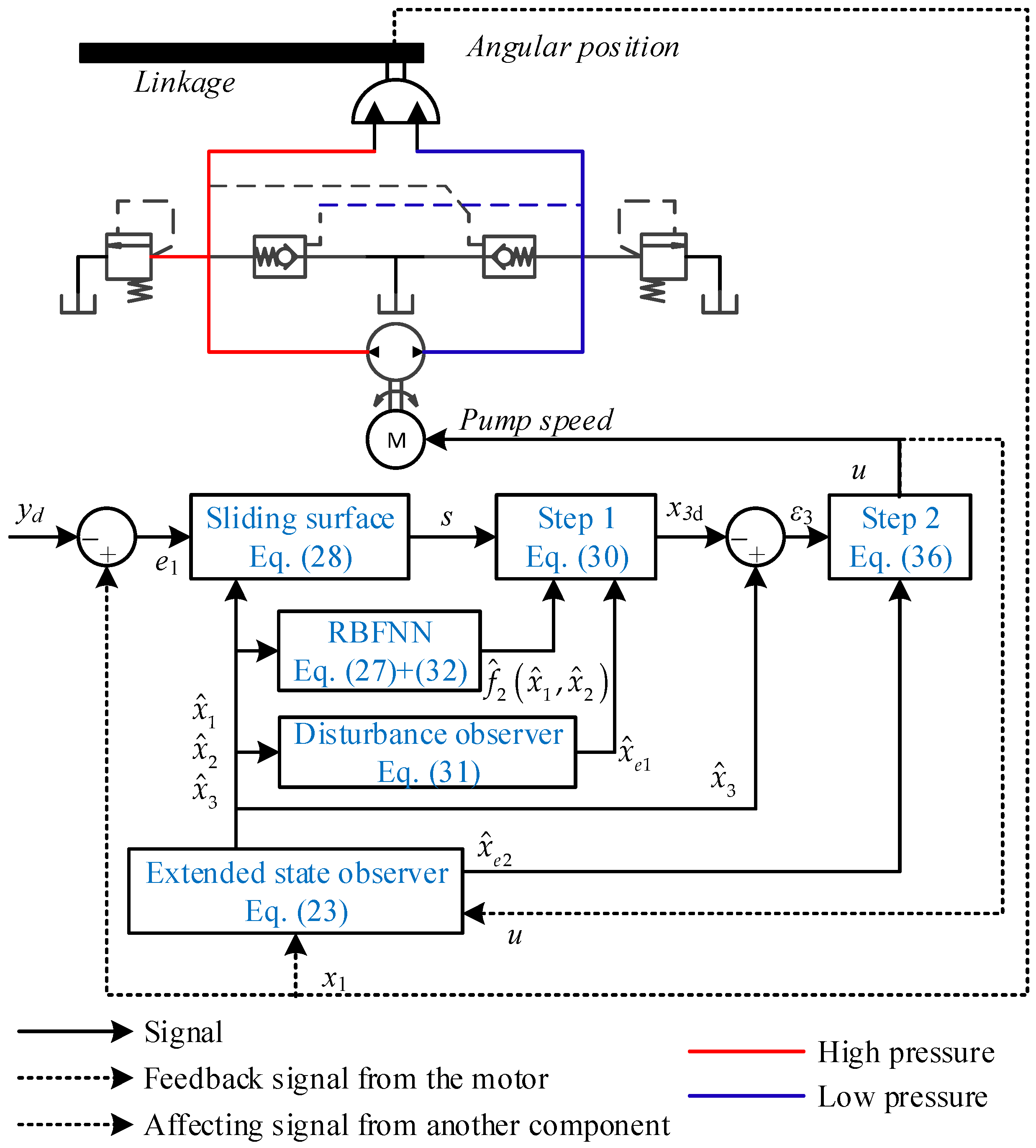
4. Estimator-Based Sliding Mode Control

The overall control architecture is sketched in Figure 2.

4.1. Control Law Implementation

Step 1: Define the tracking errors ${\epsilon }_1={\widehat{x}}_1-y_d$ and ${\epsilon }_2={\dot{\widehat{x}}}_1-{\dot{y}}_d={\widehat{x}}_2-{\dot{y}}_d={\dot{\epsilon }}_1$. A sliding mode surface s is initiated as

$$s={\dot{\epsilon }}_1+\lambda {\epsilon }_1,$$

(28)

where λ is the slope of the sliding manifold.

Based on the equivalent concept, one has s = 0 or ${\dot{\epsilon }}_1=-\lambda {\epsilon }_1$. Accordingly, the time derivative of the sliding surface s is obtained as

$$\dot{s}={\widehat{x}}_3+f_2\left({\widehat{x}}_1,{\widehat{x}}_2\right)+x_{e1}-{\ddot{y}}_d-{\lambda }^2{\epsilon }_1^2,$$

(29)

The instantaneous virtual control signal $x_{3d}$ is chosen as

$$x_{3d}={\ddot{y}}_d-{\widehat{\xi }}^T\phi \left({\widehat{\overline{x}}}_2\right)-{\widehat{x}}_{e1}+{\lambda }^2{\epsilon }_1^2-Ks,$$

(30)

where K is a positive control gain and ${\widehat{x}}_{e1}$ is an estimation of $x_{e1}$, whose dynamics are expressed based on a disturbance observer as

$$\left\{\begin{array}{l}{\widehat{x}}_{e1}=v+\omega s\\ \dot{v}=-\omega v+s-\omega \left({\widehat{\xi }}^T\phi \left({\widehat{\overline{x}}}_2\right)+{\widehat{x}}_3+\omega s\right)+\omega {\ddot{y}}_d+\omega {\lambda }^2{\epsilon }_1^2\end{array}\right.,$$

(31)

where ω > 0 is the observer gain.

The estimated weighting vector $\widehat{\xi }$ is updated through the following:

$$\dot{\hat{\xi }}=\gamma s\phi \left({\widehat{\overline{x}}}_2\right)-\zeta \widehat{\xi },$$

(32)

where γ > 0 and ζ > 0 are updating parameters.

From the above control (30), one has $0=-x_{3d}+{\ddot{y}}_d-{\widehat{x}}_{e1}+{\lambda }^2{\epsilon }_1^2-Ks$. Summing this result with (29) yields:

$$\dot{s}=\left({\widehat{x}}_3-x_{3d}\right)+{\tilde{x}}_{e1}+{\tilde{\xi }}^T\phi \left({\widehat{\overline{x}}}_2\right)+ƛ-Ks,$$

(33)

In addition, from the disturbance observer (31), by defining ${\tilde{x}}_{e1}=x_{e1}-{\widehat{x}}_{e1}$, its time derivative can be obtained:

$${\dot{\tilde{x}}}_{e1}={\dot{x}}_{e1}-\omega {\tilde{x}}_{e1}-\omega {\tilde{\xi }}^T\phi \left({\widehat{\overline{x}}}_2\right)-\omega ƛ-s,$$

(34)

Step 2: Define the tracking errors ${\epsilon }_3={\widehat{x}}_3-x_{3d}$, then $\dot{s}={\epsilon }_3+{\tilde{x}}_{e1}+{\tilde{\xi }}^T\phi \left({\widehat{\overline{x}}}_2\right)+ƛ-Ks$ is obtained. Subsequently, the time derivative of the tracking errors ${\epsilon }_3$ is:

$${\dot{\epsilon }}_3=g_3\left({\widehat{x}}_1\right)u+{\widehat{x}}_{e2}-{\dot{x}}_{3d},$$

(35)

The control signal u is derived as

$$u={\displaystyle \frac{1}{g_3\left({\widehat{x}}_1\right)}}\left({\dot{x}}_{3d}-{\widehat{x}}_{e2}-\eta {\epsilon }_3-g_{2}s\right),$$

(36)

with η > 0 being a torque control gain.

Substituting control signal u (36) into (35) brings:

$${\dot{\epsilon }}_3=-\eta {\epsilon }_3-s,$$

(37)

4.2. Closed-Loop System Stability

Theorem 2.

Given system (1), by considering the equivalent system (23), with the use of adaptive laws (31) and (32), and control laws (30) and (36), the stability of the closed-loop system is guaranteed in which all state errors are ultimately uniformly bounded and converge to the small regions of the origin.

Proof of Theorem 2.

To prove the stability of the closed-loop system, consider the following Lyapunov function W:

$$W=W_0+{\displaystyle \frac{1}{2}}{s}^2+{\displaystyle \frac{1}{2}}{\epsilon }_3^2+{\displaystyle \frac{1}{2}}{\tilde{x}}_{e1}^2+{\displaystyle \frac{1}{2\gamma }}{\tilde{\xi }}^T\tilde{\xi },$$

(38)

Taking derivative W with respect to time yields:

$$\dot{W}={\dot{W}}_0+s\dot{s}+{\epsilon }_3{\dot{\epsilon }}_3+{\displaystyle \frac{1}{\omega }}{\tilde{x}}_{e1}{\dot{\tilde{x}}}_{e1}-{\displaystyle \frac{1}{\gamma }}{\tilde{\xi }}^T\dot{\widehat{\xi }},$$

(39)

By substituting results (31)–(33) and (37), one has:

$$\begin{array}{l}\dot{W}={\dot{W}}_0+s\left(g_2{\epsilon }_3+{\tilde{x}}_{e1}+{\tilde{\xi }}^T\phi \left({\widehat{\overline{x}}}_2\right)+ƛ-Ks\right)+{\epsilon }_3\left(-\eta {\epsilon }_3-g_{2}s\right)\\ \hspace{1em}\hspace{1em}\hspace{1em}\hspace{1em}+{\tilde{x}}_{e1}\left({\dot{x}}_{e1}-\omega {\tilde{x}}_{e1}-\omega {\tilde{\xi }}^T\phi \left({\widehat{\overline{x}}}_2\right)-\omega ƛ-s\right)-{\displaystyle \frac{1}{\gamma }}{\tilde{\xi }}^T\left(\gamma {\epsilon }_3\phi \left({\widehat{\overline{x}}}_2\right)-\zeta \widehat{\xi }\right)\\ \hspace{0.17em}\hspace{0.17em}\hspace{0.17em}\hspace{0.17em}\hspace{0.17em}\hspace{0.17em}={\dot{W}}_0-K{s}^2-\eta {\epsilon }_3^2-\omega {\tilde{x}}_{e1}^2+sƛ+{\tilde{x}}_{e1}{\dot{x}}_{e1}-{\tilde{x}}_{e1}\omega {\tilde{\xi }}^T\phi \left({\widehat{\overline{x}}}_2\right)-\omega ƛ{\tilde{x}}_{e1}+{\displaystyle \frac{\zeta }{\gamma }}{\tilde{\xi }}^T\widehat{\xi },\end{array}$$

(40)

Based on Lemma 1, the following inequalities hold:

$$sƛ\le {\displaystyle \frac{{\vartheta }_1^2}{2}}{s}^2+{\displaystyle \frac{1}{2{\vartheta }_1^2}}{ƛ}^2,$$

(41)

$${\tilde{x}}_{e1}{\dot{x}}_{e1}\le {\displaystyle \frac{{\vartheta }_2^2}{2}}{\tilde{x}}_{e1}^2+{\displaystyle \frac{1}{2{\vartheta }_2^2}}{\Delta }_2^2,$$

(42)

$$-{\tilde{x}}_{e1}\omega {\tilde{\xi }}^T\phi \left({\widehat{\overline{x}}}_2\right)\le {\displaystyle \frac{{\vartheta }_3^2}{2}}\omega {\tilde{x}}_{e1}^2+{\displaystyle \frac{1}{2{\vartheta }_3^2}}\omega {\tilde{\xi }}^T\tilde{\xi }n,$$

(43)

$$-\omega ƛ{\tilde{x}}_{e1}\le {\displaystyle \frac{{\vartheta }_4^2}{2}}{\tilde{x}}_{e1}^2+{\displaystyle \frac{1}{2{\vartheta }_4^2}}{\omega }^2{ƛ}^2,$$

(44)

$${\displaystyle \frac{\zeta }{\gamma }}{\tilde{\xi }}^T\widehat{\xi }\le -{\displaystyle \frac{\zeta {\vartheta }_5^2}{2\gamma }}{\tilde{\xi }}^T\tilde{\xi }+{\displaystyle \frac{\zeta }{2\gamma {\vartheta }_5^2}}{\xi }^{*T}{\xi }^{*},$$

(45)

Subsequently, the following result is obtained:

$$\begin{array}{l}\dot{W}\le {\dot{W}}_0-\left(K-{\displaystyle \frac{{\vartheta }_1^2}{2}}\right)s^2-\eta {\epsilon }_3^2-\left(\omega -{\displaystyle \frac{{\vartheta }_2^2}{2}}-{\displaystyle \frac{\omega {\vartheta }_3^2}{2}}-{\displaystyle \frac{{\vartheta }_4^2}{2}}\right){\tilde{x}}_{e1}^2-\left({\displaystyle \frac{\zeta {\vartheta }_5^2}{2\gamma }}-{\displaystyle \frac{1}{2{\vartheta }_3^2}}\omega n\right){\tilde{\xi }}^T\tilde{\xi }\\ \hspace{0.17em}\hspace{0.17em}\hspace{0.17em}\hspace{0.17em}\hspace{0.17em}\hspace{0.17em}\hspace{0.17em}\hspace{0.17em}\hspace{0.17em}\hspace{0.17em}\hspace{0.17em}\hspace{0.17em}+{\displaystyle \frac{1}{2{\vartheta }_2^2}}{\Delta }_2^2+{\displaystyle \frac{1}{2{\vartheta }_1^2}}{ƛ}^2+{\displaystyle \frac{1}{2{\vartheta }_4^2}}{\omega }^2{ƛ}^2+{\displaystyle \frac{\zeta }{2\gamma {\vartheta }_5^2}}{\xi }^{*T}{\xi }^{*},\end{array}$$

(46)

Consequently, the time derivative $\dot{W}$ is constrained by:

$$\begin{array}{l}\dot{W}\le -{\Gamma }_0{W}_0-\left(K-{\displaystyle \frac{{\vartheta }_1^2}{2}}\right)s^2-\eta {\epsilon }_3^2-\left(\omega -{\displaystyle \frac{{\vartheta }_2^2}{2}}-{\displaystyle \frac{\omega {\vartheta }_3^2}{2}}-{\displaystyle \frac{{\vartheta }_4^2}{2}}\right){\tilde{x}}_{e1}^2-\left({\displaystyle \frac{\zeta {\vartheta }_5^2}{2\gamma }}-{\displaystyle \frac{1}{2{\vartheta }_3^2}}\omega n\right){\tilde{\xi }}^T\tilde{\xi }\\ \hspace{0.17em}\hspace{0.17em}\hspace{0.17em}\hspace{0.17em}\hspace{0.17em}\hspace{0.17em}\hspace{0.17em}\hspace{0.17em}+{\displaystyle \frac{1}{2}}{D}_2^2+{\displaystyle \frac{1}{2{\alpha }^2}}{\rho }^2+{\displaystyle \frac{1}{2{\vartheta }_2^2}}{\Delta }_2^2+{\displaystyle \frac{1}{2{\vartheta }_1^2}}{ƛ}^2+{\displaystyle \frac{1}{2{\vartheta }_4^2}}{\omega }^2{ƛ}^2+{\displaystyle \frac{\zeta }{2\gamma {\vartheta }_5^2}}{\xi }^{*T}{\xi }^{*}\\ \hspace{0.17em}\hspace{0.17em}\hspace{0.17em}\hspace{0.17em}\hspace{0.17em}\hspace{0.17em}\le -\Pi W+\Omega ,\end{array}$$

(47)

where $\Pi =\min \left\{{\Gamma }_0,2K-{\vartheta }_1^2,2\eta ,\left(2\omega -{\vartheta }_2^2-\omega {\vartheta }_3^2-{\vartheta }_4^2\right),\left(\zeta {\vartheta }_5^2-{\displaystyle \frac{\gamma }{{\vartheta }_3^2}}\omega n\right)\right\}$ and $\Omega ={\displaystyle \frac{1}{2}}{D}_2^2+{\displaystyle \frac{1}{2{\alpha }^2}}{\rho }^2+{\displaystyle \frac{1}{2{\vartheta }_2^2}}{\Delta }_2^2+{\displaystyle \frac{1}{2{\vartheta }_1^2}}{ƛ}^2+{\displaystyle \frac{1}{2{\vartheta }_4^2}}{\omega }^2{ƛ}^2+{\displaystyle \frac{\zeta }{2\gamma {\vartheta }_5^2}}{\xi }^{*T}{\xi }^{*}.$

This completed the stability proof of Theorem 2. □

Remark 2.

In view of (47), to guarantee the closed-loop system’s stability, the following conditions should be satisfied:

$$\left\{\begin{array}{l}\alpha -{\displaystyle \frac{1}{{\alpha }^2}}{\lambda }_{\max }\left(P^{T}B{B}^{T}P\right)-{\displaystyle \frac{1}{{\alpha }^2}}{\lambda }_{\max }\left(P^{T}C{C}^{T}P\right)-{\displaystyle \frac{1}{{\alpha }^4}}{\lambda }_{\max }\left(P^{T}D{D}^{T}P\right)-{\displaystyle \frac{2L_1}{\alpha }}-{\displaystyle \frac{2L_2}{{\alpha }^2}}>0\\ K-{\displaystyle \frac{{\vartheta }_1^2}{2}}>0\\ \omega -{\displaystyle \frac{{\vartheta }_2^2}{2}}-{\displaystyle \frac{\omega {\vartheta }_3^2}{2}}-{\displaystyle \frac{{\vartheta }_4^2}{2}}>0\\ {\displaystyle \frac{\zeta {\vartheta }_5^2}{2\gamma }}-{\displaystyle \frac{1}{2{\vartheta }_3^2}}\omega n>0\end{array}\right.,$$

(48)

With the inclusion of ${\vartheta }_i$ (i = 1, …, 5), the control parameters, observer gains, and updating gains can be flexibly selected for the above conditions. Conventionally, the bigger the values of gains, the faster the convergence and the better the tracking performance. However, this setting also brings a risk of the chattering phenomenon and causing instability to occur. Hence, to achieve good control performance, the control parameters and observer gains should be carefully tuned by: (1) gradually increasing the control gains K and η until the output tracking does not significantly change without chattering. Then, (2) increase the observer gain α and check the convergence of the estimated states until a small fluctuation appears. Then, α is slightly reduced to guarantee stable observability. Next, (3) gradually increase ω first and then ζ and γ and check the convergence or divergence of the approximated term ${\widehat{f}}_2(x_1,x_2)$ and ${\widehat{x}}_{e1}$. Finally, (4), the values of tuned control parameters and observer gains can all be slightly decreased to guarantee stability and reduce the risk of chattering occurrence.

5. Numerical Simulation

5.1. Examined Scenario

In this section, numerical comparative simulations are initialized using Matlab/Simulink (R2024a) environment with the sampling time of 0.1 [ms], to demonstrate the effectiveness of the proposed output feedback-based control algorithm. For this purpose, three other control strategies are involved: a model-free proportional–integral–derivative (PID) control (C1), the ESO-based robust output feedback control [27] (C2), and the output feedback with dual-ESO [31] (C3). The proposed control scheme is designated as C4. It is noted that due to the unknown friction and disturbance, the control law expressions of C2 and C3 are modified.

The PID control (C1) is a model-free method, which only treats an output $x_1$ to derive the control signal u.

The ESO-based output feedback control (C2) is considered since its control architecture is similar to the proposed method; however, the authors did not take the mismatched disturbance into consideration. Thus, the inclusion of (C2) is to demonstrate the importance of suppressing the mismatched disturbance in improving the output tracking performance. The control implementations of (C4) are derived as

$$x_{3d}^{C3}={\displaystyle \frac{1}{g_2}}\left({\ddot{y}}_d+{\lambda }^2{\epsilon }_1^2-Ks\right)$$

(49)

$$u_{C2}={\displaystyle \frac{1}{g_3\left(x_1\right)}}\left({\dot{x}}_{3d}^{C3}-{\widehat{x}}_{e2}-\eta {\epsilon }_3-g_{2}s\right),$$

(50)

The dual-ESO-based control (C3) took care of the mismatched disturbance; nevertheless, the realization of including this parameter in the control law implementation and its effectiveness have not been evaluated. Additionally, the authors investigated the case with well-known nominal friction. Therefore, in this comparison, the assumed well-known friction in C3 is relaxed, and thus C3 is involved to clarify the importance of tackling this nonlinear term. The control modification of (C3) is as follows:

$$x_{3d}^{C3}={\displaystyle \frac{1}{g_2}}\left({\ddot{y}}_d-{\widehat{x}}_{e1}+{\lambda }^2{\epsilon }_1^2-Ks\right)$$

(51)

$$u_{C3}={\displaystyle \frac{1}{g_3\left(x_1\right)}}\left({\dot{x}}_{3d}^{C3}-{\widehat{x}}_{e2}-\eta {\epsilon }_3-g_{2}s\right),$$

(52)

The goal is to regulate the system output to follow the desired trajectory: $y_d={\displaystyle \raisebox{1ex}{$30\pi $}\!\left/ \!\raisebox{-1ex}{$180$}\right.}\sin \left({\displaystyle \raisebox{1ex}{$2\pi t$}\!\left/ \!\raisebox{-1ex}{$T$}\right.}\right)$ (rad) where T is the period (s) under the friction $f_2=b_1{x}_2+b_2\mathrm{t}\mathrm{a}\mathrm{n}\mathrm{h}\left({10}^4{x}_2\right)$ and time-varying external disturbance ${\tau }_{ext}$, including the external load ${\tau }_{load}$ and influence of the gravity effect on the linkage (assumed to be absolutely stiff with equally distributed mass). Accordingly, the disturbance is shown by:

$${\delta }_2=-\left[{\tau }_{load}+{\displaystyle \frac{1}{2J}}MgL\sin \left(x_1\right)\right] \left(\mathrm{Nm}\right),$$

(53)

where M is the total linkage mass, g = 9.81 m²/s is the gravity acceleration, and L is the linkage length.

The system parameters of the EHPS, with hydraulic and mechanical parts, are described in

Table 1. EHPS parameters—hydraulic part [31].

Parameter (Unit)	Symbol	Value	(SI Unit)
Bulk modulus	β	1.5 × 109	N/m2
Pump displacement	Dp	0.1544 × 10–7	m3/rad
Pump coefficient	KPump	10	rad/s/vol
Initial volume of chamber 1	V01	7.368 × 10–6	m3
Initial volume of chamber 2	V02	7.368 × 10–6	m3
Gradient cross-section area	A	5.8422 × 10–6	m3/rad
Leakage coefficient	Ct	4.267 × 10–12

and

Table 2. EHPS parameters—mechanical part [31].

Parameter (Unit)	Symbol	Value	(SI Unit)
Actuator moment inertia	J	0.2	kg/m2
Viscous friction coefficient		10	Nms/rad
Coulomb friction coefficient		10	Nm
Linkage mass	M	0.1	kg
Linkage length	L	0.5	m
External load	${\tau }_{load}$	20	Nm

and the controller gains are selected as shown in

Table 3. Control parameters.

Controllers	Control Parameters
C1	$k_P=1000,\hspace{0.17em}{k}_I=1000,\hspace{0.17em}{k}_D=0.01$
C2	$K=300,\hspace{0.17em}\eta =1500,\hspace{0.17em}\lambda =2$ Observer: Matched uncertainty estimation: α = 800 (ESO).
C3	$K=300,\hspace{0.17em}\eta =1500,\hspace{0.17em}\lambda =2$ Observers: Matched uncertainty estimation: α = 800 (ESO-1); mismatched disturbance estimation: ω = 800 (ESO-2).
C4	$K=300,\hspace{0.17em}\eta =1500,\hspace{0.17em}\lambda =2$ The estimators are structured as follows: $\mathrm{RBFNN}: m={\left[m_1,\hspace{0.17em}\hspace{0.17em}{m}_2,\hspace{0.17em}\hspace{0.17em}{m}_3,\hspace{0.17em}\hspace{0.17em}{m}_4,\hspace{0.17em}\hspace{0.17em}{m}_5\right]}^T$$\mathrm{with} m_1={\displaystyle \frac{1}{10}}{A}_0\omega \left[-10,-9,-8,-7,\right.-6,$${\left.-5,-4,-3,-2,-1,0,1,2,3,4,5,6,7,8,9,10\right]}^T$$, m_k={\displaystyle \frac{1}{10}}\left[-10,-9,-8,-7,\right.-6,-5,$ ${\left.-4,-3,-2,-1,0,1,2,3,4,5,6,7,8,9,10\right]}^T$$(k=2, 3, 4, 5); {\sigma }_i=2 (i=1, \dots , 5), \gamma =1.25 \times {10}^4; \mathsf{\zeta }={10}^{-1}, \mathrm{initial} \mathrm{weighting} \mathrm{vector}: \widehat{\xi }(0)=0.1\times \mathrm{ones}\left(21,1\right)$ with ones(21,1) being the column unit vector of 21 rows. Observers: Matched uncertainty estimation: α = 800 (ESO); mismatched disturbance estimation: ω = 50 (DO).

.

Remark 3.

In light of [33,34], the control signal u under C2, C3, and C4 (or the backstepping control framework in general) follows the form of an adaptive PID control with time-varying adaptive equivalent $k_{P,eq}$, $k_{I,eq}$, and $k_{D,eq}$ gains regarding tracking errors and adaptive laws presented above, i.e., $u=k_{P,eq}{\epsilon }_1+k_{I,eq}{\displaystyle \underset{0}{\overset{t}{\int }}{\epsilon }_{1}d\tau }+k_{D,eq}{\dot{\epsilon }}_1+f_{fract}+f_{dyn}$ with $f_{fract}$ being the fractional order term and $f_{dyn}$ being the dynamical terms. Moreover, $k_{P,eq}$, $k_{I,eq}$, and $k_{D,eq}$ also include the approximated dynamics. Hence, for a fair comparison, the controller gains of C1 (PID gains) should be selected such that they are greater than the corresponding equivalent gains, i.e., $k_{P,C1}\ge max\left(k_{P,eq}\right)$, $k_{I,C1}\ge max\left(k_{I,eq}\right)$, and $k_{D,C1}\ge max\left(k_{D,eq}\right)$ without chattering phenomenon incurrence.

To better demonstrate the effectiveness of the proposed methodology, the setup simulation is composed of three scenarios:

• Scenario 1: No leakage and no disturbance, from the beginning to 6 s.
• Scenario 2: No disturbance and the leakage suddenly occurs at t = 6 s.
• Scenario 3: The load torque ${\tau }_{load}$ suddenly occurs at t = 12 s along with the leakage.

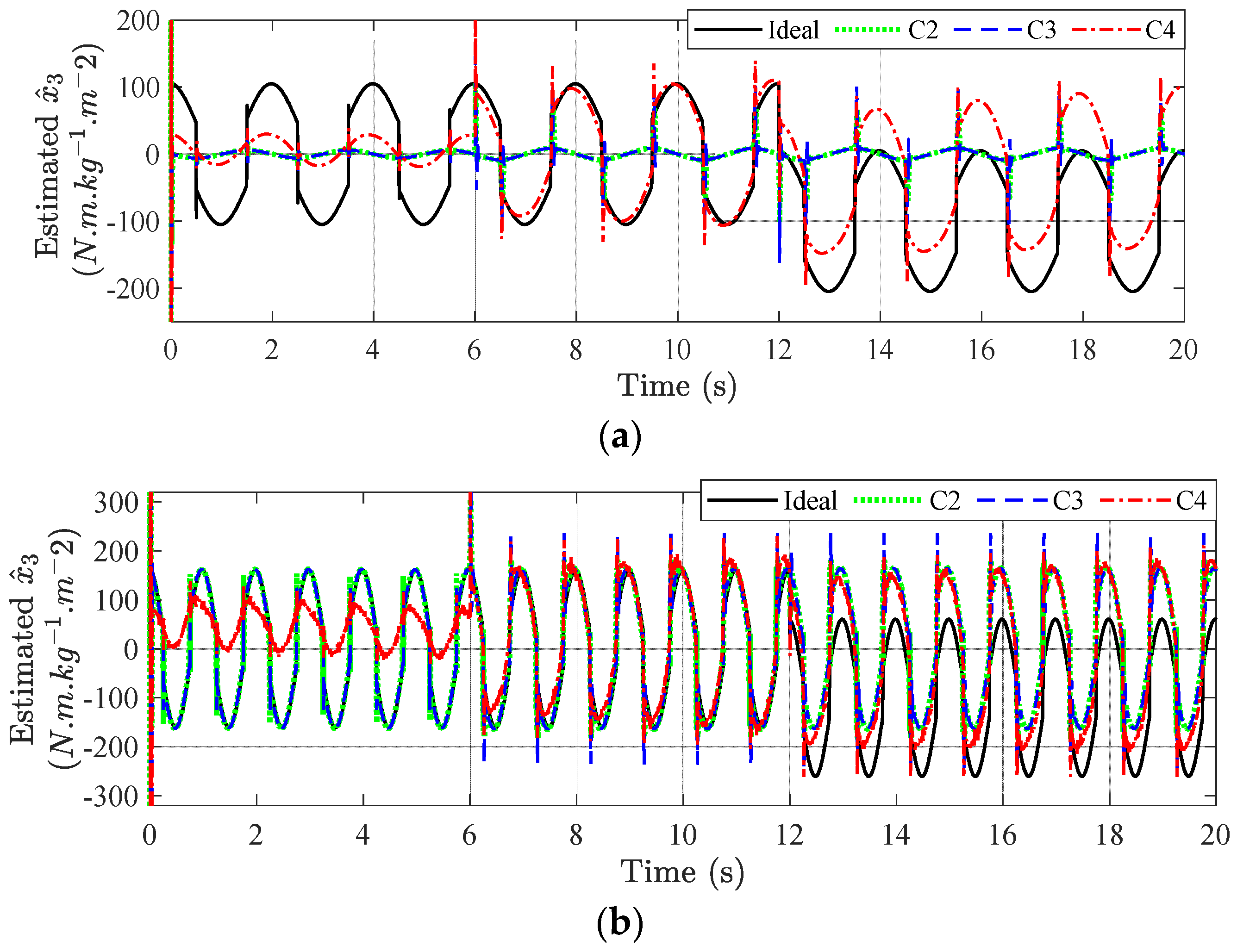
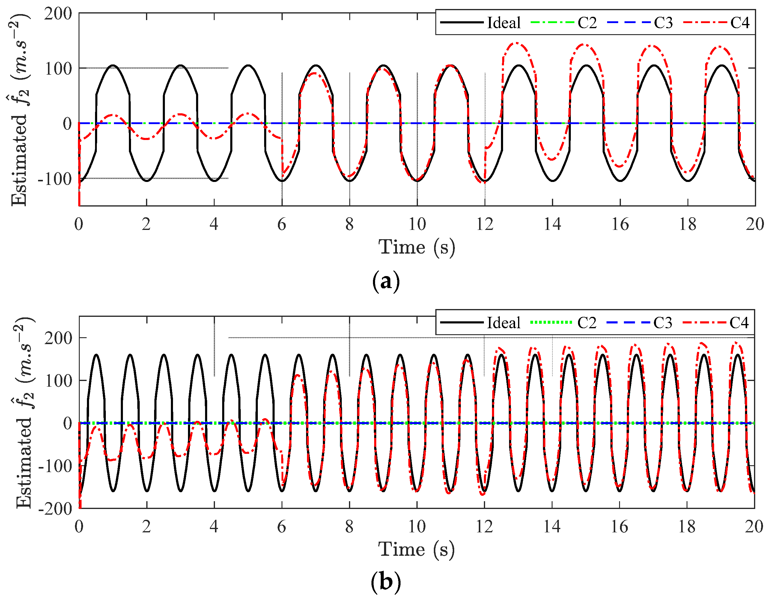
In this paper, the sampling time is set as $t_s={10}^{-4}\left(s\right)$ and the simulation time is t_period = 20 (s). Additionally, bandwidth-limited white noise is also added to the measured output to emulate the measurement noise in practice. Accordingly, a low-pass filter, with the cut-off frequency of $f_{cut}=1/t_s$ (Hz), is added to suppress this impact.

5.2. Main Results

The angular output tracking efforts are shown in Figure 3, while Figure 4 reveals the angular velocity qualification, with low-frequency movement (a) and high-frequency movement (b). In each graph, the upper sub-figures show tracking performance and the bottom sub-figures show tracking errors.

As seen, the model-free PID performed the worst tracking regulation due to not considering the system behaviors and suppressing uncertainties. Moreover, under the occurrence of internal leakage and external load impact, it could not satisfy the desired trajectory. Without leakage and external payload, the output tracking errors were in the ranges of ±2.4 (degree) in low-frequency movement and ±4.65 (degree) in high-frequency movement while the angular velocity tracking error, in the steady state, was in the ranges of ±12.2 (degree/s) at low-frequency and ±38.5 (degree/s) at high-frequency movements, as shown in Figure 3. Even when increasing controller gains, it could not guarantee robustness against the impacts of leakage and payload in which its output tracking errors expanded up to ±12 (degree) at low-frequency and ±15 (degree) at high-frequency movements. The angular velocity tracking errors were in the ranges of ±45.3 (degree/s) at low-frequency and nearly ±100 (degree/s) at high-frequency trajectories, as displayed in Figure 4.

On the contrary, the other three control strategies, C2, C3, and the proposed C4, could accomplish output tracking satisfaction and robustness against the adverse influence of uncertainties.

In detail, the comparative method C2 could satisfy the output tracking demand in three situations. With the matched uncertainty estimated and hydraulic actuator dynamics consideration $g_3(x_1)$, the output performance was significantly improved with the small output tracking errors, in the range of ±0.36 (degree) at low-frequency and ±0.6 (degree) at high-frequency movements, with the velocity error being in the ranges of ±5.5 (degree/s) at low-frequency and ±10.2 (degree/s) at high-frequency movements in the steady state. Moreover, with the ESO employed, the behavior of lumped matched uncertainty ${\widehat{x}}_{e2}={\widehat{f}}_3(x_1,x_2,x_3)$ could be well estimated in comparison with the ideal ${x_{e2}=f}_3(x_1,x_2,x_3)$ as indicated in Figure 5. It is worth noting that the ideal dynamics $f_3(x_1,x_2,x_3)$ was obtained based on applying the ideal model-based BSC where all system parameters were well defined. However, due to ignoring the influences of mismatched disturbance and unknown friction $f_2\left({\overline{\mathbf{x}}}_2\right)$, the control performance was extensively affected similar to the maximum transient output tracking error mentioned above.

With the mismatched disturbance pointed out, C3 could improve the output tracking qualification compared to C2. The output tracking errors were reduced to ±0.16 (degree) and ±0.26 (degree) at low- and high-frequency movements, respectively. The ranges of the velocity tracking errors were approximately ±6 (degree/s) in the steady state as shown in Figure 2 and Figure 3, respectively. When the same ESO mechanism is employed, the lumped systematic uncertainty ${\widehat{f}}_3(x_1,x_2,x_3)$ could be well estimated, the same as the one under C2. However, the overshoot when leakage and load disturbance occurred was significantly reduced owing to the development of the dual-ESO to address the load disturbance in the control expression (50). Nonetheless, similar to C2, the estimated active torque ${\widehat{x}}_3$ could follow the actual $x_3$ as indicated in Figure 6.

As observed in Figure 6 with both situations, due to only using the output $x_1$ and its estimated ${\widehat{x}}_1$ for the lumped matched uncertainty and variable $x_3$ estimations, the estimated ${\widehat{x}}_3$ was a result of the estimated error $x_1-{\widehat{x}}_1$. Thereby, the estimated ${\widehat{x}}_3$ could not correctly reflect the behavior of real $x_3$, which was only affected by the external load torque ${\tau }_{ext}$ forcing on the mechanical part. Herein, the benchmark active torque was obtained by applying the model-based BSC to the system with the same control parameters and working conditions. Even when utilizing C3 with the dual-ESO, the active torque and mismatched disturbance $x_{e1}$ could not be well estimated due to the influence of unknown friction $f_2\left({\overline{\mathbf{x}}}_2\right)$, as disclosed in Figure 7. Both estimated ${\widehat{x}}_3$ under C2 and C3 varied around zero as a result of being estimated via the term $x_1-{\widehat{x}}_1$.

Meanwhile, the proposed C4 could not only exhibit the best tracking qualification in the tracking regulations and lumped matched dynamics estimation but also achieve acceptable estimated active torque ${\widehat{x}}_3$. As seen in Figure 3, C4 performed the smallest output tracking error with the least overshoot in the transient state compared to C3. The overshoots of the output tracking efforts were remarkably reduced, of which the maximum overshoots were only ±0.14 (degree) at low-frequency and ±0.25 (degree) at high-frequency movements for the output tracking error. Of the velocity tracking qualification, the tracking errors were distributed in the intervals of ±1.35 (degree/s) at low-frequency and ±2.6 (degree/s) at high-frequency movements.

The lumped matched dynamical behavior ${\widehat{f}}_3(x_1,x_2,x_3)$ was well estimated as the consequence of using the same structured ESO. Moreover, the estimated active torque ${\widehat{x}}_3$ could be partly reflected compared to the real one and the unknown friction could also be observed in part as demonstrated in Figure 7. Unfortunately, the external disturbance load could not be well estimated regardless of control strategy as shown in Figure 8. The reason is the coupled influence between the state-dependent friction $f_2\left({\overline{\mathbf{x}}}_2\right)$ and partly state-dependent external disturbance ${\delta }_2$ as presented in (52). Moreover, regarding the DO mechanism (31), ${x_{e1}=\delta }_2$ was structured as the function of sliding surface s, tracking error ${\epsilon }_1$, estimated ${\widehat{x}}_3$, and estimated dynamical term ${\widehat{f}}_2\left({\overline{\mathbf{x}}}_2\right)$. Thus, if ${\widehat{x}}_3$ could not well reflect the actual $x_3$ and ${\widehat{f}}_2\left({\widehat{\overline{\mathbf{x}}}}_2\right)$ could not be well approximated, ${\delta }_2$ could not be obtained and a part of ${\delta }_2$ certainly lumped into ${\widehat{f}}_2\left({\overline{\mathbf{x}}}_2\right)$. Similarly, in the case of C3 with dual-ESO, $x_{e1}$ was structured as a function of estimated error between the estimated ${\widehat{x}}_3$ and its second-time estimation when employing the dual-ESO. As ${\widehat{x}}_3$ was incorrectly observable compared to the real $x_3$, its second-time estimation could not converge to $x_3$ but only follow ${\widehat{x}}_3$. Additionally, with the $f_2\left({\overline{\mathbf{x}}}_2\right)$ being ungoverned, it was impossible to reconstruct $x_{e1}$ as a result.

The control signals under the four methodologies are depicted in Figure 9. Generally, there was no chattering phenomenon, which suggests the possibility of realizing a real prototype. In consequence, the superiority of the proposed C4 over the other algorithms is summarized via several performance indexes as shown in

Table 4. Performance indexes under low-frequency movement.

Controller	$\sqrt{\frac{1}{{\mathit{N}}_{\Delta \mathit{t}}}{\displaystyle \sum _{\mathit{k}=1}^{{\mathit{N}}_{\Delta \mathit{t}}}{\mathit{\epsilon }}_{1,\mathit{k}}^2}}$ (Degree)	$\mathbf{Max} \mathbf{Transient} \left|{\mathit{\epsilon }}_1\right|$ in Steady State (Degree)	$\mathbf{Max} \mathbf{Transient} \left|{\mathit{\epsilon }}_2\right|$ in Steady State (Degree/s)	Scenario
C1	17.3649	2.368	12.147	1
		8.048	45.35	2
		12.07	45.281	3
C2	1.3371	0.053	1.243	1
		0.355	5.443	2
		0.3623	5.5	3
C3	0.8178	0.0263	1.96	1
		0.1607	5.433	2
		0.1608	5.482	3
C4	0.4525	0.0225	0.367	1
		0.1371	1.289	2
		0.1371	1.324	3

for low frequency and in

Table 5. Performance indexes under high-frequency movement.

Controller	$\sqrt{\frac{1}{{\mathit{N}}_{\Delta \mathit{t}}}{\displaystyle \sum _{\mathit{k}=1}^{{\mathit{N}}_{\Delta \mathit{t}}}{\mathit{\epsilon }}_{1,\mathit{k}}^2}}$ (Degree)	$\mathbf{Max} \mathbf{Transient} \left|{\mathit{\epsilon }}_1\right|$ in Steady State (Degree)	$\mathbf{Max} \mathbf{Transient} \left|{\mathit{\epsilon }}_2\right|$ in Steady State (deg/s)	Scenario
C1	48.2949	4.6491	38.4626	1
		12.2459	98.5342	2
		15.1787	98.895	3
C2	3.0044	0.1436	1.2942	1
		0.598	9.8975	2
		0.6097	10.1341	3
C3	1.9664	0.0576	1.771	1
		0.2557	5.6202	2
		0.2644	6.1146	3
C4	1.1271	0.0574	0.8703	1
		0.2178	1.9366	2
		0.2237	2.5589	3

for high frequency with logarithmic scaling graphs of root mean square errors in Figure 10.

Additionally, it should be noted that according to the original works [27,31], the authors considered the well-known structured friction $f_2\left({\overline{\mathbf{x}}}_2\right)$ and thus its estimated $f_2\left({\widehat{x}}_2\right)=b_1{\widehat{x}}_2+b_2\mathrm{s}\mathrm{i}\mathrm{g}\mathrm{n}\left({\widehat{x}}_2\right)$ with well-defined $b_1$ and $b_2$ was utilized. However, in our examined case studies, we considered the poorly known structured friction, i.e., the structured dynamical term $f_2\left({\overline{\mathbf{x}}}_2\right)$ is completely unknown for fair comparisons. Fortunately, the integration of the RBFNN and DO helped overcome this obstacle as the results demonstrate in Figure 3 and Figure 4. Therefore, this difficulty motivates us to find an effective solution to reconstruct the external impact $x_{e1}$ and dynamics $f_2\left({\overline{\mathbf{x}}}_2\right)$ in the future.

6. Conclusions

This paper proposed the output feedback-based robust BSMC for uncertain EHPSs, subject to unknown disturbance, uncertainties, and unstructured dynamical models. To deal with these issues, the ESO was first established to deal with the lumped mismatched uncertainty. For the problem of unstructured dynamics of the mechanical part, the RBFNN-based approximation mechanism was then employed to compensate for its influence. Additionally, unknown external disturbance was also eliminated in this manner using disturbance observer-based adaptive law. With all unstructured dynamical terms estimated, the robust BSMC was then derived to manipulate the system output to follow the desired trajectory. Generally, under the proposed control algorithm, unknown disturbance, uncertainty, and unstructured dynamical terms could be estimated in which their estimation could match the ideal ones, under the model-based BSMC. As a result, the output tracking performance could be improved in which its tracking qualification was nearly the same as that of the model-based benchmark. Future works will clarify the influence of pump dynamics and improve the control performance with constraints. In addition, the influence of measurement noise on the system at high-frequency movement will also be detailed to strengthen the control robustness.

References

1. Shang, Y.; Li, X.; Qian, H.; Wu, S.; Pan, Q.; Huang, L.; Jiao, Z. A Novel Hydrostatic Actuator System with Energy Recovery Module for More Electric Aircraft. IEEE Trans. Ind. Electron. 2020, 67, 2991–2999. [Google Scholar] [CrossRef]
2. Du, S.; Zhou, J.; Zhao, H.P.; Ma, S. Research on the energy transfer and efficiency performance of an electro-hydrostatic actuator for wheel-legged robot joint. Energy 2024, 291, 130417. [Google Scholar] [CrossRef]
3. Staman, K.; Veale, A.J.; Kooij, A. Design, Control and Evaluation of the Electro-Hydrostatic Actuator, PREHydrA, for Gait Restoration Exoskeleton Technology. IEEE Trans. Med. Robot. Bionics 2021, 3, 156–165. [Google Scholar] [CrossRef]
4. Sun, M.; Ouyang, X.; Mattila, J.; Chen, Z.; Yang, H.; Liu, H. Lightweight Electrohydrostatic Actuator Drive Solution for Exoskeleton Robots. IEEE/ASME Trans. Mechatron. 2022, 27, 4631–4642. [Google Scholar] [CrossRef]
5. Lee, W.; Kim, M.J.; Chung, W.K. Asymptotically stable disturbance observer-based compliance control of electrohydrostatic actuators. IEEE/ASME Trans. Mechatron. 2020, 25, 195–206. [Google Scholar] [CrossRef]
6. Feng, H.; Yin, C.; Cao, D. Trajectory Tracking of an Electro-Hydraulic Servo System with an New Friction Model-Based Compensation. IEEE/ASME Trans. Mechatron. 2023, 28, 473–482. [Google Scholar] [CrossRef]
7. Wang, Q.; Du, Z.; Chen, W.; Ai, C.; Kong, X.; Zhang, J.; Liu, K.; Chen, G. Maximum Power Point Tracking Control of Offshore Hydraulic Wind Turbine Based on Radial Basis Function Neural Network. Energies 2024, 17, 449. [Google Scholar] [CrossRef]
8. Kumar, D.; Mahato, A.C. An accumulator-based hydro-mechanical power transmission technology for smoothing the power output from a wind turbine. Sādhanā 2023, 48, 241. [Google Scholar] [CrossRef]
9. Nie, Y.; Lao, Z.; Liu, J.; Huang, Y.; Sun, X.; Tang, J.; Chen, Z. Disturbance Observer-Based Sliding Mode Controller for Underwater Electro-Hydrostatic Actuator Affected by Seawater Pressure. Machines 2022, 10, 1115. [Google Scholar] [CrossRef]
10. Ahn, K.K.; Nam, D.N.C.; Jin, M.L. Adaptive Backstepping Control of an Electrohydraulic Actuator. IEEE/ASME Trans. Mechatron. 2014, 19, 987–995. [Google Scholar] [CrossRef]
11. Huang, L.; Yu, T.; Jiao, Z.; Li, Y. Research on Power Matching and Energy Optimal Control of Active Load-Sensitive Electro-Hydrostatic Actuator. IEEE Access 2021, 9, 51121–51133. [Google Scholar] [CrossRef]
12. Liu, J.; Hu, Y.; Zhu, Z.; Zhao, Z.; Gao, G.; Yao, J. Intelligent fault diagnosis for electro-hydrostatic actuator based on multisource information convolutional residual network. Meas. Sci. Technol. 2024, 35, 066114. [Google Scholar] [CrossRef]
13. Liu, J.; Huang, Y.; Helian, B.; Nie, Y.; Chen, Z. Flow match and precision motion control of asymmetric electro-hydrostatic actuators with complex external force in four-quadrants. J. Frankl. Inst. 2024, 36, 1025–1039. [Google Scholar] [CrossRef]
14. Truong, D.Q.; Ahn, K.K. Force control for hydraulic load simulator using self-tuning grey predictor—Fuzzy PID. Mechatronics 2009, 19, 233–246. [Google Scholar] [CrossRef]
15. Wang, H.; Zhang, Y.; Li, G.; Liu, R.; Zhou, X. Design and Control of an Energy-Efficient Speed Regulating Method for Pump-Controlled Motor System under Negative Loads. Machines 2023, 11, 437. [Google Scholar] [CrossRef]
16. Ma, W.; Ma, S.; Qiao, W.; Cao, D.; Yin, C. Research on PID Controller of Excavator Electro-Hydraulic System Based on Improved Differential Evolution. Machines 2023, 11, 143. [Google Scholar] [CrossRef]
17. Cao, F. PID controller optimized by genetic algorithm for direct-drive servo system. Neural Comput. Appl. 2020, 32, 23–30. [Google Scholar] [CrossRef]
18. To, X.D.; Tran, D.T.; Truong, H.V.A.; Ahn, K.K. Disturbance Observer Based Finite Time Trajectory Tracking Control for a 3 DOF Hydraulic Manipulator Including Actuator Dynamics. IEEE Access 2018, 6, 36798–36809. [Google Scholar]
19. Chen, Y.; Zhang, Q.; Tian, Q.; Feng, X. Extended State Observer-Based Fuzzy Adaptive Backstepping Force Control of a Deep-Sea Hydraulic Manipulator with Long Transmission Pipelines. J. Mar. Sci. Eng. 2022, 10, 1467. [Google Scholar] [CrossRef]
20. Mi, J.; Deng, W.; Yao, J.; Liang, X. Linear-Extended-State-Observer-Based Adaptive RISE Control for the Wrist Joints of Manipulators with Electro-Hydraulic Servo Systems. Electronics 2024, 13, 1060. [Google Scholar] [CrossRef]
21. Dao, H.V.; Na, S.; Nguyen, D.G.; Ahn, K.K. High accuracy contouring control of an excavator for surface flattening tasks based on extended state observer and task coordinate frame approach. Autom. Constr. 2021, 130, 103845. [Google Scholar] [CrossRef]
22. Ba, D.X.; Dinh, Q.T.; Bae, J.; Ahn, K.K. An Effective Disturbance-Observer-Based Nonlinear Controller for a Pump-Controlled Hydraulic System. IEEE/ASME Trans. Mechatron. 2020, 25, 32–43. [Google Scholar] [CrossRef]
23. Trinh, H.A.; Truong, H.V.A.; Ahn, K.K. Fault Estimation and Fault-Tolerant Control for the Pump-Controlled Electrohydraulic System. Actuators 2020, 9, 132. [Google Scholar] [CrossRef]
24. Zhang, S.; Li, S.; Dai, F. Integral Sliding Mode Backstepping Control of an Asymmetric Electro-Hydrostatic Actuator Based on Extended State Observer. Proceedings 2020, 64, 13. [Google Scholar] [CrossRef]
25. Shen, W.; Zhao, H. Fault tolerant control of nonlinear hydraulic systems with prescribed performance constraint. ISA Trans. 2022, 131, 1–14. [Google Scholar] [CrossRef] [PubMed]
26. Lao, L.; Chen, P. Adaptive Sliding Mode Control of an Electro-Hydraulic Actuator with a Kalman Extended State Observer. IEEE Access 2024, 12, 8970–8982. [Google Scholar] [CrossRef]
27. Yao, J.; Jiao, Z.; Ma, D. Extended-State-Observer-Based Output Feedback Nonlinear Robust Control of Hydraulic Systems with Backstepping. IEEE Trans. Ind. Electron. 2014, 61, 6285–6293. [Google Scholar] [CrossRef]
28. Yang, G.; Yao, J. Output feedback control of electro-hydraulic servo actuators with matched and mismatched disturbances rejection. J. Frankl. Inst. 2019, 356, 9152–9179. [Google Scholar] [CrossRef]
29. Yang, X.; Yao, J.; Deng, W. Output feedback adaptive super-twisting sliding mode control of hydraulic systems with disturbance compensation. ISA Trans. 2021, 109, 175–185. [Google Scholar] [CrossRef]
30. Tran, D.T.; Do, T.C.; Ahn, K.K. Extended High Gain Observer-Based Sliding Mode Control for an Electro-hydraulic System with a Variant Payload. Int. J. Precis. Eng. Manuf. 2019, 20, 2089–2100. [Google Scholar] [CrossRef]
31. Nguyen, M.H.; Ahn, K.K. Output Feedback Robust Tracking Control for a Variable-Speed Pump-Controlled Hydraulic System Subject to Mismatched Uncertainties. Mathematics 2023, 11, 1783. [Google Scholar] [CrossRef]
32. Ye, N.; Song, J.; Ren, G. Model-Based Adaptive Command Filtering Control of an Electrohydraulic Actuator with Input Saturation and Friction. IEEE Access 2020, 8, 48252–48263. [Google Scholar] [CrossRef]
33. Truong, H.V.A.; Nam, S.; Kim, S.; Kim, Y.; Chung, W.K. Backstepping-Sliding-Mode-Based Neural Network Control for Electro-Hydraulic Actuator Subject to Completely Unknown System Dynamics. IEEE Trans. Autom. Sci. Eng. 2023. Early access. [Google Scholar] [CrossRef]
34. Truong, H.V.A.; Nguyen, M.H.; Tran, D.T.; Ahn, K.K. A novel adaptive neural network-based time-delayed estimation control for nonlinear systems subject to disturbances and unknown dynamics. ISA Trans. 2023, 142, 214–227. [Google Scholar] [CrossRef] [PubMed]
35. Truong, H.V.A.; Phan, V.D.; Tran, D.T.; Ahn, K.K. A novel observer-based neural-network finite-time output control for high-order uncertain nonlinear systems. Appl. Math. Comput. 2024, 475, 128699. [Google Scholar] [CrossRef]
36. Phan, V.D.; Vo, C.P.; Dao, H.V.; Ahn, K.K. Robust Fault-Tolerant Control of an Electro-Hydraulic Actuator with a Novel Nonlinear Unknown Input Observer. IEEE Access 2021, 9, 30750–30760. [Google Scholar] [CrossRef]
37. Han, S.; Wang, H.; Tian, Y.; Christov, N. Time-delay estimation based computed orque control with robust adaptive RBF neural network compensator for a rehabilitation exoskeleton. ISA Trans. 2020, 97, 171–181. [Google Scholar] [CrossRef]
38. Deng, W.; Yao, J. Extended-State-Observer-Based Adaptive Control of Electrohydraulic Servomechanisms without Velocity Measurement. IEEE/ASME Trans. Mechatron. 2020, 25, 1151–1161. [Google Scholar] [CrossRef]
39. Yao, J.; Jiao, Z.; Ma, D.; Yan, L. High-Accuracy Tracking Control of Hydraulic Rotary Actuators with Modeling Uncertainties. IEEE/ASME Trans. Mechatron. 2014, 19, 633–641. [Google Scholar] [CrossRef]
Figure 1. A simple schematic of an EHPS.
Machines 12 00554 g001
Figure 2. Proposed output feedback control architecture.
Machines 12 00554 g002
Figure 3. Output tracking qualification under four control strategies in low-frequency movement (a) and high-frequency movement (b). (Top) Output tracking performance, (Bottom) Output tracking errors ( ε 1 ) with their zoomed-in views.
Machines 12 00554 g003
Figure 4. Velocity tracking qualification under four control strategies in low-frequency movement (a) and high-frequency movement (b). (Top) Velocity tracking performance, (Bottom) velocity tracking errors ( ε 2 ) with their zoomed-in views.
Machines 12 00554 g004
Figure 5. The estimations of x ^ e 2 = f ^ 3 ( x 1 , x 2 , x 3 ) under C2, C3, and C4 compared to the ideal model-based BSC with low-frequency movement (a) and high-frequency movement (b).
Machines 12 00554 g005
Figure 6. The estimations of x ^ 3 under C2, C3, and C4 compared to the ideal model-based BSC x3 under low-frequency movement (a) and high-frequency movement (b).
Machines 12 00554 g006
Figure 7. The estimations of f ^ 2 ( x ¯ 2 ) under C2, C3, and C4 compared to the ideal model-based BSC under low-frequency movement (a) and high-frequency movement (b).
Machines 12 00554 g007
Figure 8. The estimations of δ ^ 2 under C2, C3, and C4 compared to the ideal model-based BSC under low-frequency movement (a) and high-frequency movement (b).
Machines 12 00554 g008
Figure 9. Control signal u under four control strategies under low-frequency movement (a) and high-frequency movement (b).
Machines 12 00554 g009
Figure 10. Logarithmic scaling graphs of RMSE under two case studies: (a) low-frequency movement and (b) high-frequency movement.
Machines 12 00554 g010