Abstract
This research article proposes a new method for an enhanced Flexible Manufacturing System (FMS) using a combination of smart methods. These methods use a set of three technologies of Industry 4.0, namely Artificial Intelligence (AI), Digital Twin (DT), and Wi-Fi-based indoor localization. The combination tackles the problem of asset tracking through Wi-Fi localization using machine-learning algorithms. The methodology utilizes the extensive “UJIIndoorLoc” dataset which consists of data from multiple floors and over 520 Wi-Fi access points. To achieve ultimate efficiency, the current study experimented with a range of machine-learning algorithms. The algorithms include Support Vector Machines (SVM), Random Forests (RF), Decision Trees, K-Nearest Neighbors (KNN) and Convolutional Neural Networks (CNN). To further optimize, we also used three optimizers: ADAM, SDG, and RMSPROP. Among the lot, the KNN model showed superior performance in localization accuracy. It achieved a mean coordinate error (MCE) between 1.2 and 2.8 m and a 100% building rate. Furthermore, the CNN combined with the ADAM optimizer produced the best results, with a mean squared error of 0.83. The framework also utilized a deep reinforcement learning algorithm. This enables an Automated Guided Vehicle (AGV) to successfully navigate and avoid both static and mobile obstacles in a controlled laboratory setting. A cost-efficient, adaptive, and resilient solution for real-time tracking of assets is achieved through the proposed framework. The combination of Wi-Fi fingerprinting, deep learning for localization, and Digital Twin technology allows for remote monitoring, management, and optimization of manufacturing operations.
1. Introduction
The latest ongoing automation and data exchange revolution in manufacturing technologies and approaches is known as Industry 4.0. It consists of numerous technologies inclusive of cyber-physical systems, the Internet of Things (IoT), cloud computing, and cognitive computing. Smart manufacturing builds on Industry 4.0 standards to create adaptive and self-optimizing production systems.
Digital Twin (DT) is one of the prominent technologies for smart production. In simple terms, DT is a digital representation of physical objects, their processes, and operations. Digital twins integrate IoT sensors, artificial intelligence, and simulations to mirror the existence of their physical counterparts. This allows for remotely monitoring, managing, and optimizing the system.
For production systems like flexible manufacturing structures (FMS), Digital Twins may be particularly unique. The inherent capacity of FMS is its flexibility to manufacture a range of products. This flexibility leads to complexity in physical layouts, material flows, and logistics. A Digital Twin of the FMS gives entire visibility to the machine operations and allows operators to simulate adjustments and optimize the machine remotely. However, creating accurate Digital Twins requires tracking the physical assets and inventory in real-time. Emerging technologies like indoor localization through Wi-Fi fingerprinting and deep learning for location prediction provide promising solutions. By combining these technologies, precise real-time localization and a complete virtual representation of the FMS can be achieved.
This paper explores the application of Wi-Fi fingerprinting and deep learning to create Digital Twins of FMS which can enable smart manufacturing. The Digital Twin will mirror the physical system and allow efficient planning, scheduling, and optimization of manufacturing operations.
This research proposes a comprehensive framework that integrates Digital Twins, Wi-Fi-based indoor localization, and advanced deep learning models to enhance real-time asset tracking and optimize manufacturing processes. It aims to explore how the combination of Digital Twin technology and Wi-Fi-based localization can improve the operational efficiency of Flexible Manufacturing Systems (FMS). The study investigates which machine-learning algorithms and optimization techniques deliver the highest accuracy and reliability for real-time asset tracking in manufacturing environments. Additionally, it compares traditional sensor-based localization systems with Wi-Fi fingerprinting and deep learning models in terms of scalability, cost-effectiveness, and accuracy. The research also examines how reinforcement learning can enhance the autonomous navigation capabilities of Automated Guided Vehicles (AGVs) within dynamic manufacturing settings. By addressing these questions, the study seeks to significantly advance Industry 4.0 technologies, providing innovative solutions for creating smarter and more efficient manufacturing systems.
2. Literature Review
2.1. Deep Learning Techniques for Indoor Localization
Previously many models of deep learning have been presented. Some of the State-of-the-Art models are presented and compared at the end of this section in Table 1. From the literature review, it is evident that the most dominant approach is feature extraction from Wi-Fi Received Signal Strength (RSS) and Channel State Information(CSI) as demonstrated in Árvai et al. [1], Zhao et al. [2], Mittal et al. [3], Song et al. [4], Bregar et al. [5], Chen et al. [6], Chen et al. [7], Zhang et al. [8], Njima et al. [9], Liu et al. [10], and Ashraf et al. [11]. These authors used the technique for tasks like classification of location and simultaneous classification of location and orientation and Akino et al. [12] used it for direct coordinate estimation. These authors proved that location-specific services are frequently used in an outdoor environment, and their interior counterparts are also gaining popularity. Using a digital interior map as a reference, it is possible to refine the indoor position by detecting the walking step, turn, or stair action. Zhang et al. [8] and Liu et al. [10] have proved that these models can outperform traditional machine-learning methods like K-Nearest Neighbors (KNN) and Support Vector Machines (SVM).
Jang et al. [13] used Recurrent Neural Networks (RNNs) to capture sequential dependencies in data, potentially beneficial for continuous trajectory tracking. Kim et al. [14] and Liu et al. [15] offered scalability for multi-building and multi-floor environments. The latter’s technique can be applied to Field Programmable Gate Arrays (FPGAs).
Wei et al. [16] provided an indoor localization and semantic mapping framework by using images as input. The underlying principle of the framework is a feature extraction network that allows component-level association with 6 dof poses and labeling. Zhong et al. [17] provided a database for indoor localization and trajectory estimation using CNN and Long Short-Term Memory (LSTM) with the help of Wi-Fi Received Signal Strength and geomagnetic field intensity mapping it into an image-like array.
Tiku et al. [18] provided adaptive deep learning for fast indoor localization. They describe a method for lowering the computing demands of a deep learning-based indoor localization framework while preserving accuracy targets. Later, Tiku et al. [19] provided a deep learning-based indoor localization framework. They suggest a novel way to maintain indoor localization accuracy even when AP attacks are present.
Wang et al. [20] provided joint activity recognition and indoor localization by proposing a dual-task convolutional neural network with 1-dimensional convolutional layers. Lin et al. [21] recommended using the richer regional features instead of the raw RSS by suggesting a deep learning network that combines three components: a one-dimensional convolutional neural network for extracting regional RSS features, a Siamese architecture for dealing with similarity inconsistency, and a regression network for user placement.
Chenning et al. [22] suggested an object-based indoor localization algorithm correctly recognizing 81.7% of the items in the photos, with a success rate of 59.5% and a 1–5 m accuracy of 59.5%. Abbas et al. [23] provided a deep learning-based indoor localization system that achieves fine-grained and reliable accuracy even in noisy environments. In [24], a new convolutional neural network was created to learn the correct features automatically. Experiments revealed that the suggested system can recognize nine different behaviors with 98% accuracy in around 2 s, including still, walking, upstairs, up the elevator, up an escalator, down the elevator, down the escalator, downstairs, and turning.
Wang et al. [25] provided Deep Convolutional Neural Networks (DCNNs) using Wi-Fi devices in the 5Ghz band. They tested its performance in two representative interior situations where they extracted phase data of channel state information (CSI), which is utilized to determine the angle of arrival using a modified device driver (AoA).

Table 1.
Comparative Analysis.
Table 1.
Comparative Analysis.
| Reference | Published | Dataset Description | Techniques Used | Accuracy |
| Tiku et al. [10,18] | 2021 | Four building | SVM and DNN | Average 90% |
| Árvai et al. [1] | 2021 | Several participants and their mobile phone | CNN | Average 83% |
| Ashraf et al. [11] | 2020 | Sony Xperia M2 dataset | NN | 95% |
| X. Wang et al. [25] | 2020 | CSI dataset of 5Hz | CSI and DCNN | 85% |
| Koike-Akino et al. [12] | 2020 | Own dataset | RNN | 96% |
| C. Liu et al. [15] | 2020 | RSS dataset | DNN | 87% |
| Zhou et al. [24] | 2019 | 10 Participants | CNN | 98% |
| Song et al. [4] | 2019 | UJIIndoorLoc and Tampere | SAE CNNLoc | Average 97.5% |
| Zhang et al. [8] | 2019 | Training dataset | KNN | 45.8% |
| Zhao et al. [2] | 2019 | ImageNET | CSI | 51.8% |
| Abbas et al. [23] | 2019 | Public dataset | WiDeep | 90% |
| Z. Liu et al. [10] | 2019 | UJIIndoorLoc and Tampere | SVM and KNN | Average 82% |
| F. Wang et al. [20] | 2019 | Wiresless dataset | CNN and CSI | 92% |
| Lin et al. [21] | 2019 | Training dataset | CNN | 90% |
| Mittal et al. [3] | 2018 | RSSI dataset | CNN | 99.67% |
| Bregar and Mohorcic [5] | 2018 | 1394 samples | CSI | 88.13% |
| Chenning et al. [22] | 2018 | Public dataset | R-CNN | 81.7% |
| Zhong et al. [17] | 2018 | 5th floor lobby and 4rth floor corridor hotel | CNN and LSTM | 95% |
| Kim et al. [14] | 2018 | UJIIndoorLoc dataset | DNN | 89% |
| Jang et al. [13] | 2017 | Own dataset | RNN |
2.2. Digital Twins in Manufacturing: Current Approaches and Limitations
The idea of a Digital Twin, which may be defined as a digital representation of a physical asset or process, has received considerable attention in the manufacturing industry to enable smart, data-driven decision-making [26]. Digital twins have been used to optimize production processes, improve asset performance, and enhance supply chain visibility [27].
In the manufacturing domain, Digital Twins have been leveraged to model production systems, simulate various scenarios, and support decision-making [28]. Researchers have investigated the integration of Digital Twins with other Industry 4.0 technologies, such as the Internet of Things (IoT), data analytics, and additive manufacturing, to create more sophisticated and intelligent manufacturing environments [29].
In the context of Flexible Manufacturing Systems (FMS), Digital Twins have been explored to improve system reconfigurability, optimize material flows, and enhance production planning [30,31]. Researchers have highlighted the potential of Digital Twins to address the complexity and dynamics of FMS by providing real-time visibility, simulation capabilities, and decision support [32].
Real-time asset tracking was proposed by Samir et al. [33]. The author’s focus was on the collection of requirements and the design of a real-time positioning system for asset tracking. Zhang et al. [34] explored the Device-Free Localization (DFL) paradigm. The authors proposed a two-phase approach wherein in the first phase, the large domain is subdivided into small domains via K-means clustering and then the system is trained using these smaller domains. In the second stage, the distribution is normalized through a Class-specific Cost Regulation Extreme Learning Machine (CCR-ELM).
As discussed previously Wei et al. [16] used vision-based localization for the DT repository. The authors used LiDAR and a camera to identify the objects that are logged on the localization map. Furthermore, Park et al. [35] proposed the Fi-Vi scheme, where in the first phase fingerprinting of the components is undertaken and then through visual system localization occurs. The same paradigm is also discussed by Shu et al. [36] where an RGBD camera is used for visual localization along with Wi-Fi signal localization.
Hu et al. [37] integrated BIM-enabled Digital Twins with autonomous robotics, LiDAR-based mapping, IoT sensing, and indoor positioning technologies. The authors used third-party software to create BIM environments, populating them with localization data from autonomous robotic mobile sensing and Wi-Fi communications. Furthermore, Pauwels et al. [38] used similar methodologies for building Digital Twins for robot navigation. The author’s focus was on communication between localization data schemes and BIM models. In addition, Wong et al. [39] worked on indoor navigation for fire emergency response. The author focused on inertial sensor integration into the BIM system via a particle filter. In the same paradigm, Mahmoud et al. [40] used digital twinning and localization through BIM-extracted data for personal thermal comfort modeling.
Recently, Morais et al. [41] used Digital Twins in outdoor wide area 6G localization. He proposed using the digital twin’s ray tracing feature in combination with the fingerprinting database. In 2023, Karakusak et al. [42] presented a marvelous paper. He devised a Digital Twin indoor positioning system via Artificial Intelligence with the help of RSS. For the localization algorithm, they used MLP, LSTM Model 1, and LSTM Model 2, achieving an average localization error of less than 2.16 m. They showcased their results through autonomous mobile robots physically in the experimental area.
However, most existing Digital Twin approaches in manufacturing have relied on sensor technologies such as computer vision, RFID, and multi-modal sensor fusion, which can be constrained by line-of-sight requirements, infrastructure changes, or complex integration challenges [43,44,45,46]. The Wi-Fi-based localization and deep learning approach proposed in this paper offers a novel solution to create Digital Twins of FMS, leveraging the ubiquity of wireless networks in modern factories.
2.3. Critical Comparison with Existing Implementations
The concept of Digital Twins has been widely explored in the manufacturing domain. From the literature, it can be observed that the research is offering significant advancements in monitoring, optimizing, and simulating production systems. Existing works have demonstrated the potential of Digital Twins to enhance supply chain visibility, improve asset performance, and support data-driven decision-making. However, most prior implementations exhibit certain limitations. The proposed framework seeks to address these limitations. This section critically compares the proposed Digital Twin framework with existing implementations to highlight its unique contributions.
- Sensor Dependency and Cost
Existing Digital Twin implementations often rely heavily on expensive and infrastructure-intensive sensor technologies, such as RFID and computer vision systems. While these provide accurate tracking and monitoring, their deployment is costly and often constrained by line-of-sight requirements. Another approach is multi-modal sensor fusion. This approach improves data accuracy but requires extensive calibration and integration efforts, increasing implementation complexity such as Hu et al. [37].
The proposed framework addresses these challenges by leveraging Wi-Fi fingerprinting for indoor localization, which utilizes existing wireless network infrastructure. This approach significantly reduces deployment costs and enhances scalability, making it suitable for modern factory environments with widespread Wi-Fi availability.
- b.
- Localization Accuracy
Prior studies, such as those by Wang et al. [47] and Abbas et al. [23], have utilized machine-learning models like SVMs and CNNs for localization tasks. While effective, these approaches often achieve limited accuracy in multi-floor or complex environments. For example, SVM models typically exhibit higher mean coordinate errors in environments with dynamic obstacles as noted by Morais et al. [41]. Some implementations, like Bregar et al. [5], rely on CSI data, which is sensitive to environmental changes and requires additional hardware modifications.
The proposed framework demonstrates superior localization accuracy, achieving mean coordinate errors between 1.2 and 2.8 m using KNN and CNN-ADAM models. This performance surpasses traditional machine-learning methods and aligns with State-of-the-Art benchmarks, as evidenced by the evaluation against the UJIIndoorLoc dataset.
2.4. Research Contributions
This paper introduces a new framework that integrates Artificial Intelligence (AI) and Digital Twin (DT) technologies with Wi-Fi-based indoor localization. This framework offers several advantages including low cost, dynamic updates, and robustness.
Key features of the framework include the following:
- Training on a comprehensive public dataset: the system leverages a large public dataset called “UJIIndoorLoc” encompassing data from multiple floors.
- Exploration of various models and optimization algorithms: the framework evaluates different machine-learning models (SVM. RF, DT, KNN, CNN) coupled with three optimizers (ADAM, SGD, RMSPROP) to determine the most effective combination.
- Superior Performance by KNN: The KNN model equipped with various optimizers consistently outperforms the baseline in terms of localization accuracy, except for the 95th and 100th percentiles. However, the CNN-ADAM combination shows a higher mean squared error compared to the benchmark.
- Obstacle Avoidance with deep reinforcement learning: the framework incorporates a deep reinforcement learning algorithm that utilizes localization data. This enables an Automated Guided Vehicle (AGV) within a lab environment to successfully navigate and avoid both static and mobile obstacles with a 100% success rate in the area.
3. Methodology
This article presents a Digital Twin creation technique as well as the deep learning models’ dataset. We will also be discussing the proposed work in detail in this section. A publicly available dataset is used for model training. The name of the dataset is “UJIIndoorLoc”. The dataset was assembled using different types of Android phones. Every entry is termed as Wi-Fi “fingerprint”. Each entry consists of the logged strengths of the signal received by the device. The signals are from more than 500 various WAPs at the location of the device. The signals are expressed in the Received Signal Strength Indicator (RSSI). Its unit is decibel-milliwatts (dBm). RSSI values range from negative numbers (stronger signal) to 0 (highest strength), with −104 indicating the weakest detectable signal.
The dataset represents an area of 1.2 million ft2. It covers three buildings that are shown in numbered conventions, 0, 1, and 2. The first buildings have three floors each, following numbered conventions, 0, 1, and 2. The last building has 5 floors, having numbered conventions 0, 1, 2, 3, and 4. So, the location in this dataset can be quantified using, building number, floor number, longitude, latitude, space id, and the relative position. The dataset also logged the following metadata for each entry: the ID of the user, the ID of the phone, and a timestamp for when the entry was logged.
The UJIIndoorLoc dataset is provided in two separate CSV files. The first file, named “UJIIndoorLoc_trainingData.csv”, contains 19,937 data points collected from 933 unique locations. The second file, “UJIIndoorLoc_validationData.csv”, comprises 1111 data points spanning 1074 distinct locations. Notably, the validation set incorporates examples derived from users and smartphone models that were not involved in generating the training data file. This separation allows for evaluating the performance of models trained on the first file against a distinct set of data points, facilitating robust assessment and prevention of overfitting.
This work proposes an optimized model of CNN using Adaptive Moment (ADAM), Stochastic Gradient Descent (SGD), and Root Mean Square Propagation (RMSProp). The results were then compared with the performances of the Support Vector Machine, Decision Trees, K-Nearest Neighbors, and Random Forests. This Wi-Fi fingerprinting and deep learning-based approach provides precise indoor localization capability.
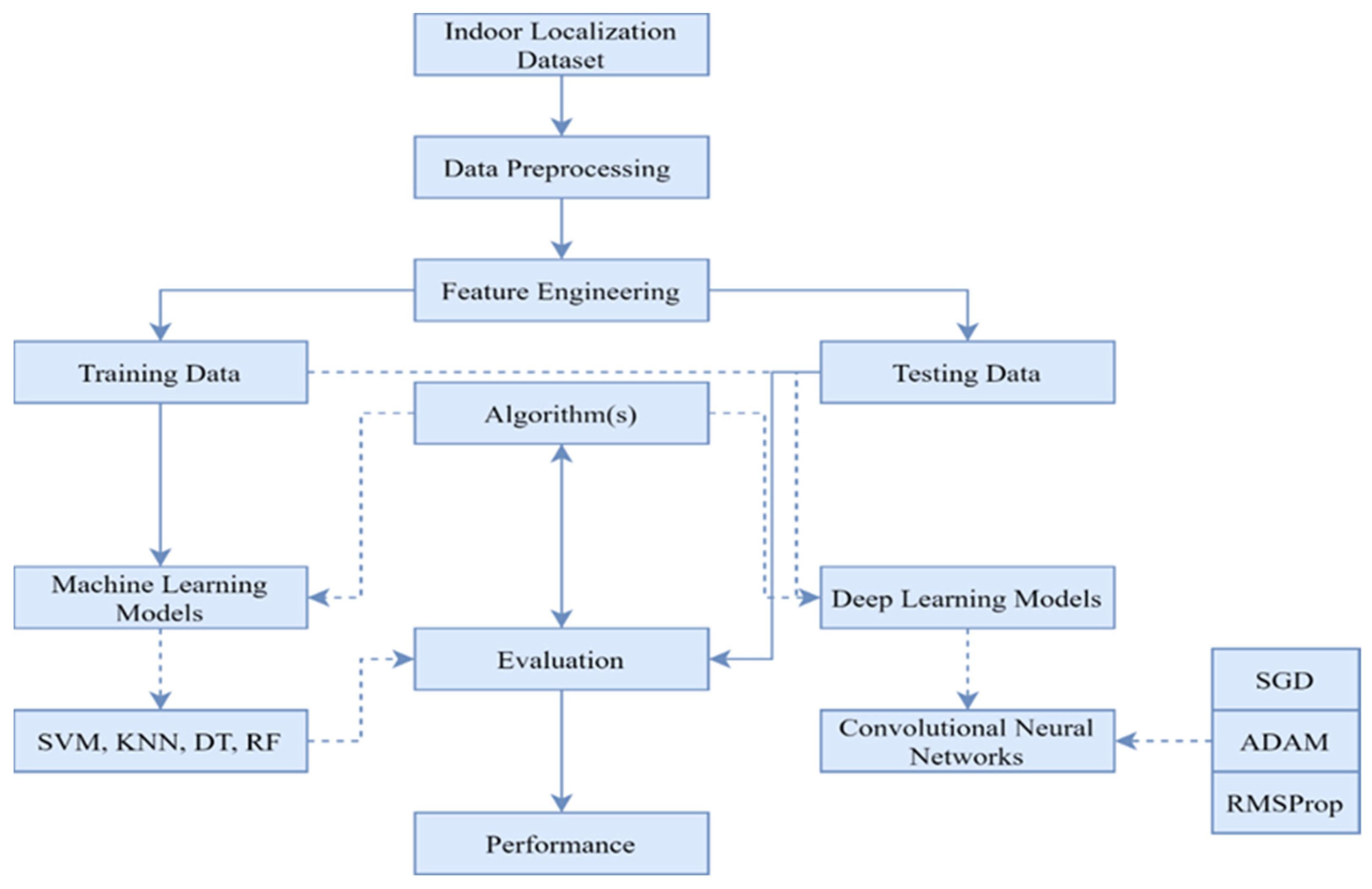
The Digital Twin is then used to create radio maps of the desired location and through the Digital Twin interface, the data are used for practical applications in Flexible Manufacturing Systems. Figure 1 shows the complete methodology of the localization.

Figure 1.
Proposed Framework.
3.1. Convolutional Neural Network
1D Convolutional neural networks are related to the more well-known 2D Convolutional neural networks. Notably, 1D Convolutional Networks are utilized chiefly for texts and 1D signals. Convolution Neural Networks (ConvNets) include filters of varying sizes and forms that convert the original phrase matrix into a lower-dimension matrix. ConvNets are employed to distribute discrete word embedding in text classification. We extract the max value out of a pixel block. It reduces the image so that we can run convolutions and discover patterns on various scales. This operation can also be applied to text. There is only one dimension this time, and we do it on all channels. Convolutions are typical, followed by pooling another convolution, and so on. It allows us to find more dependence in our text. The two procedures discussed before, that is, convolutions and pooling, can be considered feature extractors. Afterwards, we transmit this feature to the system, as a reshaped vector of one row. An addition was made to the traditional work by optimizing the CNN using the following three optimizers.
3.1.1. RMSProp
It reduces the learning rates for Adagard using a moving average that is a squared gradient. It chooses a separate study for each parameter and automatically reduces the learning rate by automatically updating it. The technique uses exponential decay to divide the average learning rate.
β or is the decay term. It will be taken from 0 to 1 in value. gt moves an average gradient of squared.
3.1.2. Adaptive Moment Estimation (Adam)
This technique is used to calculate the learning rate of each parameter by using 1st and 2nd instants. It reduces Adagrad’s learning rates. It is the combination of Adagards. The technique updates the first and second moment’s exponential moveable gradient averages (mt) and squared gradient (vt). The decay rates of these are controlled by β1, β2 β1 [0, 1]; it is shown below.
In particular, the moving averages are zero at first. This leads to instant estimates of zero in the first steps. This initial partition can easily be counteracted, and biased estimates can be achieved.
Finally, as shown below, we update the parameter “θ”
3.1.3. Stochastic Gradient Descent (SGD)
SGD only calculates on a small subset of random data instances instead of computations on the entire dataset—which is redundant and inefficient. Adam is essentially an algorithm to optimize stochastic objective functions through gradients.
One may wonder why we did not simply use the tuned models’ cross-validation score. In the case of the neural network, the tuned neural net’s performance on the validation set is the final indicator of how well the model performs. The general reason for this is that when searching across many sets of hyperparameters, it is possible, by random chance alone, that a set of hyperparameters gives a good cross-validation score/good performance on the cross-validation set. It is a valid concern, especially since most models have more than 2 or 3 hyperparameters to tune. The number of combinations of hyperparameters we can develop is multiplicative, so we have many trials. By choosing to report the tuned model’s performance on a separate test set as the final indicator, we essentially avoid this pitfall of overestimating model performance due to random chance. It is doubtful that a “lucky” model will get lucky both on cross-validation and on the validation and test.
The test set used is the “UJIIndoorLoc_validationData.csv” dataset, which includes separate fingerprints taken by devices that are not in “UJIIndoorLoc_trainingData.csv”. It makes model performances evaluated on the test set quite indicative of real-world performance. It contains examples that the model had not seen during training and examples generated by devices that the model had not seen during training. In the design we have chosen, we validate the model on examples that the model had not seen during training. Then, we are showing the model examples that it had not seen, and examples generated by devices it had not seen. If the optimized model we tune will perform well on the test set, it must be more general to handle new devices, which is good. In the alternative design where we mix the two datasets, we ensure that the validation set and the test set come from the same distribution, so we show the model the devices that are only found in “UJIIndoorLoc_validationData.csv” as well during training. The work suggests that either design choice can be justified, and either one accomplishes the goal of this study, which is to evaluate the feasibility of Wi-Fi signals for indoor positioning.
3.2. Data Preprocessing
No missing values were found. This study used the Wi-Fi fingerprints (columns WAP001 through WAP520) as the features. Each received signal strength value was converted to a positive representation, with 0 representing no signal and 1 to 105 representing weak to strong signals. In any given example, only a few WAPs were detected. Thus, a sparse matrix would more likely represent the data better, which required us to change the no signals representation from 100 s to 0 s.
Since the longitude, latitude, floor, and building number are enough to define a precise location, the space ID, and relative position were not used. Note that unlike in a typical regression or classification problem where there is a single label with two or more values or classes (e.g., “what’s the sales volume of this product”, “what is the object in this image?” or “what is the brand preference of this user, Sony or Acer?”), this problem consists of multiple labels (with each label containing multiple values/classes). A single categorical label was created to handle this called UNIQUE LOCATION, which takes on integer values. As the name implies, the UNIQUE LOCATION label takes on different values for each unique location, defined by the longitude, latitude, floor number, and building ID.
Features were not centered since that would destroy the sparse structure of the data. However, since gradient descent algorithms converge faster with normalized values, the features in the training set for the neural network were normalized to a 0-to-1 range by dividing by 105.
The package to train the neural network required that categorical variables be one-hot-encoded into the dummy variable form. It was conducted for the UNIQUE LOCATION label before neural network training. All features contained numerical values.
3.3. Model Explanation
Neural network classification is a layered architecture inspired by the structure of biological neurons. These layers consist of mathematical constructs designed to process and transform input data through a series of interconnected computations.
The training procedure involves repeatedly cycling through the entire training set, where each complete iteration is called an epoch. After each epoch, the model’s parameters are updated based on the cumulative gradients computed from the batches of training examples, thereby progressively refining the network’s predictions.
- (1)
- Hyperparameters Tuned
- Epochs: This refers to the number of complete passes through the entire training dataset during the model’s training process. It is represented as an integer value.
- Batch_size: This parameter determines the number of samples that are propagated through the neural network at once during the training process. It is an integer value, representing the size of each mini-batch used in the optimization algorithm (Adam, a variant of stochastic gradient descent).
- Hidden_layers: This integer value specifies the number of hidden layers in the neural network architecture.
- Neurons_per_hidden_layer: An integer representing the fixed number of neurons or units present in each hidden layer of the neural network. Note that in this case, the same number of neurons was used for all hidden layers.
- L2_reg_lambda: A floating-point value denoting the regularization strength of the L2 regularization technique, which helps prevent overfitting by adding a penalty term to the loss function.
- Dropout: This float value represents the probability of randomly dropping out (or deactivating) a fraction of neurons during the training process, another regularization technique to reduce overfitting.
All other hyperparameters were left at their default values as specified by the package used for training the neural network models.
- (2)
- Model Tuning and Evaluation
A manual grid search was conducted. The use of cross-validation was avoided due to higher computational cost as well as training time required. As for the best model, we used the hyperparameter values that offer the highest accuracy. To estimate the degree of overfitting, we found the accuracies of the training set, and validating set, subsequently finding the difference between them.
3.4. Machine-Learning Models
For each model type (Random Forest, k-NN, and neural network), we used the following approach to perform our data analysis and model building more systematically.
3.4.1. Random Forest Classifier
This technique is an ensemble method that combines outputs from multiple decision trees. In a single decision tree, overfitting is a major issue. This classifier uses the predicted class of different trees, ultimately reducing overfitting. A random sample of size n is used to construct each unique tree from the training set.
Model Training and Evaluation
A grid search was conducted over the hyperparameters using 10-fold cross-validation. The hyperparameter values that yielded the highest cross-validation accuracy were selected as the optimal model. Additionally, the cross-validation kappa was calculated. To assess overfitting, the differences between the cross-validation scores and the average scores on the training folds were computed. The optimal model was then utilized to predict unique locations in the test set. Subsequently, a reference table was used to convert the predicted unique locations back to their corresponding longitude, latitude, floor number, and building ID. For example, for a unique location value of 1151, the longitude is −7541.26 m, the latitude is 4.86492 × 10⁶ m, the floor number is 2, and the building ID is 1. Finally, the following metrics are reported for the predicted test set locations:
Mean positional error—the Euclidean distance between the actual and predicted positions averaged overall test set examples. A position is defined by longitude and latitude (meters. 25, 50, 75, 95, and 100th percentile of the positional error—also based on the Euclidean distance). It indicates how close the most accurate predictions were and how far away the most inaccurate predictions (100th %ile) were in meters.
Building hit rate—the %age of examples where the predicted building ID was correct.
Floor hit rate—the %age of examples where the predicted floor was correct.
3.4.2. K-Nearest Neighbors Classifier
The K-Nearest Neighbors (K-NN) classifier is a non-parametric algorithm. It makes predictions based on the similarity of the data points. Unlike neural networks, it does not involve parameter learning during the training period or phase. Instead, it relies on the distance matrix to classify the new examples.
The K-NN algorithm calculates the distance between a new data point and all the examples in the training set. The matrices of common distances include the following two types of distances:
- Euclidean Distance.
- Manhattan Distance.
After calculating the distances, this algorithm identifies the closest examples. And then assigns the class label based on majority voting. If there is a tie, then the class of the nearest neighbor is chosen. The K-NN has the following characteristics:
- Simplicity: K-NN is very straightforward. It does not need training explicitly.
- Versatility: It can be applied to both classification and regression tasks.
- Sensitivity: This algorithm is very sensitive in operation. A small variable may lead to overfitting, while a large one may result in underfitting.
3.4.3. Support Vector Machine
Support Vector Machines (SVMs) are very robust algorithms. They are designed for both linear and non-linear classification operations. They identify a hyperplane that maximizes the margin. This is the distance between the hyperplane and the nearest data points from each class. The classes are called Support Vectors.
For a linearly separable dataset, the SVM optimization problem aims to
- Maximize the margin.
- Subject to the constraints.
For non-linear data, SVMs employ kernel functions. Examples of kernel functions are radial basis function and polynomial. These functions map the data into higher-dimensional spaces where a linear decision boundary can be constructed.
3.4.4. Decision Trees
Decision trees classify data by splitting. The splitting of data into sub-sets is based on feature values. Each node in the tree represents a decision rule and terminal nodes which are leaves. The leaves correspond to class labels or predicted values.
During training, the algorithm recursively partitions the dataset. It is carried out by selecting the feature that provides the highest information gain or reduction in impurity such as Gini Index, or entropy. This iterative process continues until a stopping criterion is met, such as a maximum tree depth or a minimum number of samples per leaf node.
The decision trees are intuitive and interpretable. Yet they are prone to overfitting. Techniques like pruning or ensembling are often employed to improve their generalization capabilities.
3.5. Data Analysis
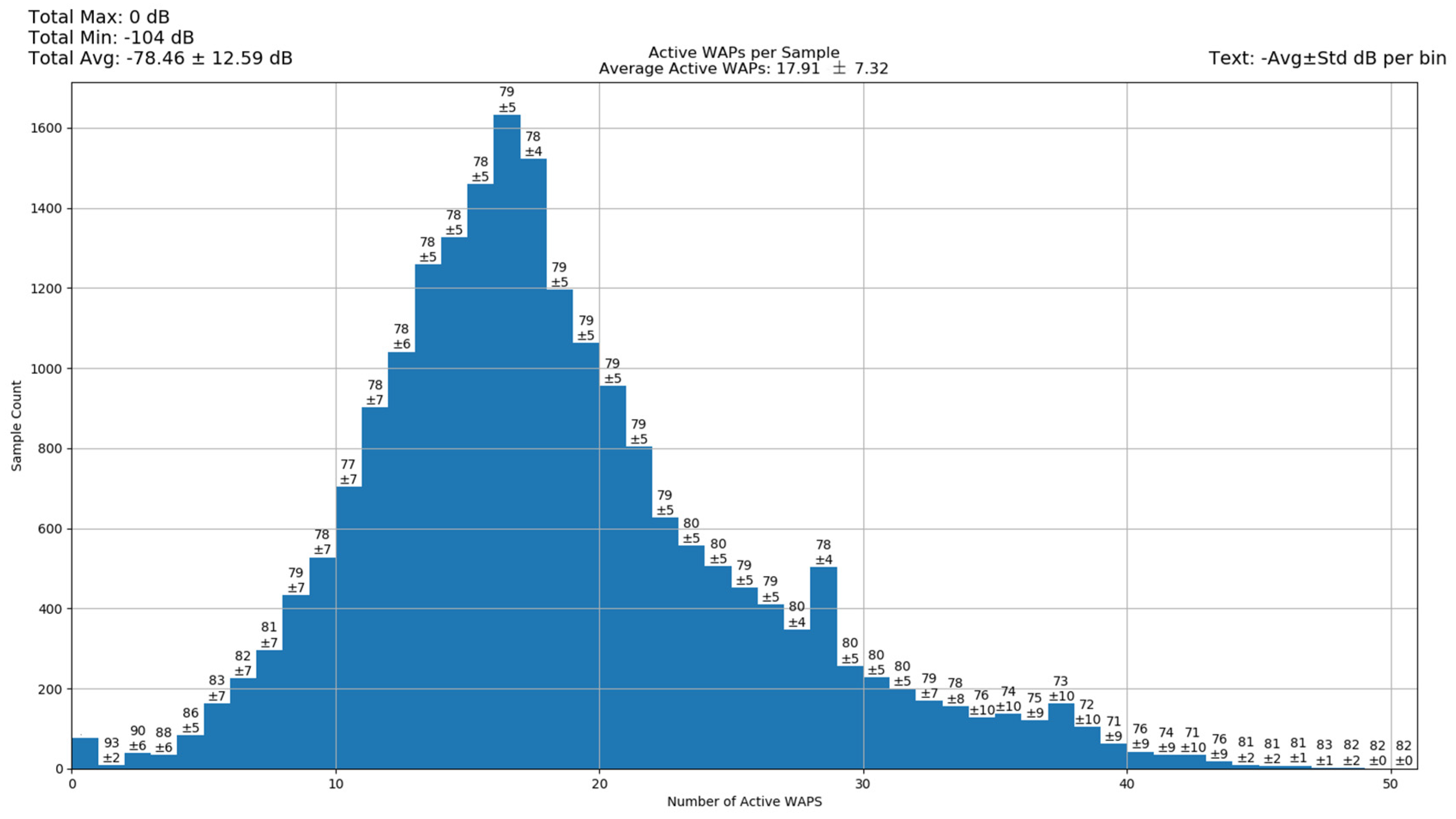
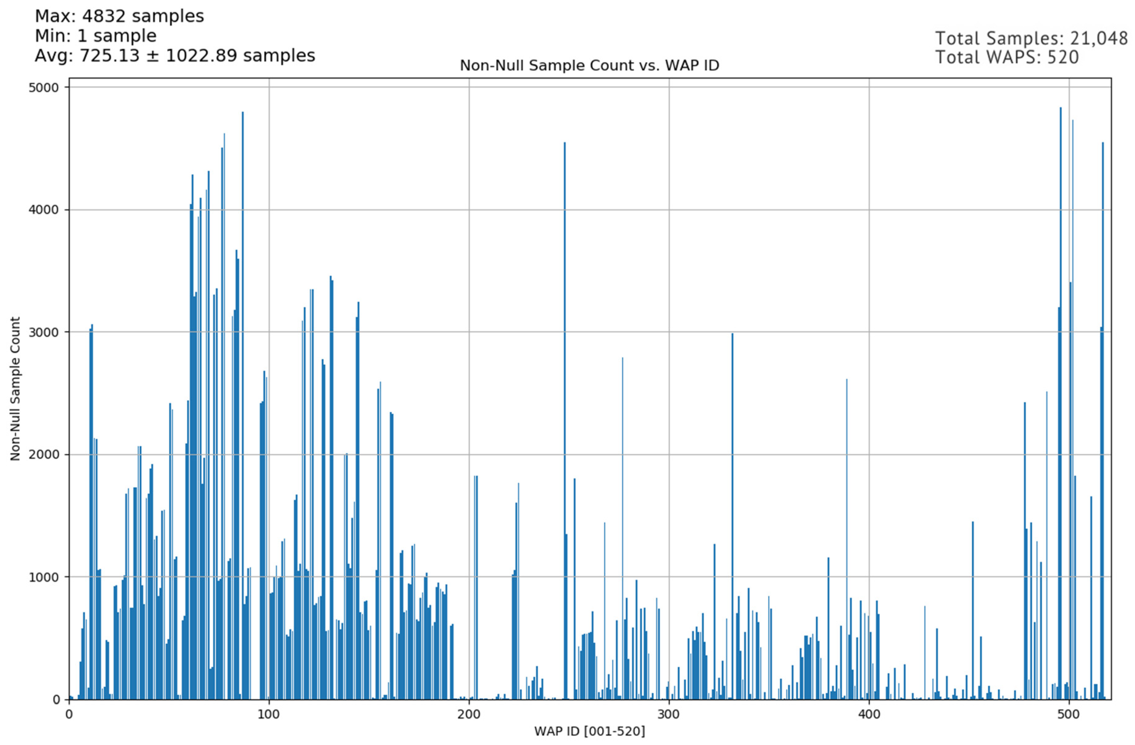
An access point has the potential to cover an area of 10,000 square feet, but for our current discussion, we will rely on the previously mentioned average of 1600 square feet per access point. Figure 2 illustrates the active WAPs per sample.

Figure 2.
Active WAPS per sample [48].
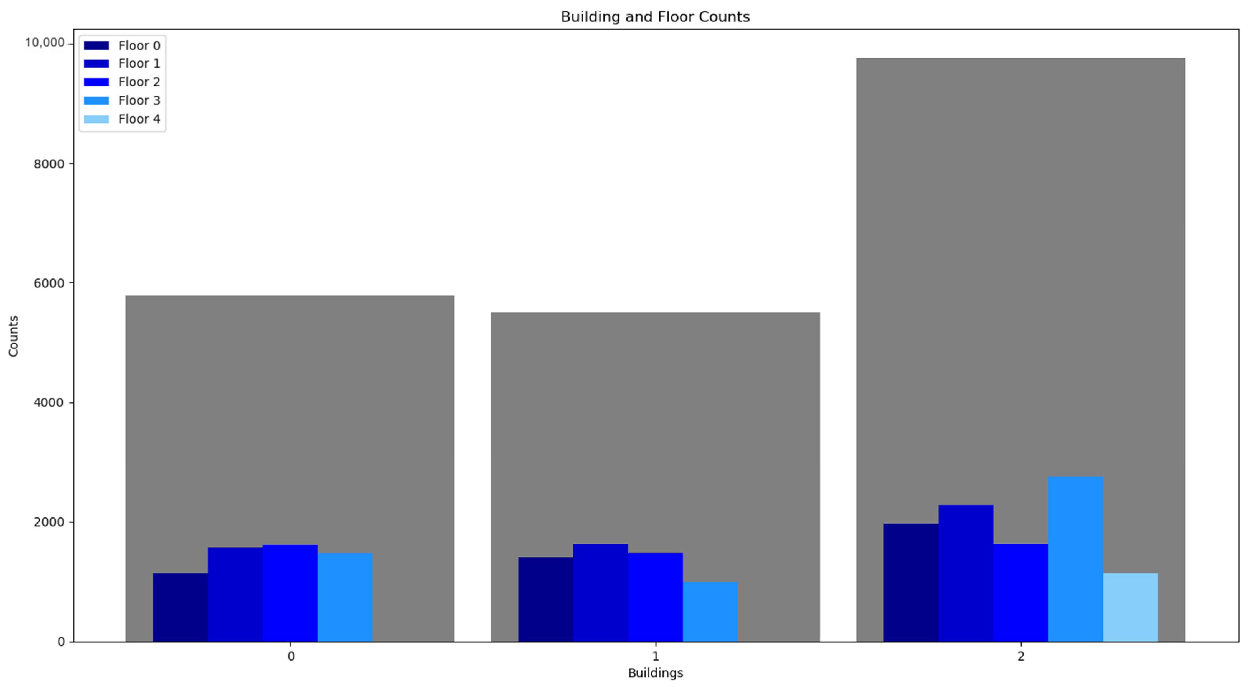
Figure 3 shows the building and floor counts that have been considered in the study.
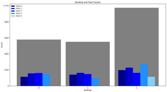
Figure 3.
Floors and Building Counts [48].
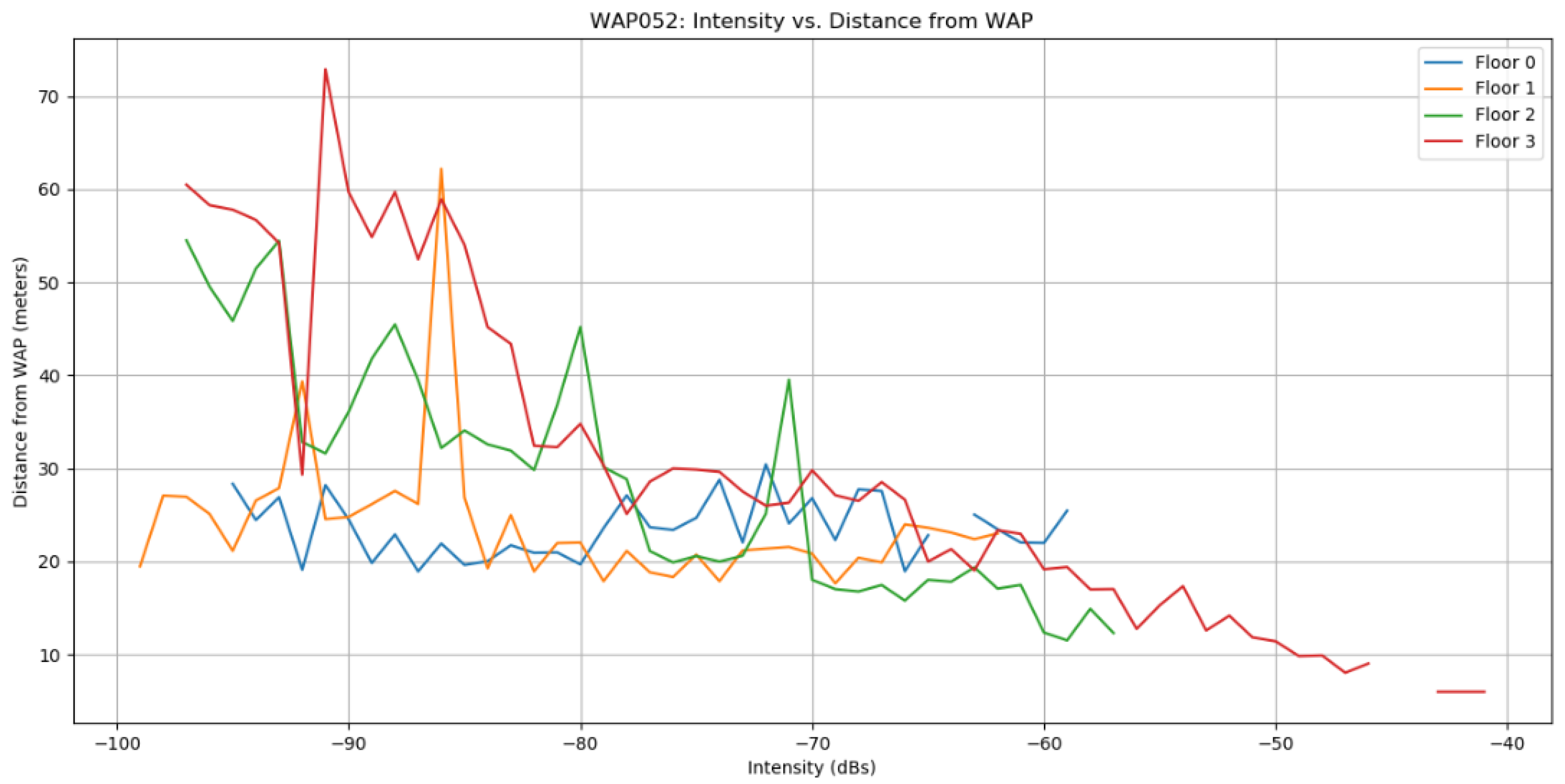
The access points are classified into two types. The first ones are used to communicate via radio and the latter are used to connect to a wired network, like Ethernet or Wi-Fi.
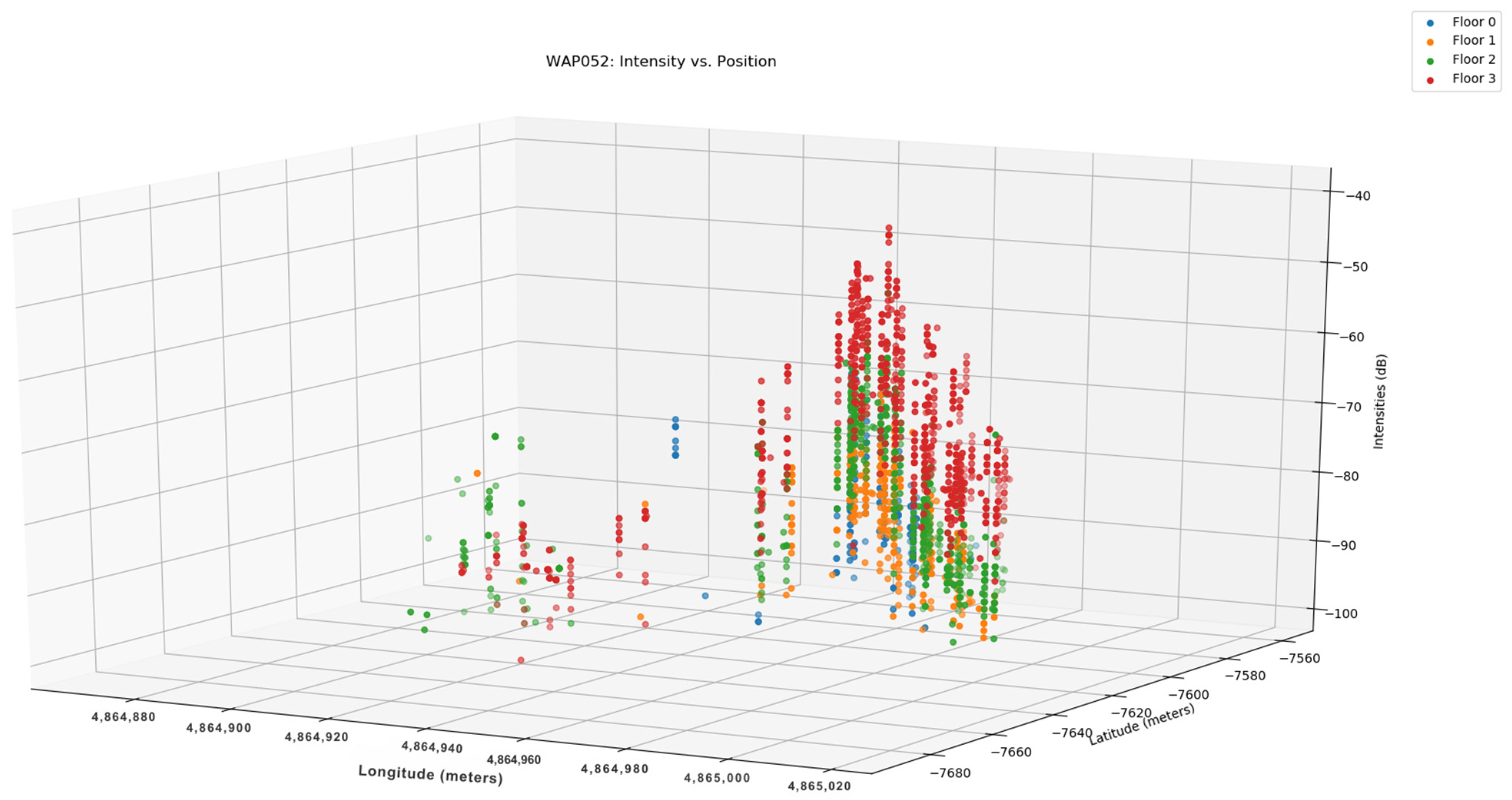
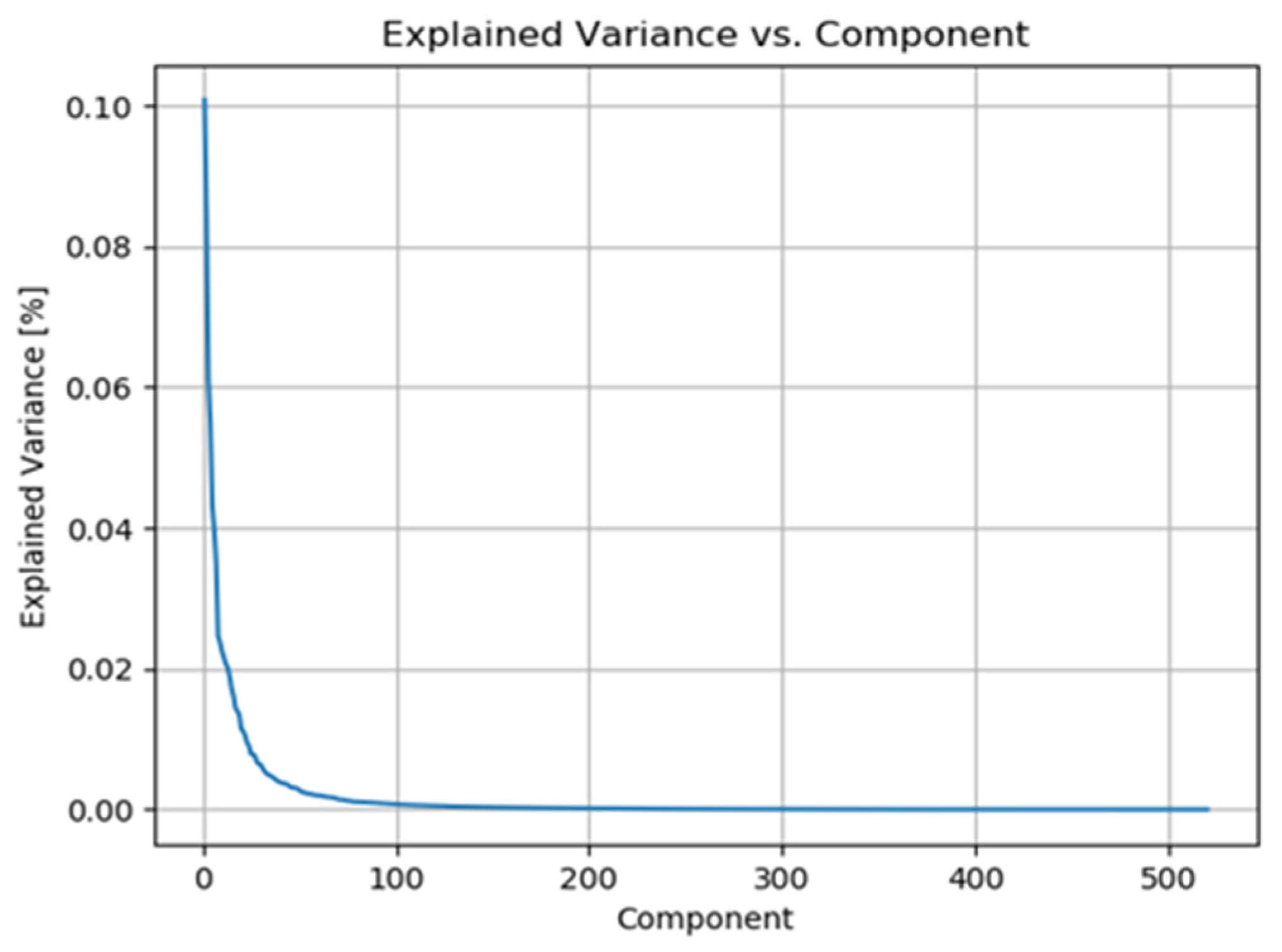
Several factors contribute to a weak Wi-Fi signal, with the primary factor being the distance from the router. Wireless routers and access points can only transmit at low power levels, limiting their effective range to approximately 100 feet indoors to prevent interference with other devices. Figure 4 illustrates the relationship between distance and intensity in WAPs, while Figure 5 displays the radio map in 3D. Both Figure 4 and Figure 5 have the same color configuration. Figure 6 depicts the preprocessing steps taken to separate null values from normal values, and Figure 7 demonstrates the distribution of the dataset.

Figure 4.
Distance Vs Intensity [48].

Figure 5.
Intensity Vs Position 3D [48].

Figure 6.
Data Preprocessing to check null values [48].

Figure 7.
Explained Variance vs. Components [48].
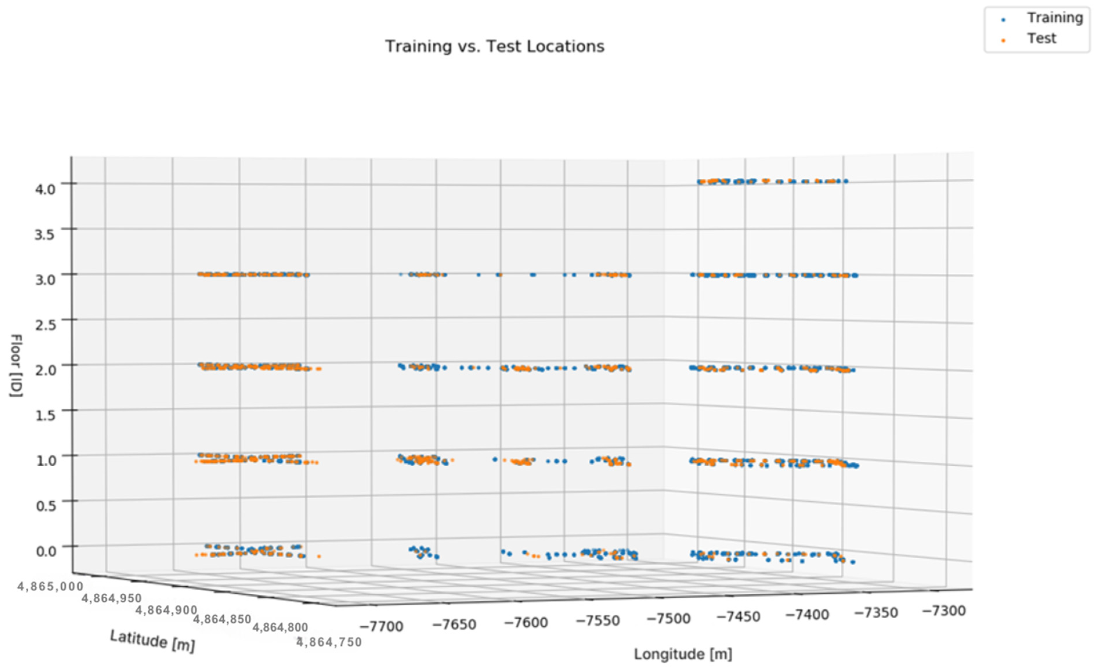
Data have been split into training and testing sets to check the algorithm’s performance. Figure 8 shows the visualization of training and testing data sets.

Figure 8.
Training and Testing Set [48].
3.6. Digital Twin Integration
Achieving a functional Digital Twin of the Flexible Manufacturing System requires the seamless integration of the Wi-Fi-based localization and deep learning prediction models developed in this research. This integration process involves several key steps to create a comprehensive virtual representation and enable remote monitoring, control, and optimization of the physical FMS. The integration steps are as follows:
- A.
- The physical layout of the FMS, including the equipment, workstations, and material handling systems, needs to be captured and digitized. This can be conducted through a combination of techniques, such as 3D laser scanning, photogrammetry, or computer-aided design (CAD) modeling. The resulting 3D virtual environment serves as the foundation for the Digital Twin.
- B.
- Next, the Wi-Fi access points deployed throughout the FMS are mapped to their corresponding locations within the Digital Twin. This spatial alignment allows the real-time localization data from the deep learning models to be seamlessly integrated into virtual representation. As IoT sensors on the physical assets (e.g., Co-Bots, materials, personnel) collect Wi-Fi RSSI data, the deep learning models predict their coordinates, which are then visualized within the Digital Twin.
- C.
- To further enhance the Digital Twin, additional data sources can be integrated, such as production schedules, inventory levels, and equipment status. By combining the localization information with these operational data points, the Digital Twin can provide a holistic view of the FMS, enabling remote monitoring and analysis of the manufacturing processes.
- D.
- The integration of the Digital Twin with optimization algorithms and simulation engines is another crucial step. This allows operators to explore different scenarios, such as changes in product mix, equipment maintenance, or layout reconfiguration, without disrupting the physical system. The Digital Twin can serve as a testbed for evaluating the impact of these changes and identifying the most efficient and effective manufacturing strategies.
- E.
- Finally, the Digital Twin platform should provide intuitive user interfaces and visualization tools to enable real-time monitoring, control, and decision-making. This could include features such as 3D visualizations of the FMS, data dashboards, and predictive analytics to support the optimization of flexible manufacturing operations.
3.7. Reinforcement Learning in Digital Twin
In this research, the Digital Twin was integrated with a deep reinforcement learning (RL) algorithm. It is conducted in order to enhance autonomous navigation. The RL agent was specifically designed for an Automated Guided Vehicle (AGV). The working of the RL agent is as follows:
- a.
- The deep RL algorithm was trained in a simulation environment. This simulation environment was generated from the Digital Twin of the AMP Lab. The agent learned to calculate the optimal trajectories between designated start and endpoints. Furthermore, through the learning, it also understood how to avoid collisions with static and dynamic obstacles. The static obstacles are the FMS and other manufacturing equipment while the dynamic obstacles are humans.
- (1)
- The RL agent reward function incentivized safe navigation and goal achievement. There were penalties for collisions or deviations from efficient paths.
- b.
- Static and dynamic obstacles were incorporated in real time. Using data from IoT sensors and mobile devices, the system recalculated trajectories dynamically to adapt to environmental changes.
- c.
- Wi-Fi RSSI data was processed to provide real-time position tracking with an average error of 1 m. This localization accuracy enabled the RL agent to operate effectively with the aid of a Digital Twin.
3.8. Integration with Industry 4.0 Technologies
The proposed Digital Twin framework integrates seamlessly with key industry 4.0 technologies. This enables enhanced predictive analytics and real-time decision-making capabilities. By leveraging IoT sensors deployed across the manufacturing environment, the framework collects real-time data on equipment status, material flow, and environmental conditions. These data are processed using machine-learning models embedded within the Digital Twin, allowing the system to predict potential failures, optimize production schedules, and adapt to unexpected disruptions.
Real-time decision-making is supported through dynamic dashboards that visualize key performance indicators (KPIs) and suggest optimal actions based on the Digital Twin’s simulations. This integration of Industry 4.0 technologies ensures that the Digital Twin framework not only mirrors the physical system but also enhances operational efficiency and resilience through predictive and adaptive capabilities.
Results demonstrated in our previous paper [49] on the same framework show that the Digital Twin significantly improved FMS performance. Productivity was enhanced by 14.53% compared to conventional methods, energy consumption was reduced by 13.9%, and quality was increased by 15.8% through intelligent machine coordination. The dynamic optimization and closed-loop control capabilities of the Digital Twin significantly improved overall equipment effectiveness.
4. Results
This section shows the results of all machine-learning models, i.e., Random Forests, KNN, Support Vector Machine, Decision Trees, and Convolutional Networks with Optimized Models.
4.1. Random Forests
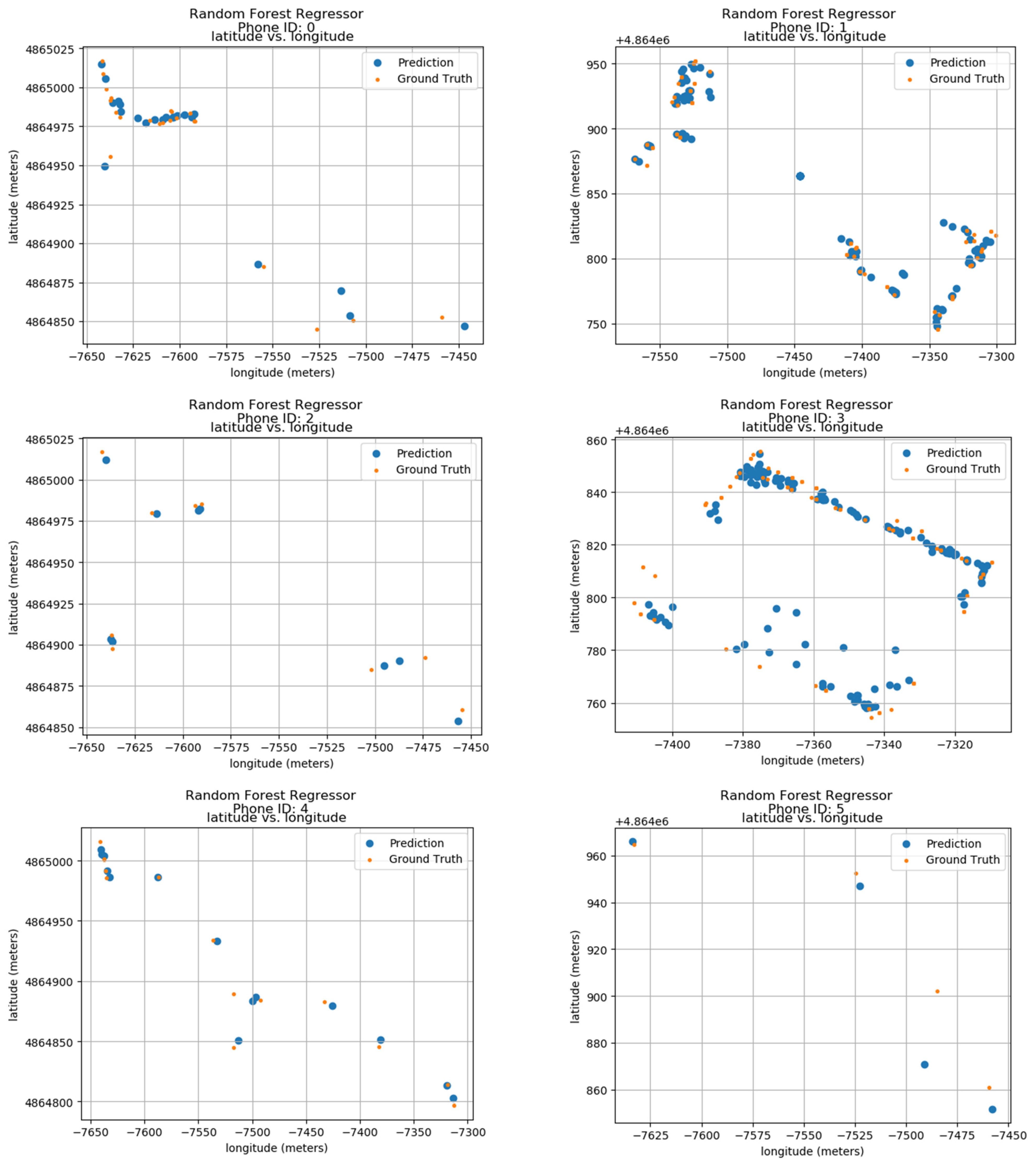
Ground truth and prediction data of the model have been calculated using the longitude and latitude features of the data. The predicted results of 24 phone IDs between 0 and 9 can be seen in the results shown in Figure 9. The results show the phone IDs 0 to 9, the predicted values, as well as the ground values of each one. The ID information is shown on top of each sub-image. The blue color dots show the prediction of the Random Forest Regressor model, and the orange dots show the ground positions in the actual space. The vertical axis of each sub-image’s latitude is in meters and the horizontal axis displays the longitude in meters creating a radio map, where the ID locations throughout the duration are shown. The data show that both predicted and actual locations are within very close proximity showing the accuracy of the model.
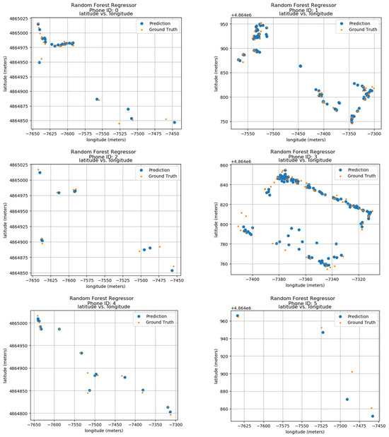
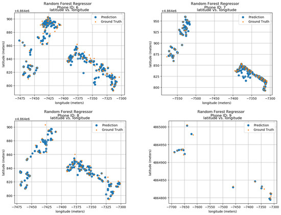
Figure 9.
Localization Results using Random Forests.
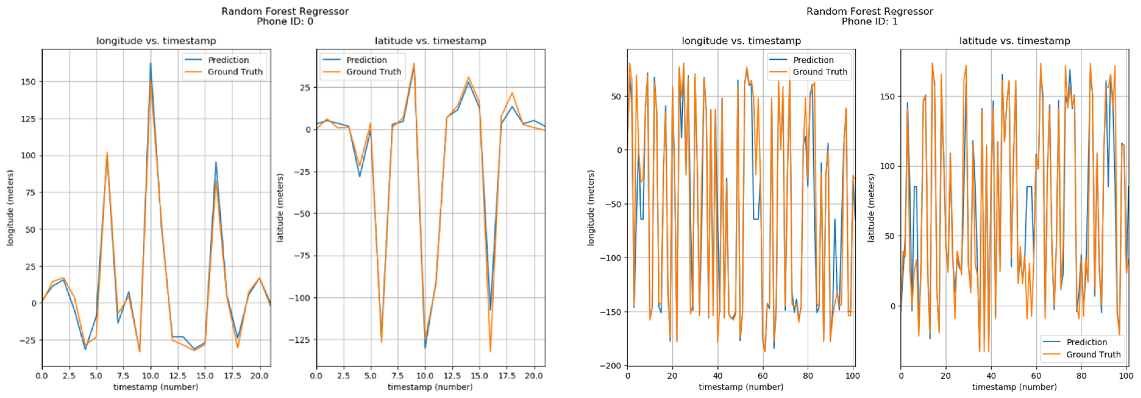
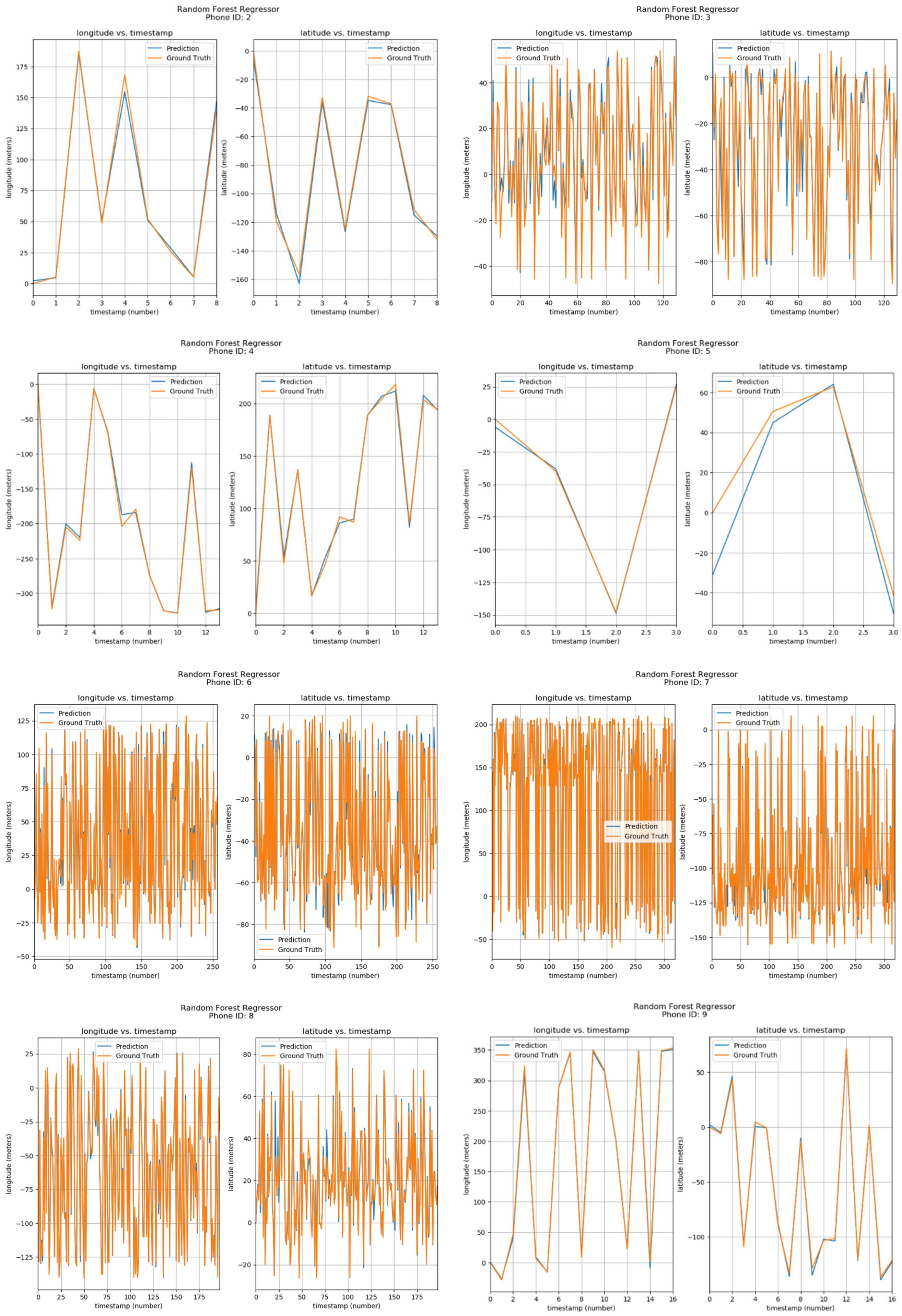
Furthermore, the positions of phone IDs were also predicted by Random Forests using parameters of Longitude/Latitude vs Timestamps. The results can be seen in Figure 10. The corresponding phone ID is shown at the top of each sub-image. Each sub-image has two graphs, one showing the Longitude vs Timestamp data while the other shows the corresponding Latitude. The blue curve shows the predicted values by the Random Forest Regressor model, while the orange one shows the ground locations. From the visualizations, it can be observed that predicted and actual values are quite similar.


Figure 10.
Positioning using Random Forests.
Table 2 shows the complete results of Random Forests with Mean Coordinate Error (MCE), Standard Error (SE), Building % Error (BPE), and Floor % Error (FPE) for each Phone ID.
Table 2.
Performance of Random Forests.
4.2. K-Nearest Neighbors
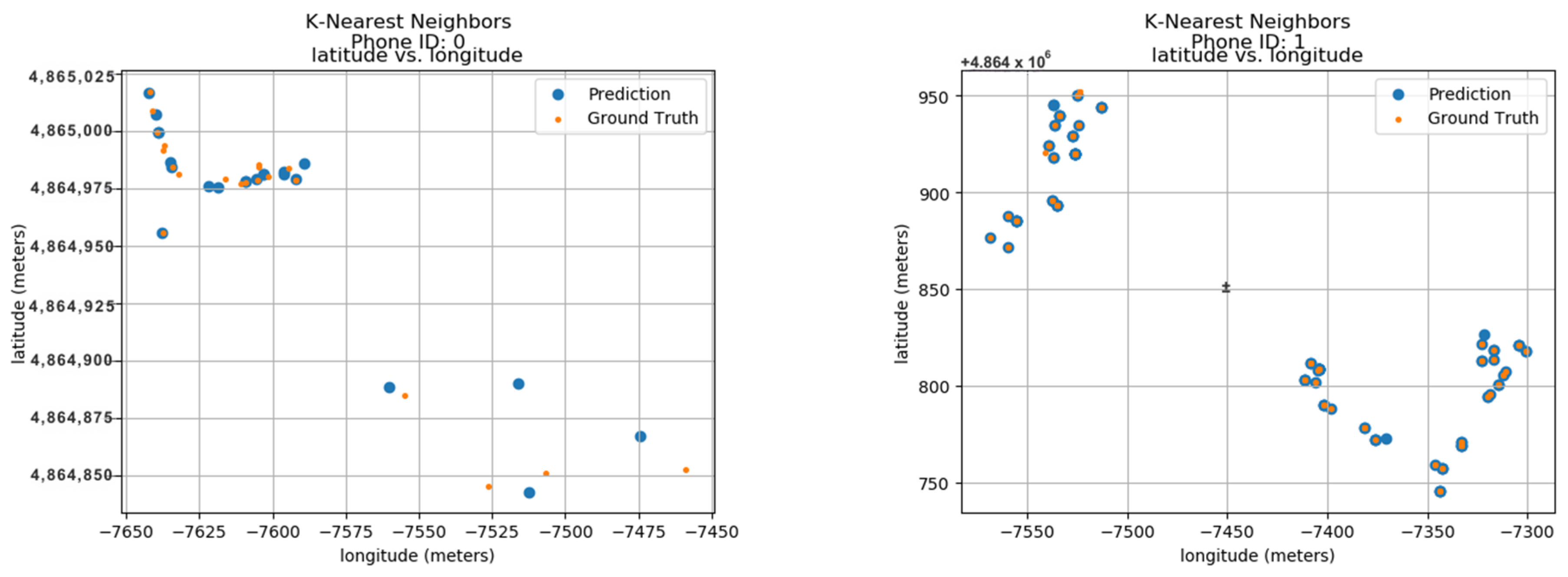
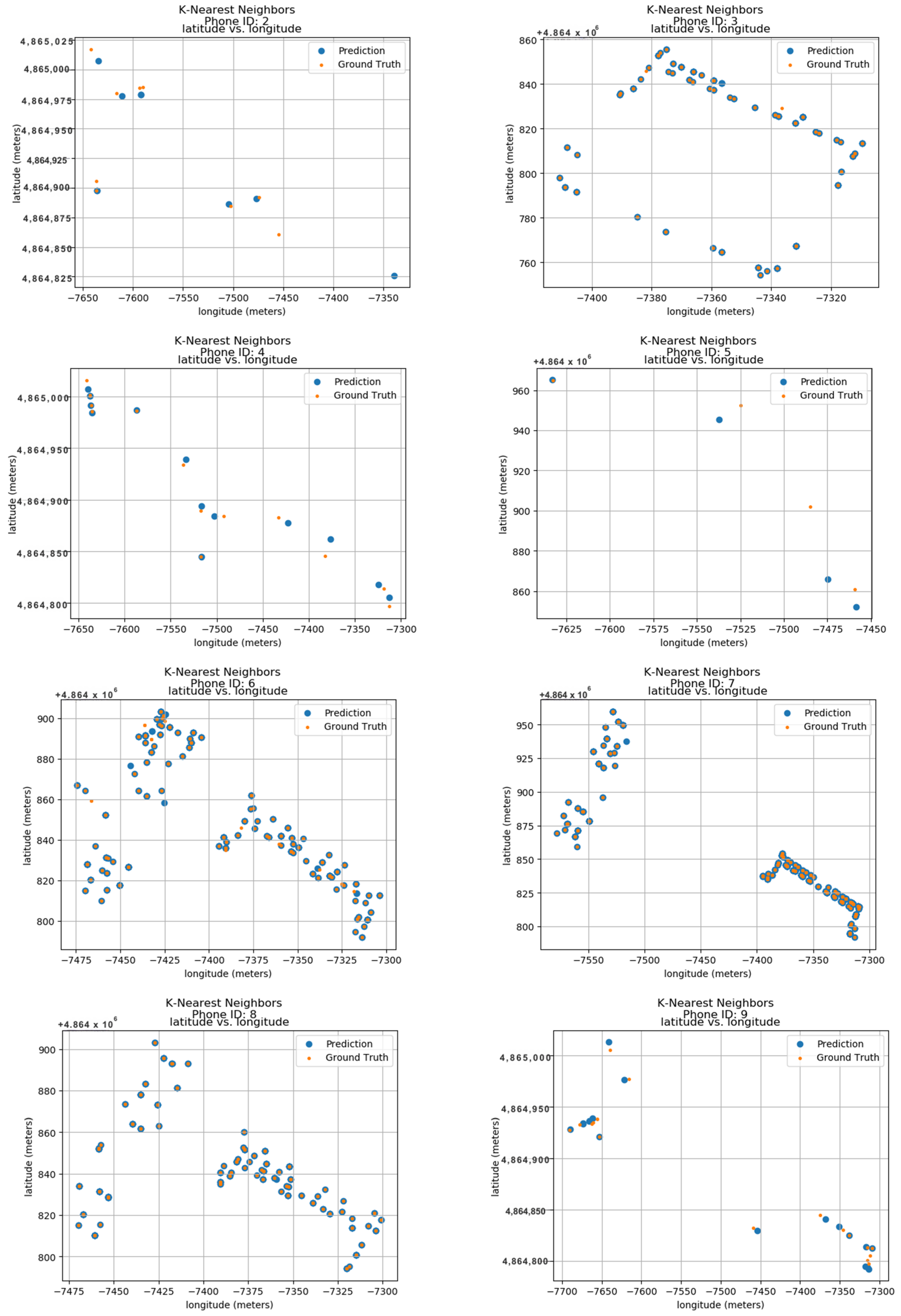
To validate the model’s performance, the research was compared to its predicted locations with the actual ground truth data. These ground truth data are based on the longitude and latitude features within the dataset. Figure 11 displays the predicted results for 24 unique phone IDs, ranging from 0 to 9. Each sub-image within the figure showcases the ground truth and predicted locations for a single phone ID. The phone ID is conveniently positioned at the top of each sub-image for easy reference. The blue dots represent the locations predicted by the K-Nearest Neighbors Forest Regressor model, while the orange dots depict the actual ground positions in real space. Each sub-image utilizes a radio map format, where the vertical axis represents latitude in meters and the horizontal axis represents longitude in meters. This layout allows for the visualization of phone ID locations throughout the data collection period. The close proximity between the predicted blue dots and the actual orange dots demonstrates the model’s accuracy in pinpointing phone locations. This visual confirmation highlights the model’s effectiveness in utilizing longitude and latitude features for indoor localization.
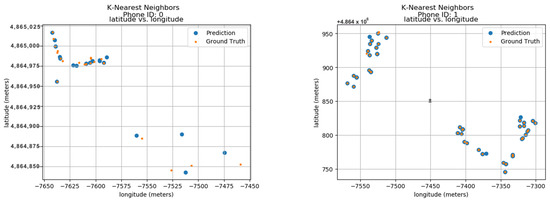
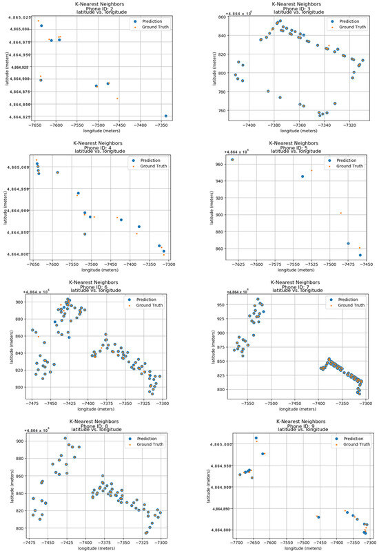
Figure 11.
Localization using KNN.
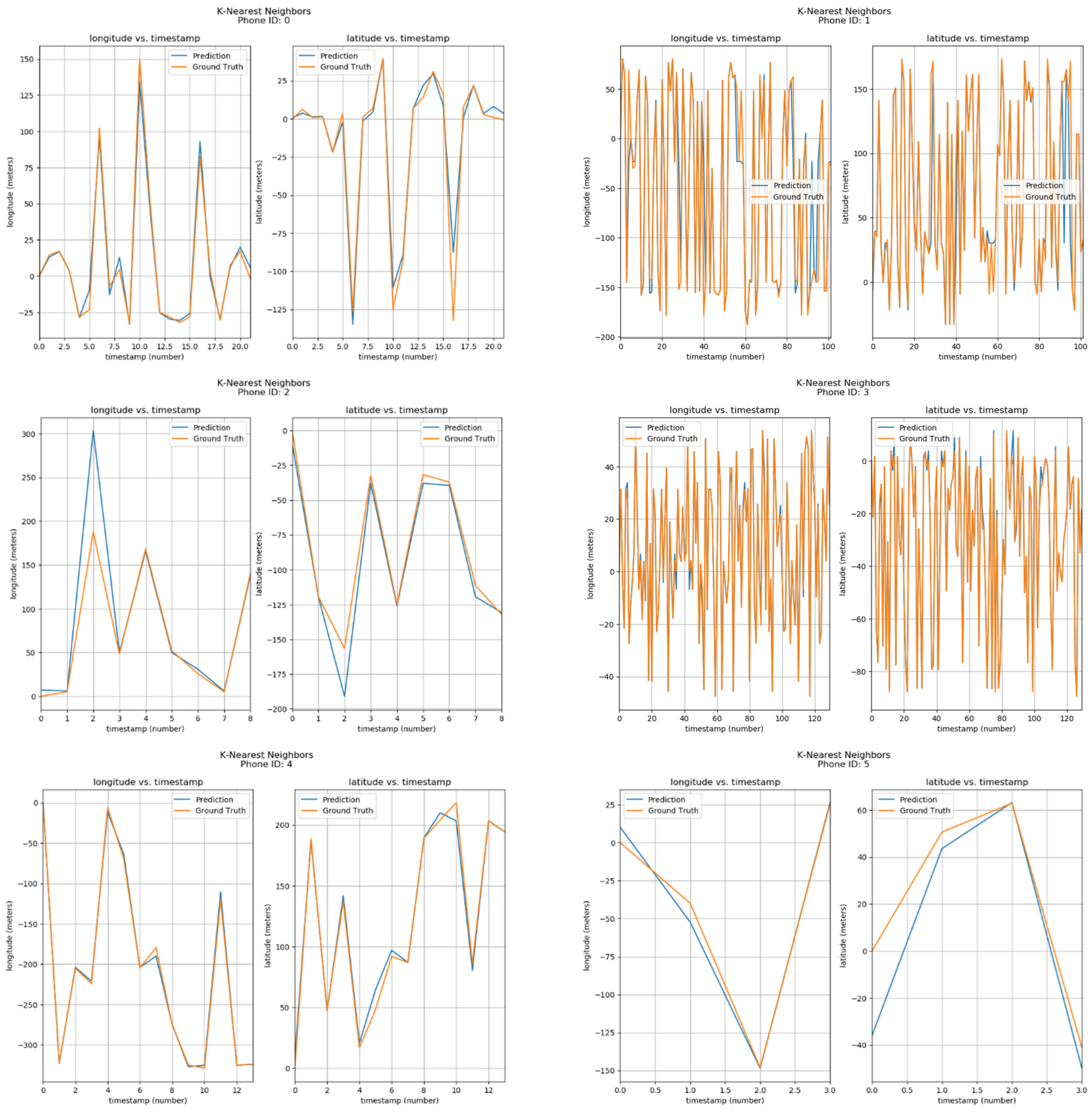
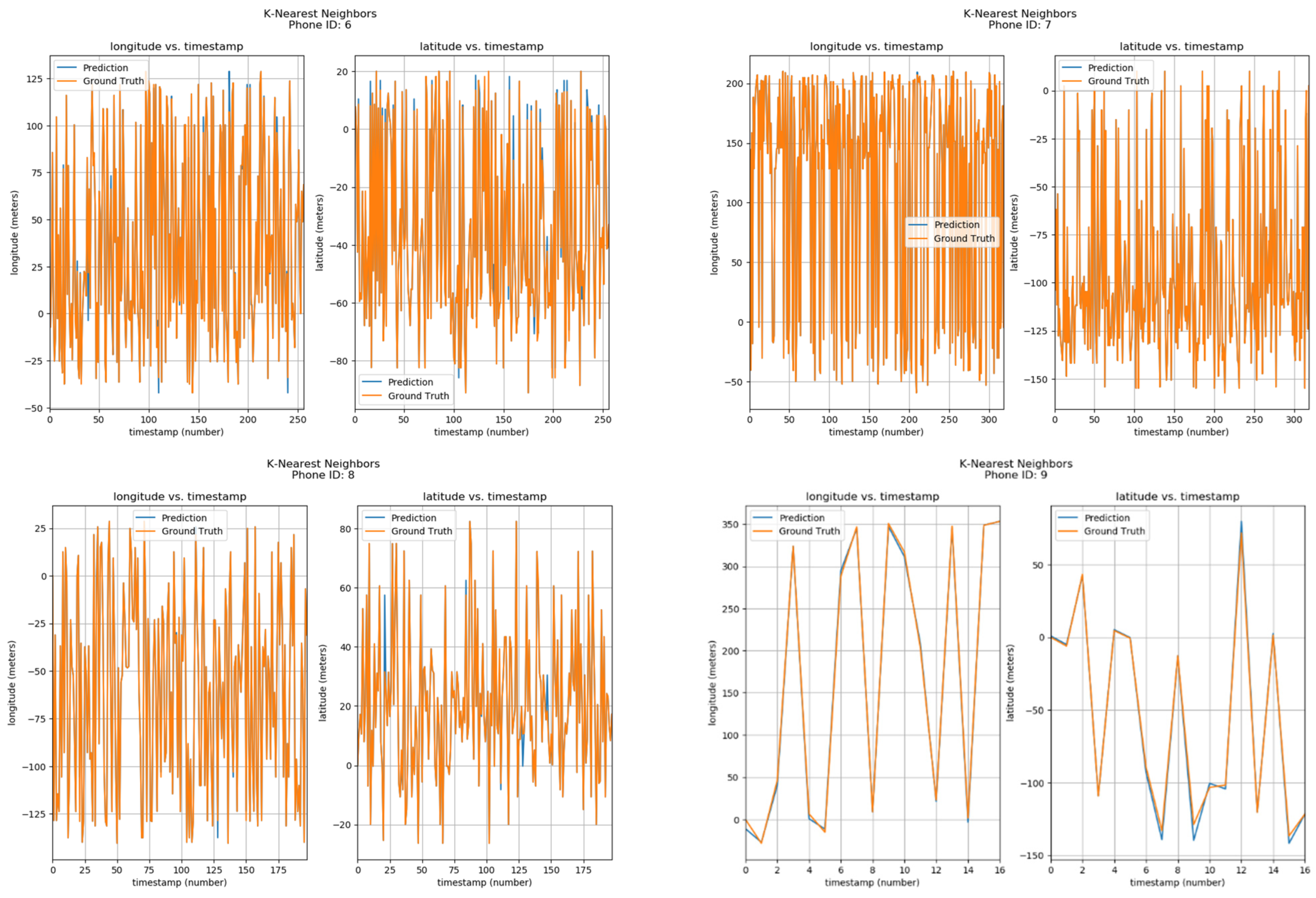
Furthermore, the positions of phone IDs were also predicted by K-Nearest Neighbor using parameters of Longitude/Latitude vs Timestamps. The results can be seen in Figure 12. The corresponding phone ID is shown at the top of each sub-image. Each sub-image has two graphs, one showing the Longitude vs Timestamp data while the other shows the corresponding Latitude. The blue curve shows the predicted values by the K-Nearest Neighbor model, while the orange one shows ground locations. From the visualizations, it can be observed that predicted and actual values are quite similar.


Figure 12.
Positioning using KNN.
Table 3 shows the complete results of KNN with Mean Coordinate Error (MCE), Standard Error (SE), Building % Error (BPE), and Floor % Error (FPE) for each Phone ID.
Table 3.
Performance of KNN.
4.3. Support Vector Machine
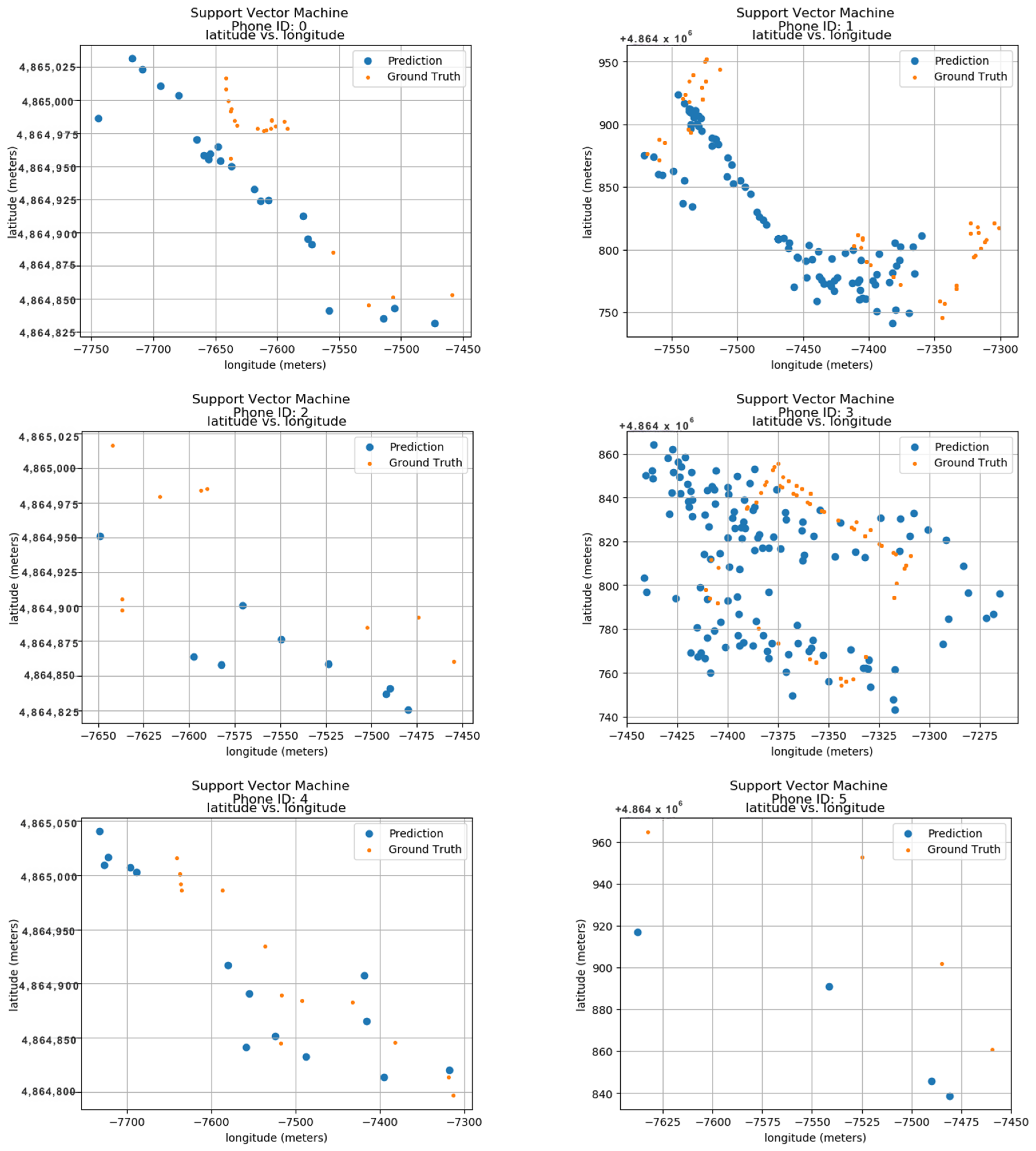
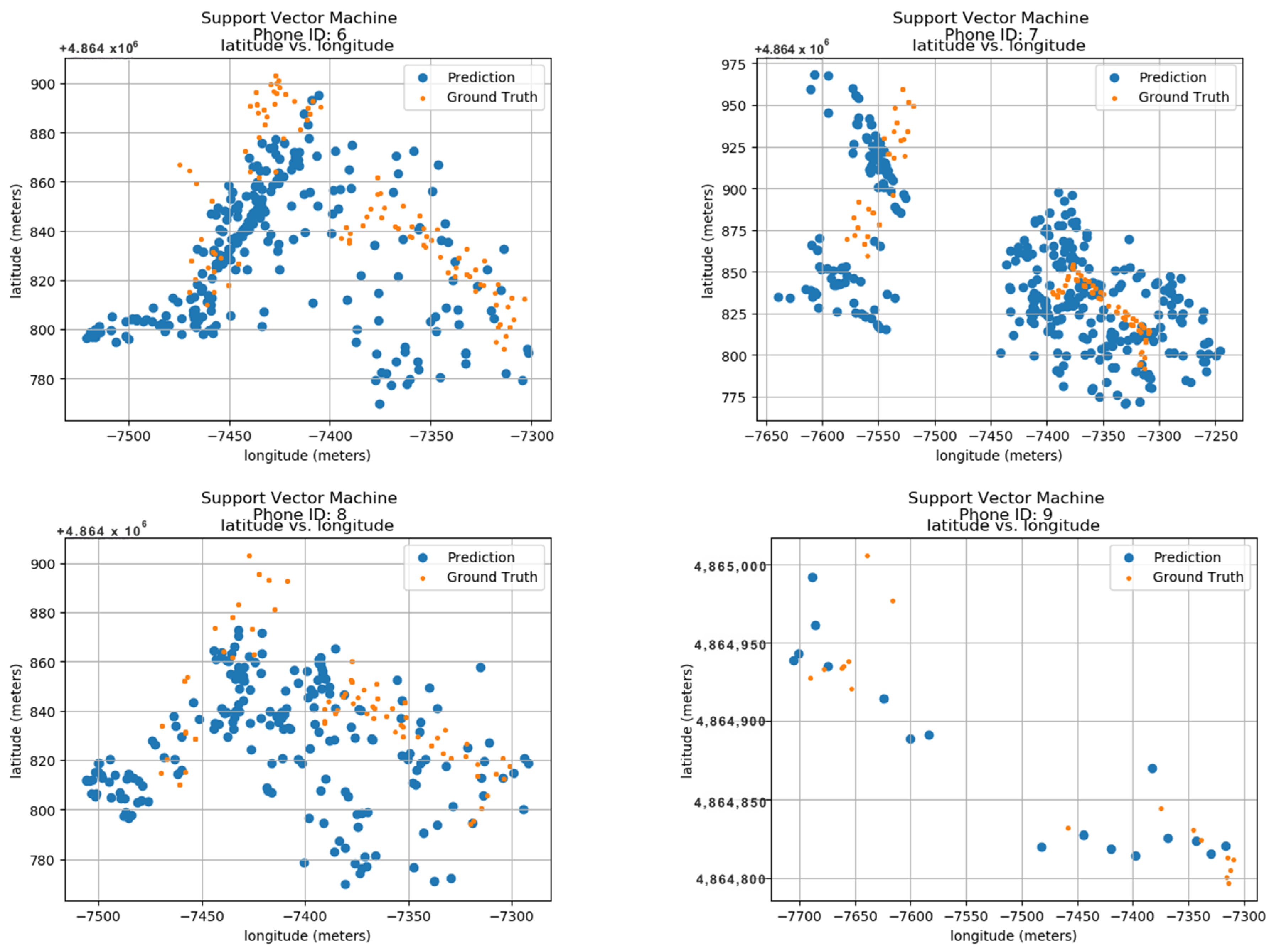
To evaluate the model’s performance, the outcomes were compared to their predicted locations along with the actual ground truth data. These ground truth data are based on the longitude and latitude features within the dataset. Figure 13 displays the predicted results for 24 unique phone IDs, ranging from 0 to 9. Each sub-image within the figure shows the ground truth and predicted locations for a single phone ID. The phone ID is conveniently positioned at the top of each sub-image for easy reference. The blue dots represent the locations predicted by the Support Vector Machine model, while the orange dots depict the actual ground positions in real space. Each sub-image utilizes a radio map format, where the vertical axis represents latitude in meters and the horizontal axis represents longitude in meters. This layout allows for the visualization of phone ID locations throughout the data collection period. The close proximity between the predicted blue dots and the actual orange dots demonstrates the model’s accuracy in pinpointing phone locations. This visual confirmation highlights the model’s effectiveness in utilizing longitude and latitude features for indoor localization.


Figure 13.
Localization using SVM.
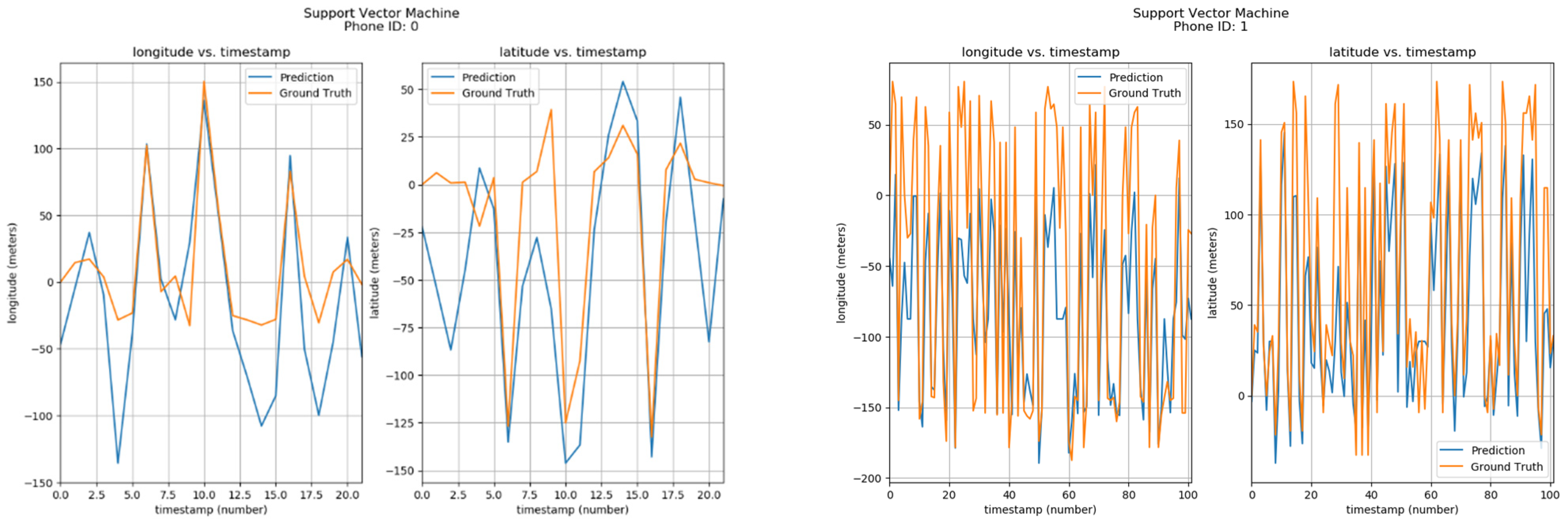
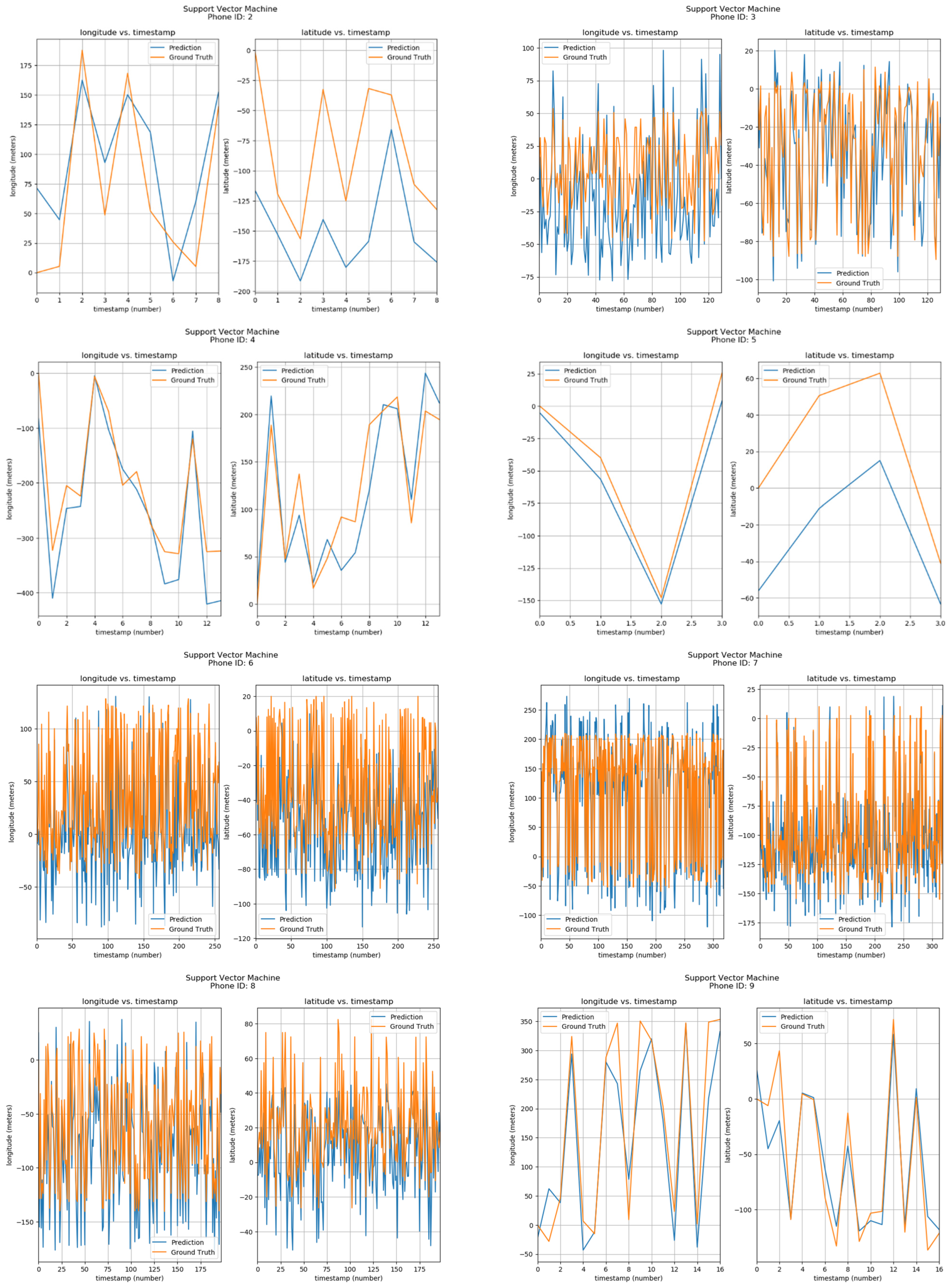
Furthermore, the positions of phone IDs were also predicted by the Support Vector Machine using parameters of Longitude/Latitude vs Timestamps. The results can be seen in Figure 14. The corresponding phone ID is shown at the top of each sub-image. Each sub-image has two graphs, one showing the Longitude vs Timestamp data while the other shows the corresponding Latitude. The blue curve shows the predicted values by the Support Vector Machine model, while the orange one shows ground locations. From the visualizations, it can be observed that predicted and actual values are quite similar.

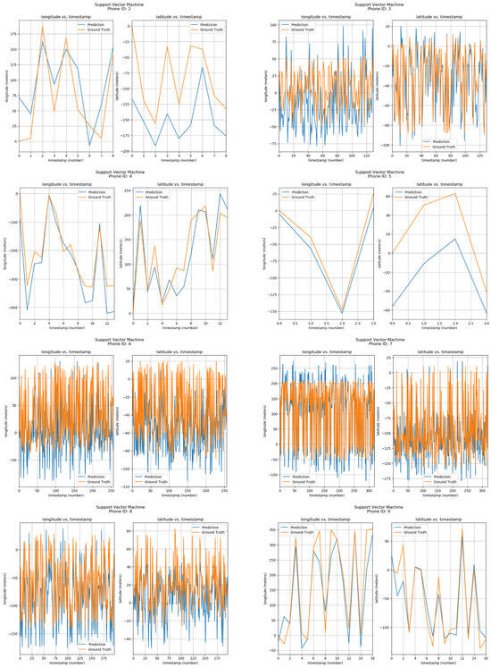
Figure 14.
Positioning using SVM.
Table 4 shows the complete results of SVM with Mean Coordinate Error (MCE), Standard Error (SE), Building % Error (BPE), and Floor % Error (FPE) for each Phone ID.
Table 4.
Performance of SVM.
4.4. Decision Trees
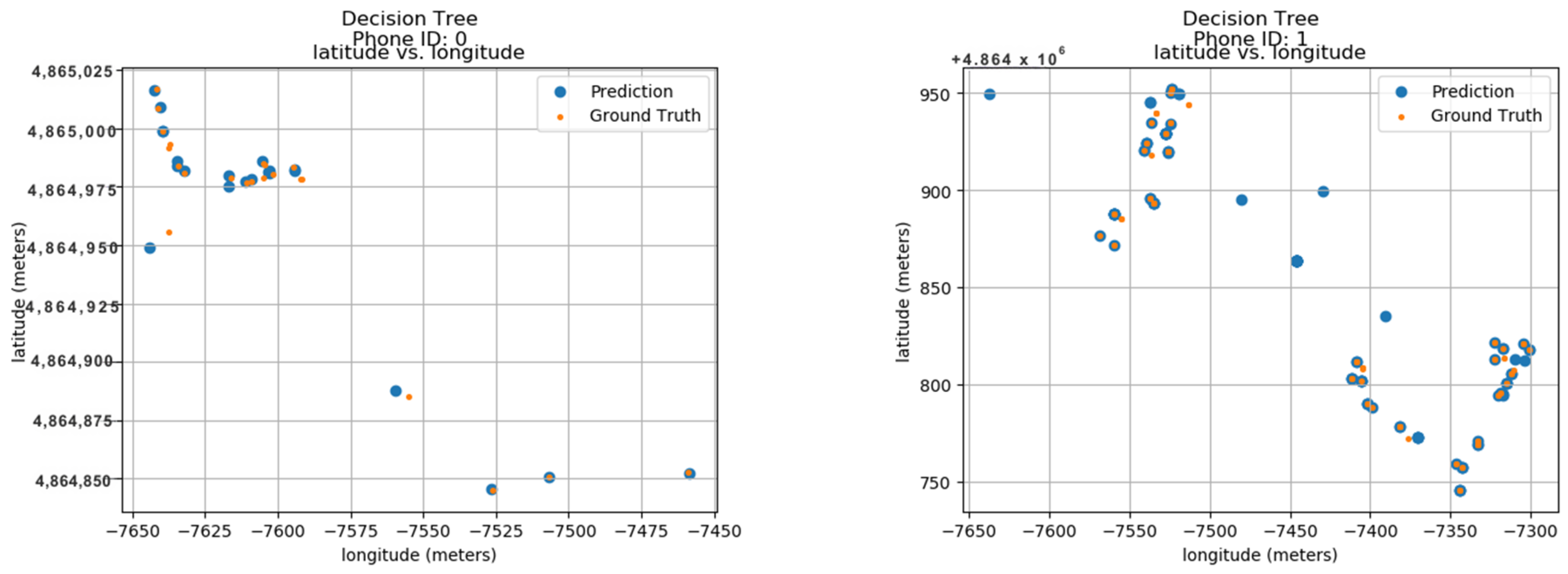
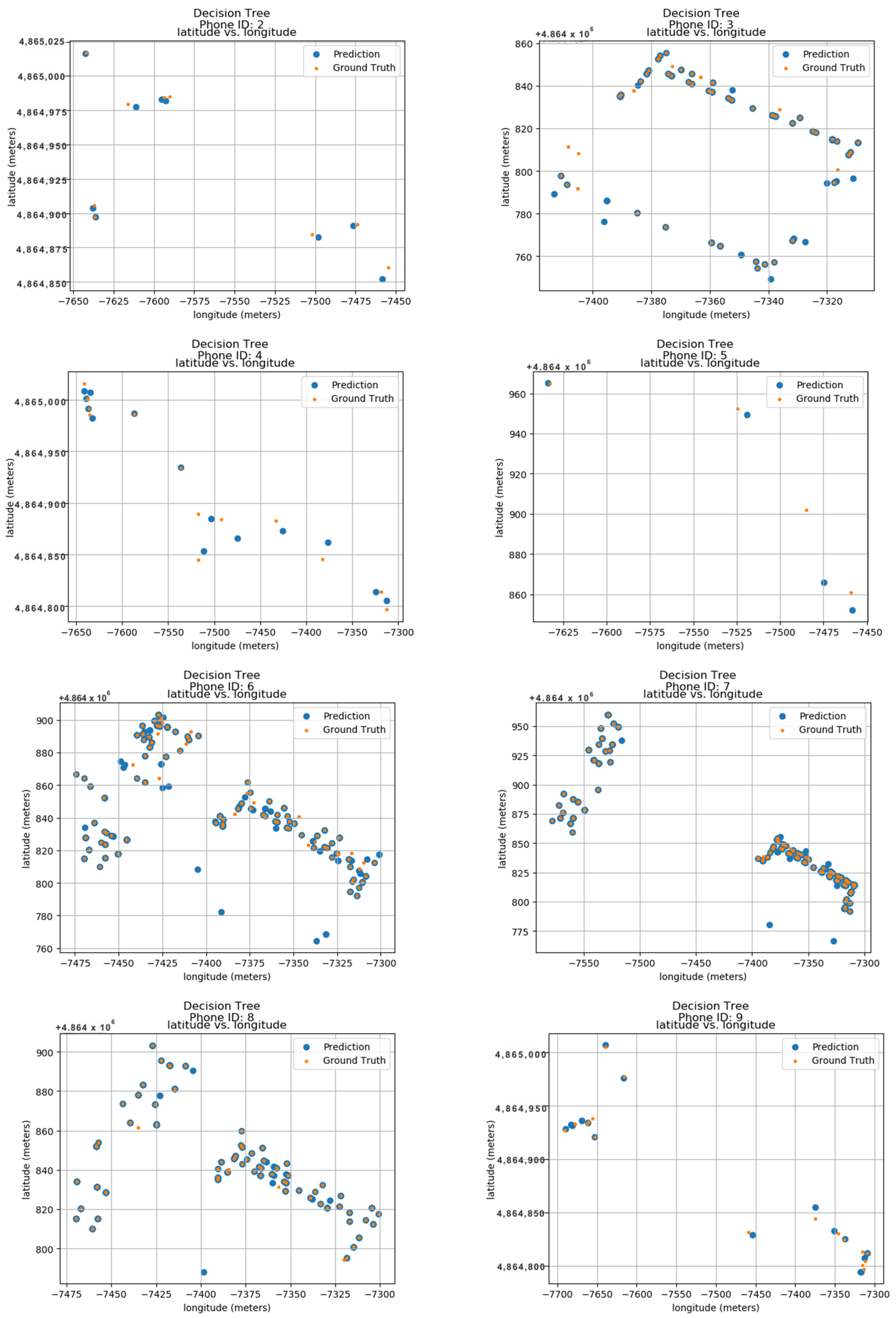
To establish the model’s performance, the calculated values were compared to their predicted locations with the actual ground truth data. These ground truth data are based on the longitude and latitude features within the dataset. Figure 15 displays the predicted results for 24 unique phone IDs, ranging from 0 to 9. Each sub-image within the figure shows the ground truth and predicted locations for a single phone ID. The phone ID is conveniently positioned at the top of each sub-image for easy reference. The blue dots represent the locations predicted by the Decision Tree model, while the orange dots depict the actual ground positions in real space. Each sub-image utilizes a radio map format, where the vertical axis represents latitude in meters and the horizontal axis represents longitude in meters. This layout allows for the visualization of phone ID locations throughout the data collection period. The close proximity between the predicted blue dots and the actual orange dots demonstrates the model’s accuracy in pinpointing phone locations. This visual confirmation highlights the model’s effectiveness in utilizing longitude and latitude features for indoor localization.
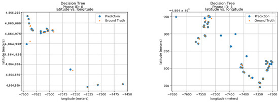
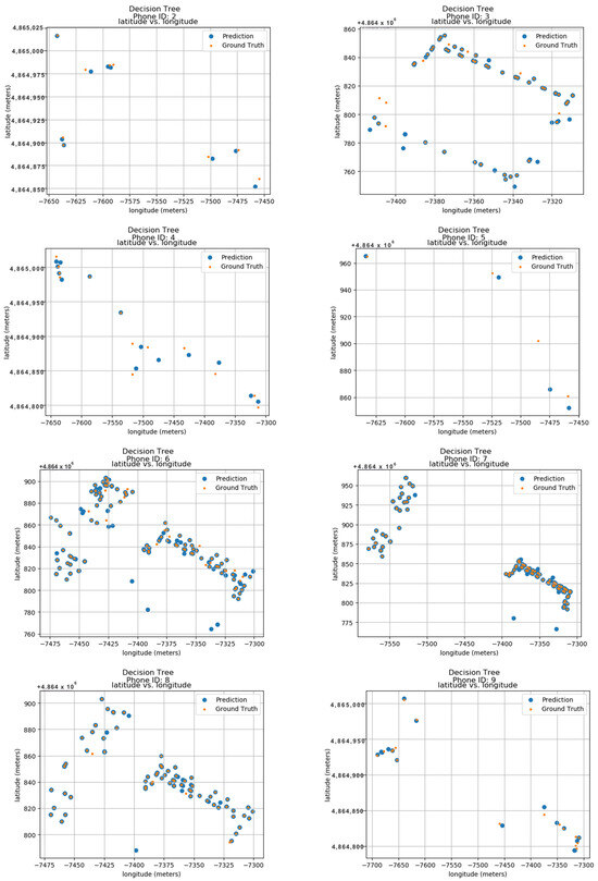
Figure 15.
Decision Trees.
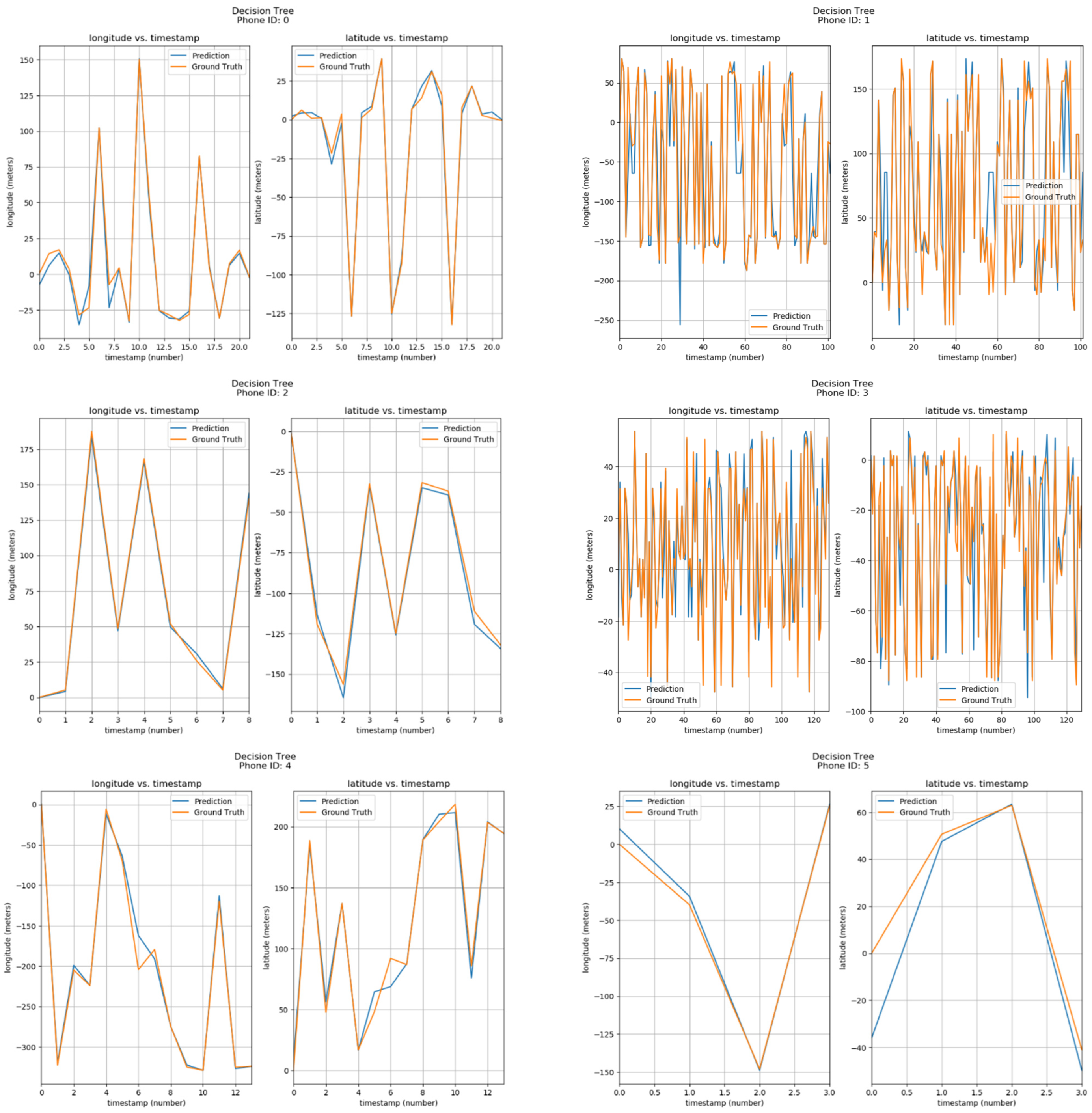
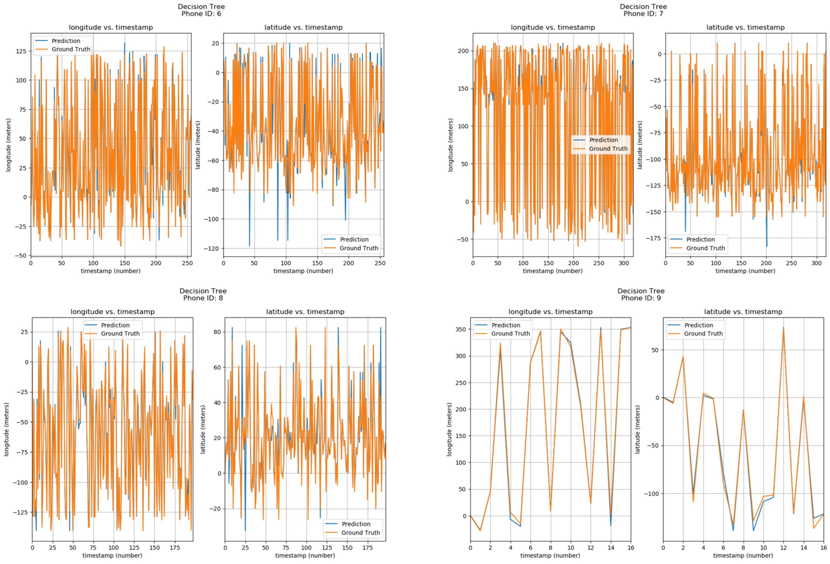
Furthermore, the positions of phone IDs were also predicted by the Decision Tree using parameters of Longitude/Latitude vs Timestamps. The results can be seen in Figure 16. The corresponding phone ID is shown at the top of each sub-image. Each sub-image has two graphs, one showing the Longitude vs Timestamp data while the other shows the corresponding Latitude. The blue curve shows the predicted values by the Decision Tree model, while the orange one shows ground locations. From the visualizations, it can be observed that predicted and actual values are quite similar. Table 5 showcases the error metrics associated with decision tree technique.


Figure 16.
Positioning using Decision Trees.
Table 5.
Performance of Decision Trees.
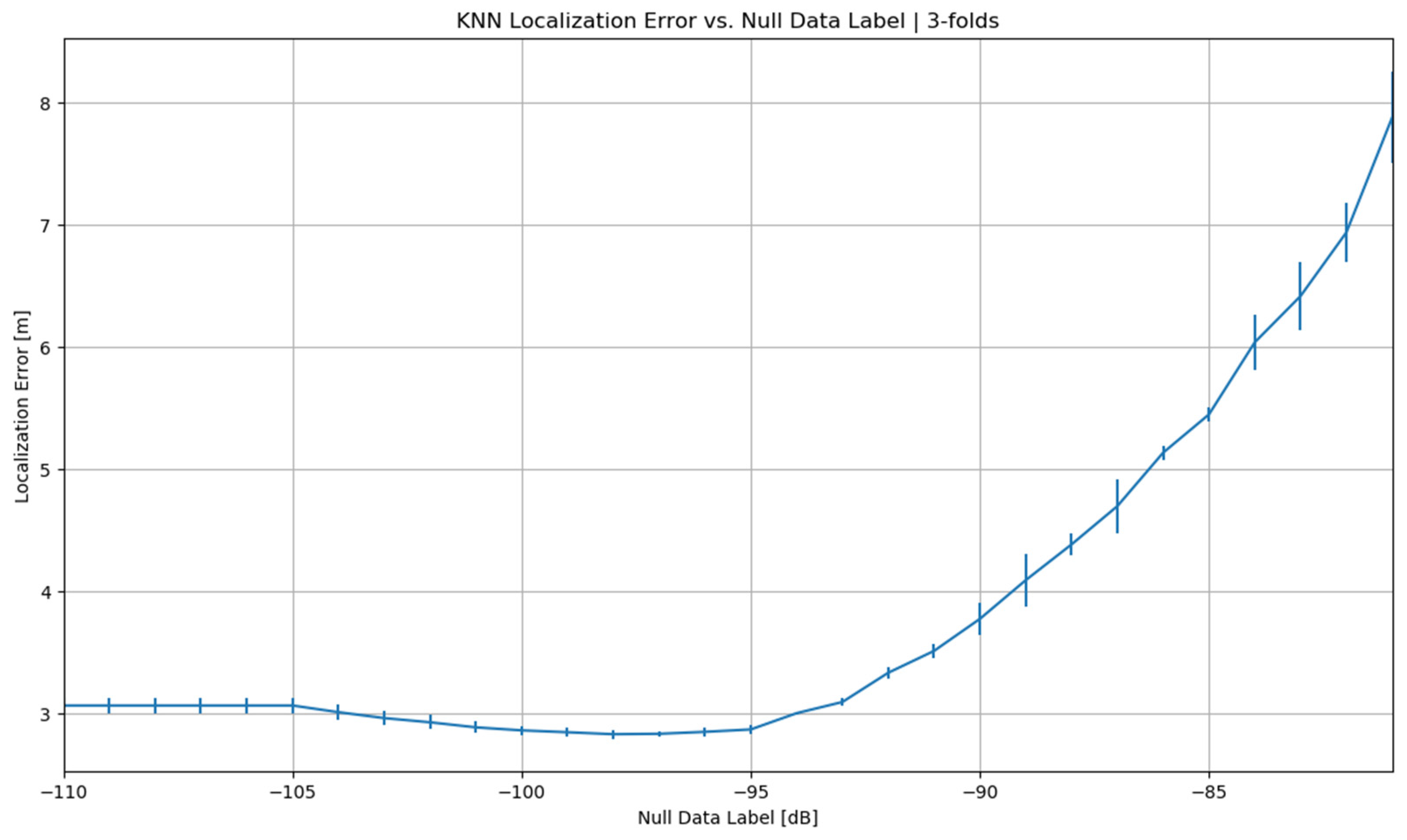
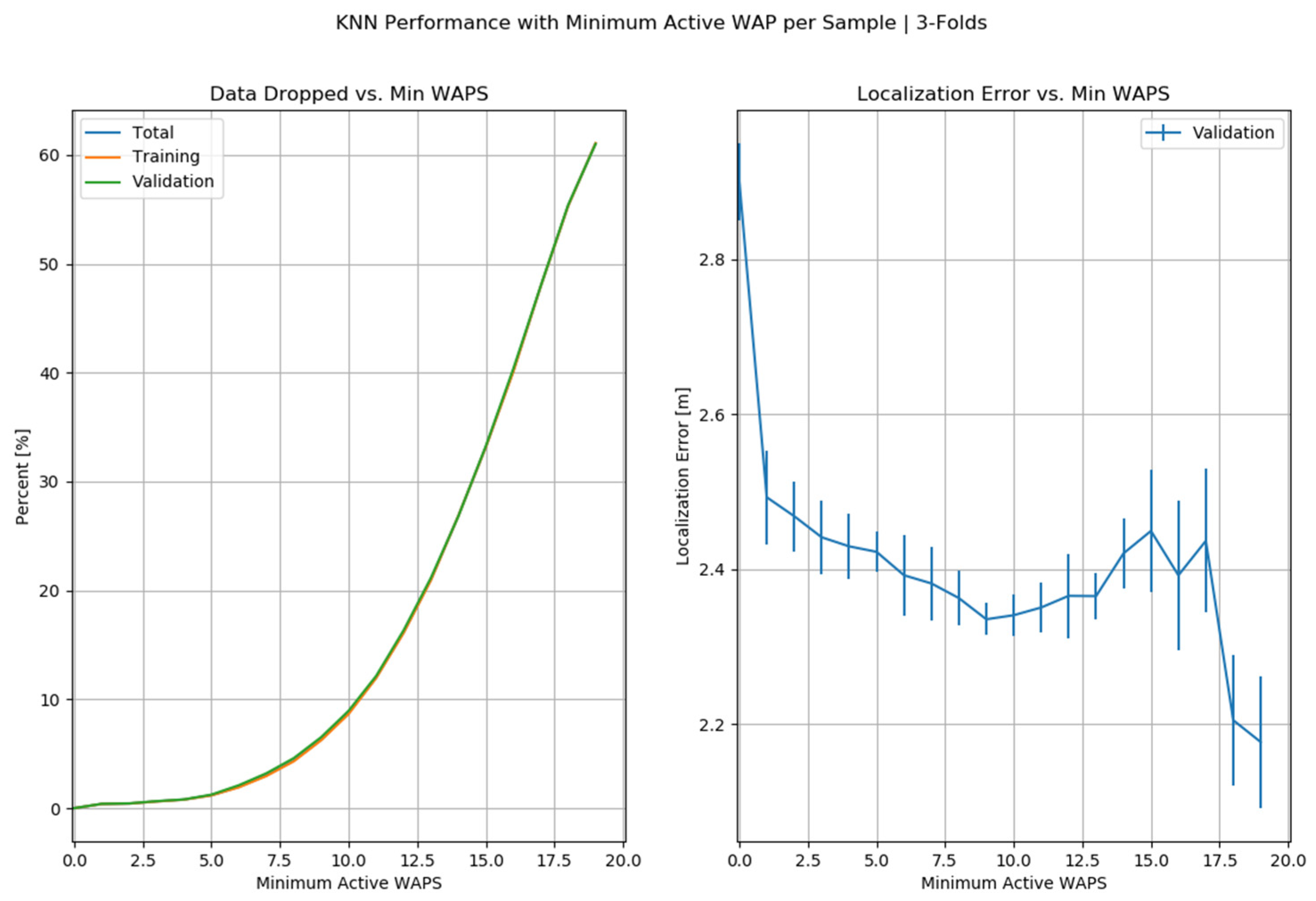
According to the predictions of machine-learning models, KNN has been considered the best regressor. Because it has minimum SE, BPE, and FPE, it has achieved 0.00% error rates, which shows the best performance of the KNN algorithm. Further, we have applied K-Folds cross-validation on KNN, as shown in Figure 17.

Figure 17.
K-Folds Cross-Validation at KNN.
KNN has shown good performance with an optimized error rate at threefold cross-validation, which can be seen in Figure 18.
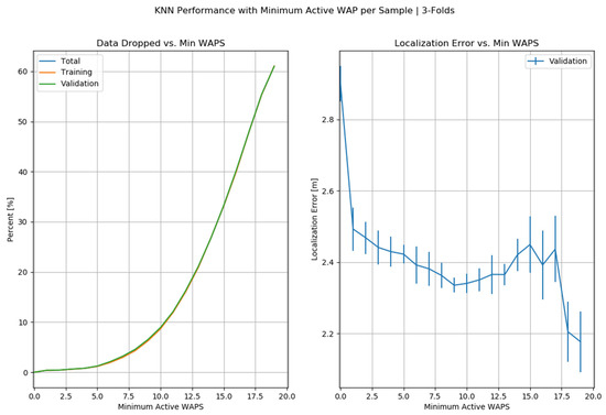
Figure 18.
K = 3 Cross-Validation in KNN.
4.5. Convolutional Neural Network
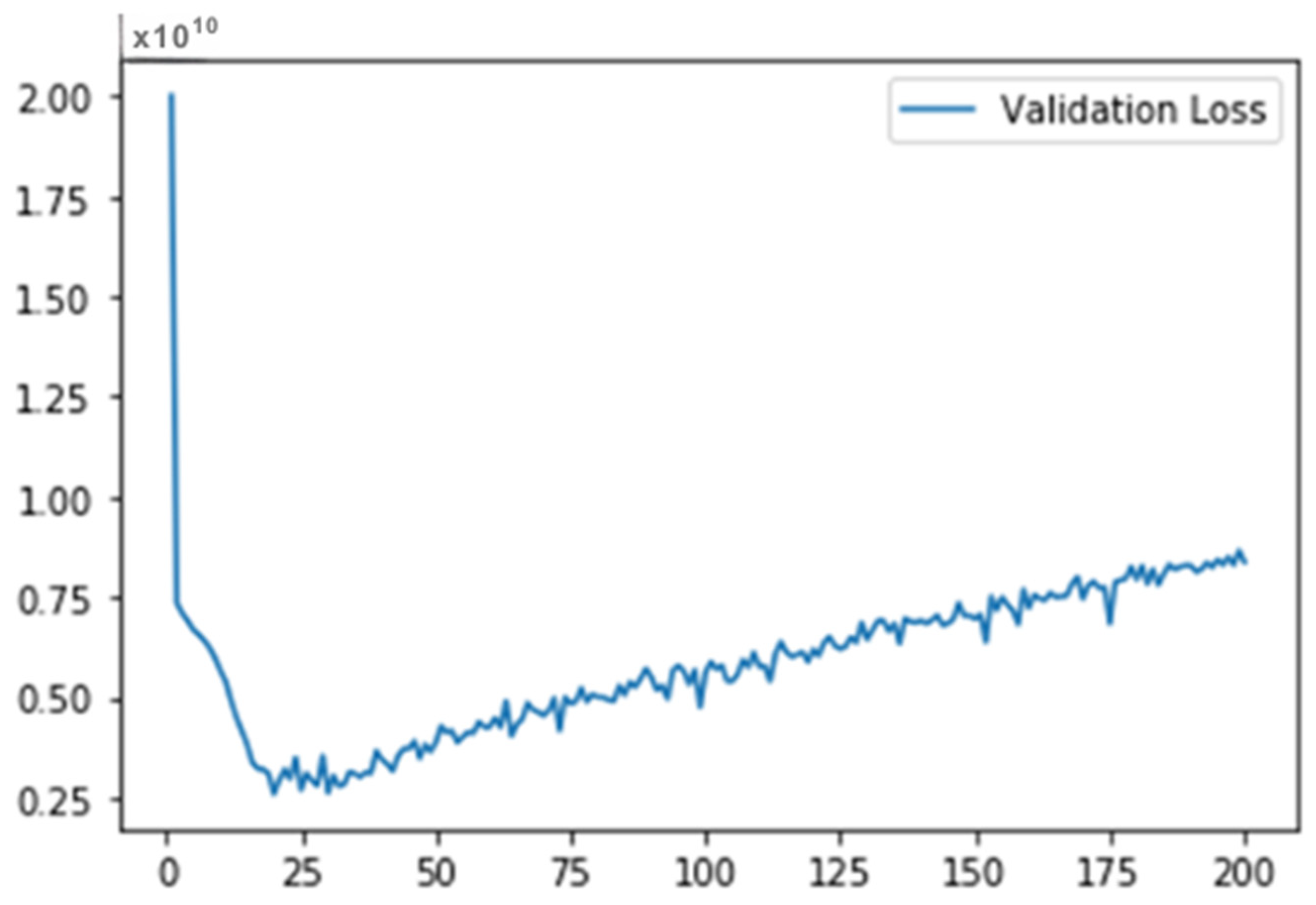
The two procedures discussed before, that is, convolutions and pooling can be considered feature extractors. Afterwards, we transmit this feature to the network, usually as a reshaped vector of one row. To validate the current research work, we have optimized the CNN model by using three optimizers. CNN has shown good performance. Figure 19 shows MSE loss during the Validation of Testing data by CNN-ADAM. Figure 20 shows the validation set performance of CNN with the ADAM optimizer, SGD optimizer, and RMSProp optimizer.

Figure 19.
MSE Loss during Validation of Testing Data by CNN-ADAM.
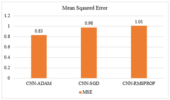
Figure 20.
Comparison of CNN Hyper-Tuned Models.
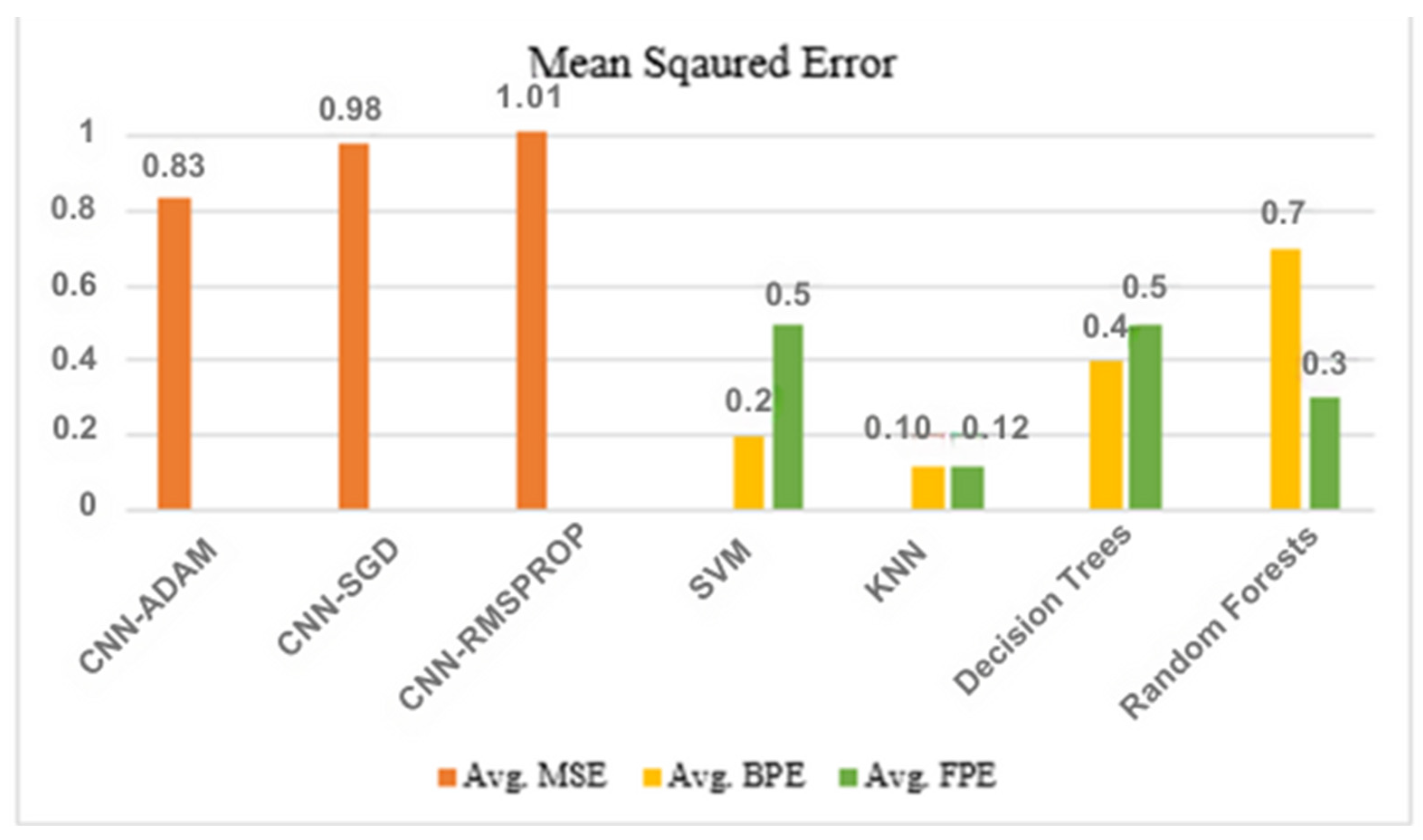
ADAM shows an MSE of 0.83, while SGD and RMSProp have shown MSEs of 0.98 and 1.010, respectively. The figure below shows the comparative analysis of the average mean squared error of the three hyper-tuned models of CNN.
4.6. Comparative Study
This study applied different Machine-learning models and Deep Learning Hyper-Tuned Models. All the models have shown promising results, among these models CNN-ADAM and KNN are the best models in terms of MSE, FPE, and BPE, respectively. Figure 21 shows the performance of each model in terms of metric evaluation.

Figure 21.
K-Folds Cross-Validation in KNN.
Five solutions were created for the UJIIndoorLoc indoor positioning dataset. The KNN model gave the lowest positional and localization errors, beating the baseline in the paper, in all except for the 95th and 100th percentiles. The building hit rate was 100%, and the floor hit rate, at 90.4%, was around 5% higher than the benchmark. The CNN-ADAM model had a slightly higher overall positional error as a mean squared error than the benchmark. Finally, the Random Forest model gave higher positional errors and a slightly lower building hit rate at 98.6%. Its floor hit rate, at 88%, still outperformed the baseline. Furthermore, research can be implemented on outdoor localization and positioning. It can be very beneficial in terms of predicting the localization and positional errors.
In comparing the results of this study with existing literature, the performance of the machine-learning models used for indoor localization can be evaluated. The Random Forest approach in my study has shown competitive accuracy, with Mean Coordinate Error (MCE) ranging from 1.28 to 19.19 m across different phone IDs. This places my results in line with or better than previous research, such as Wei and Akinci [16], which achieved 90% accuracy using an image-based method, and Tiku et al. [18], which achieved 85% to 95% accuracy using Support Vector Machines (SVMs) and deep neural networks (DNNs). Additionally, the K-Nearest Neighbors (KNN) method used in this study stands out, with an MCE ranging from 1.2 to 2.28 m, demonstrating accuracy levels comparable to or exceeding those of many referenced works. Furthermore, the use of Support Vector Machine (SVM) models in this study has shown promising results with MCE ranging from 34.63 to 58.37 m, placing my results within the range of other studies using SVMs.
Methodologically, this study aligns with prior literature in its use of machine-learning models like Random Forests, KNN, and SVMs for indoor localization. However, these results show significant improvements in accuracy, particularly with KNN outperforming other studies in terms of MCE, SE, Building % Error (BPE), and Floor % Error (FPE). This suggests that the current approach of optimizations has resulted in more accurate localization outcomes compared to several referenced works. Additionally, the visualization of the results using radio maps for each phone ID, like the approaches of other studies, allows for a clear comparison of predicted and actual locations, enhancing the transparency and understanding of my methodology and results.
5. Case Study
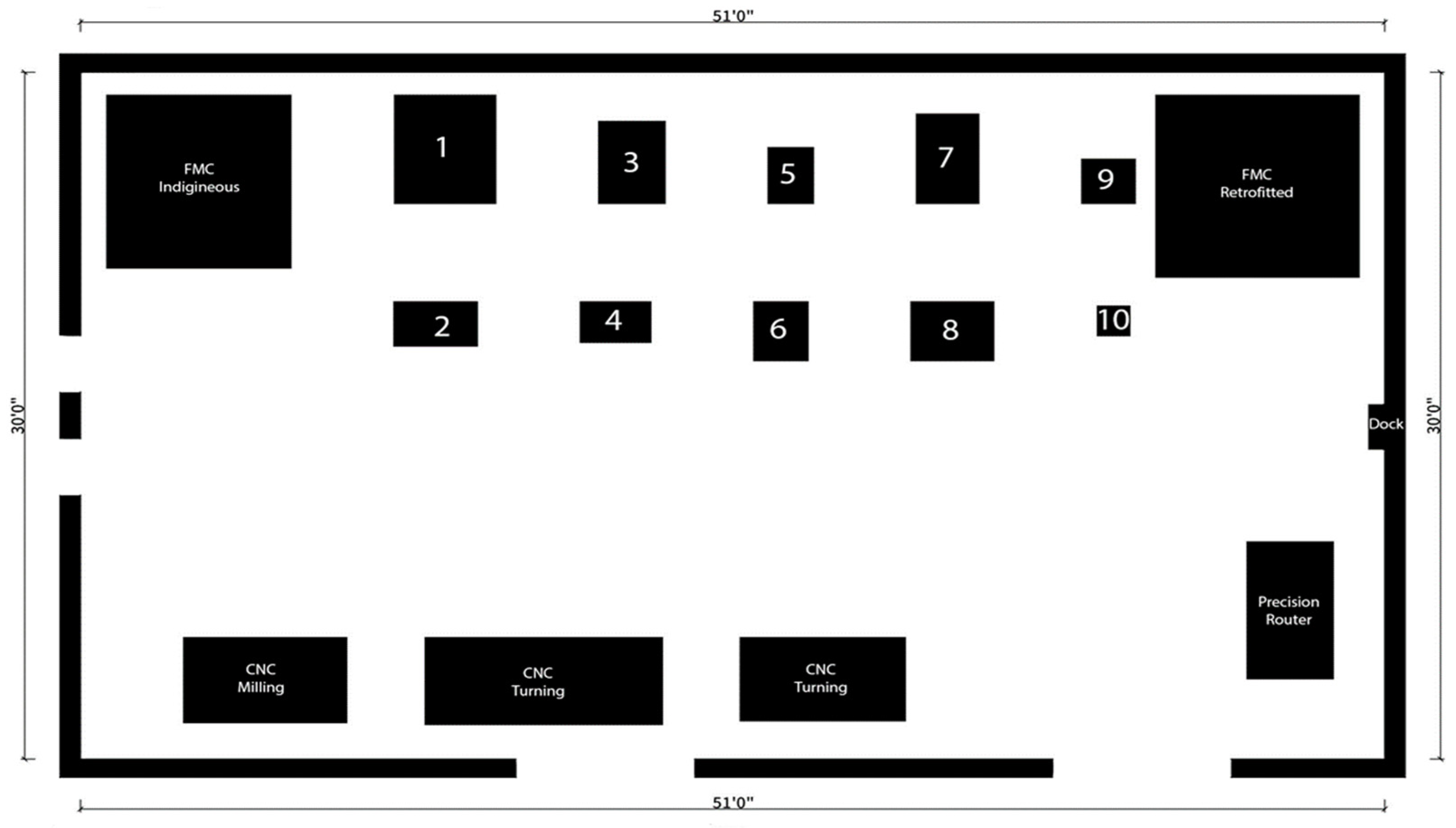
To demonstrate the application of the proposed localization and deep reinforcement learning techniques, a case study was developed using a collaborative robot (Co-Bot) in a laboratory environment. The lab is 51 × 30 feet in area. The lab was leveraged in this study due to its existing capabilities and flexible layout, which allowed the implementation of the proposed Digital Twin framework. While not originally designed exclusively for this research, the lab provided an optimal environment for experimentation due to its integration of IoT-enabled equipment and the spatial arrangement conducive to deploying Wi-Fi access points.
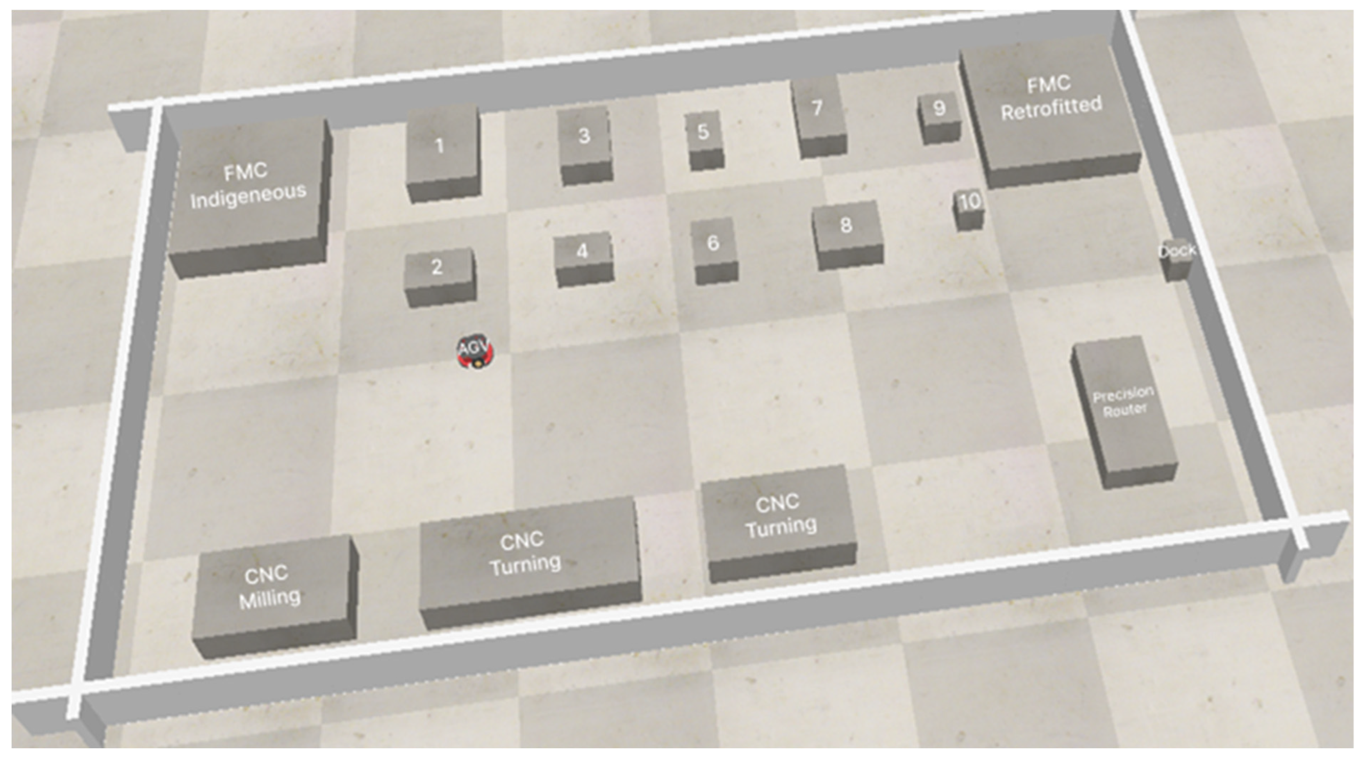
The Co-Bot has a LiDAR sensor, but for this experiment, it was disconnected, to verify the accuracy and application impact on the localization. The Digital twin is populated with the CAD models of all the static obstacles. As can be seen in Figure 22, the layout shows two Flexible Manufacturing Systems in the upper two corners. The selective laser jet, pneumatic jet, 3D scanner, coordinate measuring machine, and binder jet printer are located in between and are denoted as 1, 2, 3, etc. They act as static obstacles for the Co-Bot, while humans (technicians, researchers, etc.) act as dynamic obstacles.

Figure 22.
Layout of Advanced Manufacturing Processes Lab (Wi-Fi Localization Visualization through CO-Bot).
The front end of the Digital Twin offers two coordinate points for the Co-Bot. The first one is the starting point, and the second one is the endpoint. At the back end of the Digital Twin, the deep reinforcement learning algorithm is used. In addition to localization, a deep reinforcement learning (RL) agent was developed to generate optimal paths between destinations while avoiding collisions. The RL agent was trained in a simulation environment created from the Digital Twin layout. The agent learned to maximize rewards for reaching goals safely.
It calculates the trajectory based on starting and ending points. Moreover, the static and dynamic obstacles are incorporated in online mode, as it recalculates its trajectory. The DT is fed with data from the models.
Through the localization data from the learning models, the Digital Twin radio map was constructed. The map is showcased in Figure 23.
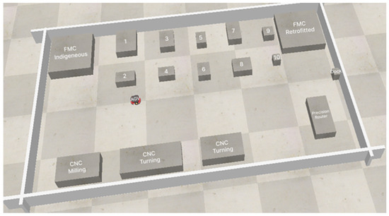
Figure 23.
Radio Map Generated through Digital Twin (Wi-Fi Localization Visualization through CO-Bot).
For the experiment, the Co-Bot was deployed in this lab environment and tasked with performing material handling jobs. For precise localization, Wi-Fi access points were installed throughout the lab as well and IOT sensors were mounted on all the equipment to act as obstacles for the Co-Bot while the mobile phones of the technicians and researchers were used to create dynamic obstacles. The system gathered Wi-Fi RSSI data which were fed to the trained deep CNN model for real-time position tracking.
Figure 24 shows the Co-Bot operating in the lab environment. The CNN model predicted the location coordinates within an average error of 1 m. This allowed the construction of an accurate Digital Twin of the lab with the Co-Bot’s current position.
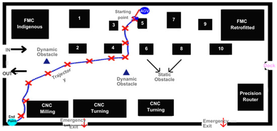
Figure 24.
Co-Bot Operating in the Lab.
This case study successfully demonstrated the integration of Wi-Fi fingerprinting, deep learning for localization, and deep RL for planning behaviors in Co-Bots. The techniques can be extended to other Automated Guided Vehicles in industrial environments to improve navigation accuracy and safety.
6. Conclusions
The study presents a novel framework for Flexible Manufacturing System (FMS). The framework combines Wi-Fi fingerprinting, deep learning for indoor localization, and Digital Twin technology. It is conducted to optimize real-time tracking in FMS. In modern factories, there is a widespread presence of Wi-Fi networks. This approach leverages this Wi-Fi presence and offers a cost-effective, dynamic, and scalable solution for creating Digital Twins of FMS environments.
The evaluation of the framework included several machine-learning models. Among the lot, KNN and CNN demonstrated exceptional accuracy. It achieved a mean coordinate error (MCE) between 1.2 and 2.28 m and a 100% building detection rate. The CNN-ADAM combination further highlighted the potential for deep learning for indoor localization. The CNN-ADAM combination had a mean squared error of 0.83. Additionally, deep reinforcement learning was used in conjunction with Automated Guided Vehicle (AGV). It enabled AGV to navigate and avoid obstacles with 100% success in a laboratory setting.
In comparison with the existing sensor-based Digital Twin, the Wi-Fi-based localization offers a more flexible and scalable solution. Future research could explore incorporating additional data sources. A lot of focus can be applied to testing the framework’s scalability in a larger manufacturing environment where everything is clustered. Finally, this framework advances to Industry 4.0. The advancement is through more efficient, data-driven manufacturing processes that contribute to greater productivity, cost savings, and competitiveness.
6.1. Future Work
Future studies could focus on expanding the proposed framework’s scalability and functionality to address more complex and diverse industrial scenarios. Testing this approach in larger, real-world manufacturing setups, where numerous machines, Automated Guided Vehicles (AGVs), and human operators interact simultaneously, would provide critical insights into its adaptability and robustness.
Additionally, integrating data from other advanced sources, such as LiDAR, RFID, and multi-modal sensors, could further enhance localization accuracy and provide richer, more nuanced operational insights.
Hybrid localization techniques that combine Wi-Fi fingerprinting with other technologies, such as vision-based localization or ultra-wideband (UWB) systems, also represent a promising area for future exploration. These techniques could offer more resilient solutions across diverse environments, particularly in challenging industrial layouts.
6.2. Limitations
The computational demands of integrating machine-learning models and real-time localization could restrict deployment in resource-constrained settings. Small and medium-sized enterprises may also find the initial setup costs for implementing IoT sensors, Wi-Fi access points, and Digital Twin platforms prohibitive.
Additionally, the framework has primarily been validated in controlled laboratory environments. This limited scope may not capture the full spectrum of challenges encountered in operational industrial contexts, necessitating further real-world testing.
By addressing these limitations and pursuing the outlined future research directions, the proposed framework has the potential to evolve into a more versatile, scalable, and impactful solution for advancing smart manufacturing systems.
Author Contributions
Conceptualization, A.U.; Software, A.U.; Validation, M.S.S.; Writing—original draft, A.U.; Writing—review & editing, M.Y. All authors have read and agreed to the published version of the manuscript.
Funding
This research received no external funding.
Data Availability Statement
Data are contained within the article.
Conflicts of Interest
The authors declare no conflict of interest.
Abbreviations
| Abbreviation | Full Name | Description |
| AI | Artificial Intelligence | A branch of computer science dealing with intelligent agents |
| DT | Digital Twin | A virtual representation of a physical asset or system |
| FMS | Flexible Manufacturing System | A production system capable of handling a variety of products |
| IoT | Internet of Things | A network of physical devices embedded with sensors, software, and other technologies for data collection and communication |
| CNN | Convolutional Neural Network | A type of artificial neural network used for image recognition and classification |
| KNN | K-Nearest Neighbors | A machine-learning algorithm for classification and regression tasks |
| SVM | Support Vector Machine | A machine-learning algorithm for classification and regression tasks |
| RF | Random Forest | A machine-learning algorithm consisting of an ensemble of decision trees |
| DT | Decision Tree | A machine-learning algorithm for classification tasks represented as a tree structure |
| RSS | Received Signal Strength | A measure of the power level of a received radio signal |
| CSI | Channel State Information | Information about a communication channel, often used for indoor positioning |
| RNN | Recurrent Neural Network | A type of artificial neural network that can process sequential data |
| LSTM | Long Short-Term Memory | A type of recurrent neural network capable of learning long-term dependencies |
| FPGA | Field Programmable Gate Array | An integrated circuit whose internal connections can be programmed for specific functionality |
| RGBD | Red, Green, Blue, Depth | A type of camera that captures color and depth information |
| BIM | Building Information Modeling | A digital representation of a building, including its geometry and functional properties |
| RMSPROP | Root Mean Square Propagation | An optimization algorithm used for training neural networks |
| SGD | Stochastic Gradient Descent | An optimization algorithm used for training neural networks |
| ADAM | Adaptive Moment Estimation | An optimization algorithm used for training neural networks |
| MSE | Mean Squared Error | A measure of the average squared difference between predicted and actual values |
| MCE | Mean Coordinate Error | A measure of the average distance between predicted and actual locations |
| SE | Standard Error | A measure of the variability of a sample statistic |
| BPE | Building Percentage Error | The percentage of localization errors where the wrong building is identified |
| FPE | Floor Percentage Error | The percentage of localization errors where the wrong floor within a building is identified |
| AGV | Automated Guided Vehicle | A self-propelled mobile robot used for transporting materials within a manufacturing facility |
| LiDAR | Light Detection and Ranging | A remote sensing method that uses light to measure distance |
| CAD | Computer-Aided Design | The use of computer software to create and modify designs |
| RL | Reinforcement Learning | A type of machine-learning where an agent learns through trial and error in an interactive environment |
| RSSI | Received Signal Strength Indicator | A measurement of the power level of a received radio signal (alternative definition) |
| dBm | Decibel-milliwatts | A unit of power measurement |
| CSV | Comma-Separated Values | A file format used to store tabular data |
| DCNN | Deep Convolutional Neural Network | A convolutional neural network with multiple layers |
| AoA | Angle of Arrival | The direction from which a radio signal arrives |
| ELM | Extreme Learning Machine | A type of artificial neural network with randomly chosen hidden layer weights |
| CCR-ELM | Class-specific Cost Regulation Extreme Learning Machine | A variant of ELM with a cost function that considers class imbalance |
| DFL | Device-Free Localization | Localization techniques that do not require users to carry any dedicated devices |
| 6DoF | 6 Degrees of Freedom | The ability of an object to move freely in three-dimensional space |
| RF | Radiofrequency | A range of electromagnetic frequencies used for wireless communication |
| R-CNN | Region-based Convolutional Neural Networks | A type of convolutional neural network used for object detection |
| SAE | Stacked Auto-Encoder | A type of neural network architecture used for dimensionality reduction |
| WiDeep | Wi-Fi-based Deep Learning Model | A type of deep learning model used for indoor localization utilizing Wi-Fi signals |
| CSI | Channel State Information (repeated entry) | Information about a communication channel, often used for indoor positioning |
| MIMO | Multiple-Input Multiple-Output | A technique used in wireless communication systems to transmit and receive multiple data streams simultaneously |
| MLP | Multi-Layer Perceptron | A type of artificial neural network with multiple layers of neurons |
References
- Árvai, L. Convolutional neural network-based activity monitoring for indoor localization. Pollack Period. 2021, 16, 7–12. [Google Scholar] [CrossRef]
- Zhao, B.; Zhu, D.; Xi, T.; Jia, C.; Jiang, S.; Wang, S. Convolutional neural network and dual-factor enhanced variational Bayes adaptive Kalman filter based indoor localization with Wi-Fi. Comput. Netw. 2019, 162, 106864. [Google Scholar] [CrossRef]
- Mittal, A.; Tiku, S.; Pasricha, S. Adapting convolutional neural networks for indoor localization with smart mobile devices. In Proceedings of the ACM Great Lakes Symposium on VLSI, GLSVLSI, Chicago, IL, USA, 23–25 May 2018; pp. 117–122. [Google Scholar] [CrossRef]
- Song, X.; Fan, X.; Xiang, C.; Ye, Q.; Liu, L.; Wang, Z.; He, X.; Yang, N.; Fang, G. A Novel Convolutional Neural Network Based Indoor Localization Framework with WiFi Fingerprinting. IEEE Access 2019, 7, 110698–110709. [Google Scholar] [CrossRef]
- Bregar, K.; Mohorcic, M. Improving Indoor Localization Using Convolutional Neural Networks on Computationally Restricted Devices. IEEE Access 2018, 6, 17429–17441. [Google Scholar] [CrossRef]
- Chen, K.M.; Chang, R.Y.; Liu, S.J. Interpreting Convolutional Neural Networks for Device-Free Wi-Fi Fingerprinting Indoor Localization via Information Visualization. IEEE Access 2019, 7, 172156–172166. [Google Scholar] [CrossRef]
- Chen, Z.; Alhajri, M.I.; Wu, M.; Ali, N.T.; Shubair, R.M. A Novel Real-Time Deep Learning Approach for Indoor Localization Based on RF Environment Identification. IEEE Sens. Lett. 2020, 4, 6–9. [Google Scholar] [CrossRef]
- Zhang, G.; Wang, P.; Chen, H.; Zhang, L. Wireless Indoor Localization Using Convolutional Neural Network and Gaussian Process Regression. Sensors 2019, 19, 2508. [Google Scholar] [CrossRef] [PubMed]
- Njima, W.; Njima, W.; Zayani, R.; Terre, M.; Bouallegue, R. Deep cnn for indoor localization in iot-sensor systems. Sensors 2019, 19, 3127. [Google Scholar] [CrossRef] [PubMed]
- Liu, Z.; Dai, B.; Wan, X.; Li, X. Hybrid wireless fingerprint indoor localization method based on a convolutional neural network. Sensors 2019, 19, 4597. [Google Scholar] [CrossRef]
- Ashraf, I.; Hur, S.; Park, S.; Park, Y. DeepLocate: Smartphone based indoor localization with a deep neural network ensemble classifier. Sensors 2020, 20, 133. [Google Scholar] [CrossRef] [PubMed]
- Koike-Akino, T.; Wang, P.; Pajovic, M.; Sun, H.; Orlik, P.V. Fingerprinting-Based Indoor Localization with Commercial MMWave WiFi: A Deep Learning Approach. IEEE Access 2020, 8, 84879–84892. [Google Scholar] [CrossRef]
- Jang, H.J.; Shin, J.M.; Choi, L. Geomagnetic field based indoor localization using recurrent neural networks. In Proceedings of the 2017 IEEE Global Communications Conference, GLOBECOM 2017—Proceedings, Singapore, 4–8 December 2017; Volume 2018, pp. 1–6. [Google Scholar] [CrossRef]
- Kim, K.S.; Lee, S.; Huang, K. A scalable deep neural network architecture for multi-building and multi-floor indoor localization based on Wi-Fi fingerprinting. Big Data Anal. 2018, 3, 4. [Google Scholar] [CrossRef]
- Liu, C.; Wang, C.; Luo, J. Large-Scale Deep Learning Framework on FPGA for Fingerprint-Based Indoor Localization. IEEE Access 2020, 8, 65609–65617. [Google Scholar] [CrossRef]
- Wei, Y.; Akinci, B. A vision and learning-based indoor localization and semantic mapping framework for facility operations and management. Autom. Constr. 2019, 107, 102915. [Google Scholar] [CrossRef]
- Zhong, Z.; Tang, Z.; Li, X.; Yuan, T.; Yang, Y.; Wei, M.; Zhang, Y.; Sheng, R.; Grant, N.; Ling, C.; et al. XJTLUIndoorLoc: A New Fingerprinting Database for Indoor Localization and Trajectory Estimation Based on Wi-Fi RSS and Geomagnetic Field. In Proceedings of the 2018 Sixth International Symposium on Computing and Networking Workshops (CANDARW), Takayama, Japan, 27–30 November 2018. [Google Scholar]
- Tiku, S.; Kale, P.; Pasricha, S. QuickLoc: Adaptive Deep-Learning for Fast Indoor Localization with Mobile Devices. ACM Trans. Cyber-Phys. Syst. 2021, 5, 1–30. [Google Scholar] [CrossRef]
- Tiku, S.; Pasricha, S. Overcoming security vulnerabilities in deep learning-based indoor localization frameworks on mobile devices. ACM Trans. Embed. Comput. Syst. 2019, 18, 1–24. [Google Scholar] [CrossRef]
- Wang, F.; Feng, J.; Zhao, Y.; Zhang, X.; Zhang, S.; Han, J. Joint activity recognition and indoor localization with WiFi fingerprints. IEEE Access 2019, 7, 80058–80068. [Google Scholar] [CrossRef]
- Lin, W.Y.; Huang, C.C.; Duc, N.T.; Manh, H.N. Wi-Fi Indoor Localization based on Multi-Task Deep Learning. In Proceedings of the International Conference on Digital Signal Processing, DSP, Shanghai, China, 19–21 November 2018; Volume 2018, pp. 1–5. [Google Scholar] [CrossRef]
- Chenning, L.; Ting, Y.; Qian, Z.; Haowei, X. Object-based Indoor Localization using Region-based Convolutional Neural Networks. In Proceedings of the 2018 IEEE International Conference on Signal Processing, Communications and Computing, ICSPCC 2018, Qingdao, China, 14–16 September 2018; pp. 1–6. [Google Scholar] [CrossRef]
- Abbas, M.; Elhamshary, M.; Rizk, H.; Torki, M.; Youssef, M. WiDeep: WiFi-based accurate and robust indoor localization system using deep learning. In Proceedings of the 2019 IEEE International Conference on Pervasive Computing and Communications, PerCom 2019, Kyoto, Japan, 11–15 March 2019; pp. 1–10. [Google Scholar] [CrossRef]
- Zhou, B.; Yang, J.; Li, Q. Smartphone-based activity recognition for indoor localization using a convolutional neural network. Sensors 2019, 19, 621. [Google Scholar] [CrossRef]
- Wang, X.; Wang, X.; Mao, S. Deep Convolutional Neural Networks for Indoor Localization with CSI Images. IEEE Trans. Netw. Sci. Eng. 2020, 7, 316–327. [Google Scholar] [CrossRef]
- Qi, Q.; Tao, F. Digital Twin and Big Data Towards Smart Manufacturing and Industry 4.0: 360 Degree Comparison. IEEE Access 2018, 6, 3585–3593. [Google Scholar] [CrossRef]
- Tao, F.; Cheng, J.; Qi, Q.; Zhang, M.; Zhang, H.; Sui, F. Digital twin-driven product design, manufacturing and service with big data. Int. J. Adv. Manuf. Technol. 2018, 94, 3563–3576. [Google Scholar] [CrossRef]
- Mourtzis, D.; Vlachou, E.; Milas, N. Industrial Big Data as a Result of IoT Adoption in Manufacturing. Procedia CIRP 2016, 55, 290–295. [Google Scholar] [CrossRef]
- Lee, J.; Bagheri, B.; Kao, H.A. A Cyber-Physical Systems architecture for Industry 4.0-based manufacturing systems. Manuf. Lett. 2015, 3, 18–23. [Google Scholar] [CrossRef]
- Fan, Y.; Yang, J.; Chen, J.; Hu, P.; Wang, X.; Xu, J.; Zhou, B. A digital-twin visualized architecture for Flexible Manufacturing System. J. Manuf. Syst. 2021, 60, 176–201. [Google Scholar] [CrossRef]
- Zhang, C.; Xu, W.; Liu, J.; Liu, Z.; Zhou, Z.; Pham, D.T. Digital twin-enabled reconfigurable modeling for smart manufacturing systems. Int. J. Comput. Integr. Manuf. 2021, 34, 709–733. [Google Scholar] [CrossRef]
- Negri, E.; Berardi, S.; Fumagalli, L.; Macchi, M. MES-integrated digital twin frameworks. J. Manuf. Syst. 2020, 56, 58–71. [Google Scholar] [CrossRef]
- Samir, K.; Maffei, A.; Onori, M.A. Real-Time asset tracking; a starting point for digital twin implementation in manufacturing. Procedia CIRP 2019, 81, 719–723. [Google Scholar] [CrossRef]
- Zhang, J.; Xiao, W.; Li, Y. Data and Knowledge Twin Driven Integration for Large-Scale Device-Free Localization. IEEE Internet Things J. 2021, 8, 320–331. [Google Scholar] [CrossRef]
- Park, S.; Kim, D.H.; You, C. Fi-Vi: Large-Area Indoor Localization Scheme Combining ML/DL-Based Wireless Fingerprinting and Visual Positioning. IEEE Access 2022, 10, 127094–127116. [Google Scholar] [CrossRef]
- Shu, M.; Chen, G.; Zhang, Z. 3D Point Cloud-Based Indoor Mobile Robot in 6-DoF Pose Localization Using a Wi-Fi-Aided Localization System. IEEE Access 2021, 9, 38636–38648. [Google Scholar] [CrossRef]
- Hu, X.; Assaad, R.H. A BIM-enabled digital twin framework for real-time indoor environment monitoring and visualization by integrating autonomous robotics, LiDAR-based 3D mobile mapping, IoT sensing, and indoor positioning technologies. J. Build. Eng. 2024, 86, 108901. [Google Scholar] [CrossRef]
- Pauwels, P.; de Koning, R.; Hendrikx, B.; Torta, E. Live semantic data from building digital twins for robot navigation: Overview of data transfer methods. Adv. Eng. Inform. 2023, 56, 101959. [Google Scholar] [CrossRef]
- Wong, M.O.; Lee, S. Indoor navigation and information sharing for collaborative fire emergency response with BIM and multi-user networking. Autom. Constr. 2023, 148, 104781. [Google Scholar] [CrossRef]
- Abdelrahman, M.M.; Chong, A.; Miller, C. Personal thermal comfort models using digital twins: Preference prediction with BIM-extracted spatial–temporal proximity data from Build2Vec. Build. Environ. 2022, 207, 108532. [Google Scholar] [CrossRef]
- Morais, J.; Alkhateeb, A. Localization in Digital Twin MIMO Networks: A Case for Massive Fingerprinting. arXiv 2024, arXiv:2403.09614. Available online: http://arxiv.org/abs/2403.09614 (accessed on 10 July 2024).
- Karakusak, M.Z.; Kivrak, H.; Watson, S.; Ozdemir, M.K. Cyber-WISE: A Cyber-Physical Deep Wireless Indoor Positioning System and Digital Twin Approach. Sensors 2023, 23, 9903. [Google Scholar] [CrossRef]
- Qian, C.; Liu, X.; Ripley, C.; Qian, M.; Liang, F.; Yu, W. Digital Twin—Cyber Replica of Physical Things: Architecture, Applications and Future Research Directions. Future Internet 2022, 14, 64. [Google Scholar] [CrossRef]
- Zhuang, C.; Miao, T.; Liu, J.; Xiong, H. The connotation of digital twin, and the construction and application method of shop-floor digital twin. Robot. Comput. Integr. Manuf. 2021, 68, 102075. [Google Scholar] [CrossRef]
- Xu, R.; Park, C.W.; Khan, S.; Jin, W.; Moe, S.J.S.; Kim, D.H. Optimized Task Scheduling and Virtual Object Management Based on Digital Twin for Distributed Edge Computing Networks. IEEE Access 2023, 11, 114790–114810. [Google Scholar] [CrossRef]
- Manocha, A.; Sood, S.K.; Bhatia, M. IoT-digital twin-inspired smart irrigation approach for optimal water utilization. Sustain. Comput. Inform. Syst. 2024, 41, 100947. [Google Scholar] [CrossRef]
- Wang, S.; Zhang, J.; Wang, P.; Law, J.; Calinescu, R.; Mihaylova, L. A deep learning-enhanced Digital Twin framework for improving safety and reliability in human–robot collaborative manufacturing. Robot. Comput. Integr. Manuf. 2024, 85, 102608. [Google Scholar] [CrossRef]
- Akhtar, M.S.; Feng, T. IoT Based Indoor and Outdoor Localization Framework with WI-FI Fingerprinting Based on Scalable Resnet Models. Rev. Comput. Eng. Stud. 2022, 9, 53–66. [Google Scholar] [CrossRef]
- Ullah, A.; Younas, M. Development and Application of Digital Twin Control in Flexible Manufacturing Systems. J. Manuf. Mater. Process. 2024, 8, 214. [Google Scholar] [CrossRef]


Disclaimer/Publisher’s Note: The statements, opinions and data contained in all publications are solely those of the individual author(s) and contributor(s) and not of MDPI and/or the editor(s). MDPI and/or the editor(s) disclaim responsibility for any injury to people or property resulting from any ideas, methods, instructions or products referred to in the content. |
© 2025 by the authors. Licensee MDPI, Basel, Switzerland. This article is an open access article distributed under the terms and conditions of the Creative Commons Attribution (CC BY) license (https://creativecommons.org/licenses/by/4.0/).