Numerical Investigation and Experimental Verification of Vibration Behavior for a Beam with Cantilever-Hertzian Contact Boundary Conditions

Abstract

The simple spring structure, with detachable electrical contacts, is a very suitable solution for many applications, such as electromechanical relays and connectors. However, they are prone to exhibit instantaneous interruption faults under mechanical vibration environments. In this paper, the governing equations of the modal analysis of a beam with cantilever-Hertzian contact boundary conditions are presented. Then, the time domain analysis method and frequency domain analysis method for solving the forced vibration response are described explicitly. Next, the effect of the axial force on the modal frequency of a detailed model sourced from the practical relay is investigated by using commercial ANSYS Workbench 2021R1 software. Afterward, the harmonic response of the beam is numerically solved individually by using the transient analysis model and the harmonic analysis model in ANSYS Workbench 2021R1 software. Then, the influences of the damping coefficient and excited frequency on the contact force response are investigated. The experimental results of transient displacement and contact resistance of the beam structure agree well with the simulation outcomes. It is proven that there is a linear relationship between the stiffness coefficient and the mass coefficient, which are used for characterizing the damping of the structures in the time domain method and frequency domain methods.

1. Introduction

The simple spring structure plays a major role in electromechanical relays and connectors for carrying mechanical force load and electrical current load at the same time [1,2]. As shown in Figure 1, it consists of a cantilevered beam riveted with a cambered electrode and a static electrode. The prestressed configuration could provide the normally closed contact pair for current passing; meanwhile, the detachable contact is designed for current interruption. Undoubtedly, such kinds of structures are more sensitive to a mechanical vibration environment. Once the exerted vibration strength reaches the threshold value, substantial variations in contact force and associated contact resistance inevitably occur. Field data has shown the instantaneous break-off phenomena that occur in the interconnection extremely influence the signal integrity or power transmission reliability of the electrical circuit [3,4].

Many efforts have been devoted to investigating the vibration behaviors of spring structures. Рoйзен [5] was interested in the vibrations of a beam for modeling electromechanical relay dynamics, whereby the boundary conditions of the beam were taken as the fixed end and hinged support. Chambega [6] proposed an analytical approach to study natural frequency by modeling it as a simple linear single degree-of-freedom (DOF) system. Ren and Zhai [7] simplified the beam with Hertzian contact into a two-DOF system by introducing the equivalent contact rigidity, and then the non-linear normal modes were observed. The non-linear vibration behavior of beams with non-linear boundary conditions has been investigated far less using the perturbation approach [8], harmonic balance method [9], and the multiple scales method [10], but the initial prestressed status of the beam can only be ignored by using such semi-analytical approaches.

With the availability of advanced computing facilities and finite element codes, the feasibility of conducting virtual vibration tests via finite element simulation may be realized. The simulations of vibration behaviors of such structures have been examined previously by a number of authors [11,12,13,14,15]. Xie et al. [11] developed a two-dimensional finite element model of the contact pair to determine the relative motion mode and the resonant frequency of the contact pair using modal analysis. Rezaei et al. [12,13] established a co-relationship between Young’s modulus of the materials and the modal frequency of beams with rectangular beam structures. The focus in these works was mainly on normal modes and associated harmonic response [14,15], but the authors themselves suggested that some aspects should be studied deeply.

In addition, Almeida et al. [16] investigated the aeroelastic stability boundary of flutter in aircraft composite panels, revealing that axial prestress significantly influences the natural frequency of these panels. Both Tchomeni [17] and Tomović [18] proved that time domain dynamic equations are more suitable for solving the vibration response of structures with nonlinear boundary conditions. However, the time domain method is characterized by lengthy computation times and limited applicability to addressing fixed frequency vibration issues. Wuk et al. [19] recommended the utilization of the modal superposition method to calculate the harmonic response, with subsequent application of the time domain method for adjustments. Admittedly, the contact force response and associated calculation accuracy are closely dependent on the set damping coefficients. Unfortunately, relatively little is known about the selection method of damping coefficients for numerical simulation. Such a status quo causes the calculation results obtained by finite element simulation to be questioned to a certain extent.

This paper is organized as follows. First, in Section 2, the dynamics of a linear beam with cantilever-Hertzian contact boundary conditions are described. Besides, a numerical analysis for the forced vibration response is made by using the frequency domain method and time domain method individually. Finite element simulation for a detailed beam structure example is described in Section 3 by calculating the normal modes and the contact force responses with different damping coefficients. Then, in Section 4, experimental tests have been carried out to validate the simulation model, and the two kinds of harmonic response simulation method are compared. Finally, the conclusion of the research is presented in Section 5.

2. Theoretical Background

2.1. Governing Equations for Modal Analysis

As illustrated in Figure 2, a uniform homogeneous beam with constant cross-section is cantilevered at the left end. At the right end of the beam (x = L), a cumbered electrode with curvature radius R is attached. The electrode is in contact with a flat electrode. The contact force between the two electrodes is realized by adjusting the vertical offset s of the flat electrode. The vertical overtravel s produces the deflection y(L) of the beam at the contact position and the elastic deformation of the electrode surface δ. It is written by:

$$s=y(L)+\delta$$

(1)

The non-linear vibration problem for this system has a governing equation given by:

$$EI{\displaystyle \frac{{\partial }^{4}y(x,t)}{\partial x^4}}+\rho A{\displaystyle \frac{{\partial }^{2}y(x,t)}{\partial t^2}}-N{\displaystyle \frac{{\partial }^{2}y(x,t)}{\partial x^2}}=p(x,t)$$

(2)

with boundary conditions:

$$y(x,t)=0, \mathrm{at} x=0$$

(3)

$$y^{\prime }(x,t)=0, \mathrm{at} x=0$$

(4)

$$EI{y}^{″}(x,t)=0, \mathrm{at} x=L$$

(5)

$$EI{y}^{‴}(x,t)-k_{j}y(x,t)=0, \mathrm{at} x=L$$

(6)

The boundary condition given by Equation (6) is the force balance between the shear force in the beam and the contact force associated with two electrodes. According to the classical Hertz contact theory [20], the relationship between the load force P and the elastic deformation δ can be expressed by:

$$P={\displaystyle \frac{4E^{*}}{3}}{R}^{1/2}{\delta }^{3/2}$$

(7)

where $E^{*}={\left({\displaystyle \frac{1-{\sigma }_1^2}{E_1}}+{\displaystyle \frac{1-{\sigma }_2^2}{E_2}}\right)}^{-1}$ is the equivalent elastic modulus.

In Equation (6), the equivalent contact stiffness k_j is introduced to describe the Hertzian contact force with the known elastic deformation. It is defined by:

$$k_j={\displaystyle \frac{\mathrm{d}P}{\mathrm{d}\delta }}=2E^{*}{R}^{1/2}{\delta }^{1/2}={(6E^{*2}RP)}^{1/3}$$

(8)

Note that the equivalent contact stiffness is closely dependent on the normal contact force.

Meanwhile, the axial force N is governed by:

$$N={\displaystyle \frac{3EIy(L)}{L^3\sin (\frac{3y(L)}{2L})}}$$

(9)

Assuming that $y(x,t)=Q(x)T(t)$, in which Q(x) is the mode function, T(t) is the time function, the general solution of Q(x) is given by:

$$Q(x)=C_1\sin (s_{1}x)+C_2\cos (s_{1}x)+C_3\sinh (s_{2}x)+C_4\cosh (s_{2}x)$$

(10)

in which ${\alpha }^4={\omega }^2{\displaystyle \frac{\rho A}{EI}}$, $\beta =\sqrt{{\displaystyle \frac{N}{EI}}}$ and:

$$\left\{\begin{array}{l}{s}_1=\sqrt{-{\displaystyle \frac{{\beta }^2}{2}}+\sqrt{{\displaystyle \frac{{\beta }^4}{4}}+{\alpha }^4}}\\ s_2=\sqrt{{\displaystyle \frac{{\beta }^2}{2}}+\sqrt{{\displaystyle \frac{{\beta }^4}{4}}+{\alpha }^4}}\end{array}\right.$$

(11)

Substituting Equations (3)–(6) into Equation (10), the solutions of s₁ and s₂ should satisfy:

$$\begin{array}{l}{s}_1^4+s_2^4+2s_1^2{s}_2^2·\cos (s_{1}L)·\cosh (s_{2}L)-s_1{s}_2(s_1^2-s_2^2)·\sin (s_{1}L)\sinh (s_{2}L)\\ ={\displaystyle \frac{k_j}{EI}}[({\displaystyle \frac{s_1^2}{s_2}}+s_2)·\cos (s_{1}L)·\sinh (s_{2}L)-({\displaystyle \frac{s_2^2}{s_1}}+s_1)·\sin (s_{1}L)·\cosh (s_{2}L)]\end{array}$$

(12)

The natural frequency of the beam is influenced by the stiffness of the contact zone and the axial force through Equation (12). Meanwhile, Almeida [16] concluded that an increase in axial pressure would reduce the natural frequency of the system.

The basic theoretical framework of a beam with cantilever-Hertzian contact boundary conditions is shaped by above governing equations for addressing the vibration behavior. It reveals that a reduction in the length of the free end or an increase in overtravel results in an enhancement of both the stiffness of the contact area and the axial force, and the associated natural frequency. The associated quantitative solutions are obtained by using the commercial software ANSYS Workbench 2021R1, which makes the calculation results easy to compare with the experimental results.

2.2. Harmonic Response for Forced Vibration in Time Domain

Two optional methods could be used for analyzing harmonic vibrations of flexible beam structures. One is the time domain analysis method, and the other one is the frequency domain analysis method. The time domain analysis method utilizes the transient kinematic equation as the mathematical model for vibration calculation. It is governed by:

$$[\mathrm{M}]\left\{\ddot{y}\right\}+[\mathrm{C}]\left\{\dot{y}\right\}+[\mathrm{K}]\left\{y\right\}=\{P(t)\}$$

(13)

where [M], [C], and [K] denote the mass matrix, the damping matrix, and the stiffness matrix of the flexible beam structure, respectively. The function P(t) denotes a variable load vector. [C] is also called the Rayleigh damping model, written as:

$$[\mathrm{C}]=\alpha [\mathrm{M}]+\beta [\mathrm{K}]$$

(14)

in which α is the mass coefficient and β is the stiffness coefficient. In many practical structural problems, α is taken as zero. Mass damping may be ignored. The stiffness coefficient β should satisfy:

$$\beta ={\displaystyle \frac{2{\xi }_i}{{\omega }_i}}$$

(15)

in which ω_i is the ith natural frequency and ξ_i is the corresponding constant.

For a beam with cantilever-Hertzian contact boundary conditions, the stiffness matrix [K] and the damping matrix [C] are closely dependent on time. So, the time domain analysis method for harmonic response of such beam demands the update the stiffness matrix [K] and the damping matrix [C] in each time step. After the stiffness matrix and damping matrix are updated at each time step, the displacement response of the system is recalculated, resulting in an updated contact force.

2.3. Harmonic Response for Forced Vibration in Frequency Domain

The solving method of the forced vibration response in the frequency domain is the classical modal superposition method, which takes the displacement response as a linear combination of involved characteristic modes of structures. The displacement response y(t) is expressed as:

$$y(t)\approx {\displaystyle \sum _{i=1}^n{a}_i(t){\varphi }_i} \mathrm{or} y=\Phi a$$

(16)

where a_i(t) is the modal amplitude and ϕ_i is the modal shape.

The solution of the eigenvalue problem:

$$(-{\omega }^2\mathrm{M}+\mathrm{K})\Phi =0,\Phi \ne 0$$

(17)

gives the natural frequencies of vibration and the modal shape matrix Φ.

The matrix Φ has orthogonality properties with mass and stiffness matrices. These properties are expressed as:

$${\Phi }_{\mathrm{N}}^{\mathrm{T}}\mathrm{M}{\Phi }_{\mathrm{N}}=\mathrm{E}$$

(18)

and:

$${\Phi }_{\mathrm{N}}^{\mathrm{T}}\mathrm{K}{\Phi }_{\mathrm{N}}=\Lambda$$

(19)

The matrix Φ_N denotes the result of the regularization process applied to the matrix Φ. The matrix E is the unit matrix, with elements that possess dimensions of mass, while Λ is a diagonal matrix constructed from the squares of the natural frequencies.

Equation (16) is substituted into Equation (13) and multiplied by Φ_N, yielding:

$${\Phi }_{\mathrm{N}}^{\mathrm{T}}\mathrm{M}{\Phi }_{\mathrm{N}}\ddot{a}+{\Phi }_{\mathrm{N}}^{\mathrm{T}}\mathrm{C}{\Phi }_{\mathrm{N}}\dot{a}+{\Phi }_{\mathrm{N}}^{\mathrm{T}}\mathrm{K}{\Phi }_{\mathrm{N}}a=R(t)$$

(20)

where $R(t)={\Phi }_{\mathrm{N}}^{\mathrm{T}}P(t)$.

According to the definition of Rayleigh damping:

$${\Phi }_{\mathrm{N}}^{\mathrm{T}}\mathrm{C}{\Phi }_{\mathrm{N}}=\alpha \mathrm{E}+\beta [{\omega }_i^2]$$

(21)

The damping ratio c_i in [C] and damping ratio ζ_i for the ith vibration mode could be rewritten into:

$$c_i=\alpha +\beta {\omega }_i^2$$

(22)

$${\xi }_i={\displaystyle \frac{\alpha }{2{\omega }_i}}+{\displaystyle \frac{\beta {\omega }_i}{2}}$$

(23)

where ${\displaystyle \frac{\alpha }{2{\omega }_i}}$ is the mass damping ratio and ${\displaystyle \frac{\beta {\omega }_i}{2}}$ is the stiffness damping ratio.

Thus, Equation (20) can be reformulated as a decoupled system of equations, that is:

$${\ddot{a}}_i(t)+2{\xi }_i{\omega }_i{\dot{a}}_i(t)+{\omega }_i^2{a}_i(t)=r_i(t)$$

(24)

After Fourier transform, Equation (24) could be expressed as:

$$-{\omega }^2{\overline{a}}_i(\omega )+2{\xi }_i\omega {\omega }_{i}j{\overline{a}}_i(\omega )+{\omega }_i^2{\overline{a}}_i(\omega )={\overline{r}}_i(\omega )$$

(25)

where ${\overline{a}}_i(\omega )={\displaystyle {\int }_{-\infty }^{\infty }{a}_i(\xi )e^{-j\omega \xi }}\mathrm{d}\xi$, ${\overline{r}}_i(\omega )={\displaystyle {\int }_{-\infty }^{\infty }{r}_i(\xi )e^{-j\omega \xi }}\mathrm{d}\xi$.

According to Equation (25), the vibration amplitude response of any position in the beam as a function of frequency can be derived for each model.

3. Finite Element Simulation Method

3.1. Modal Simulation with Prestressed Condition

A flexible beam structure model is built by using the commercial software ANSYS Workbench 2021R1 (as shown in Figure 3). The material properties associated with the model are listed in

Table 1. Material properties.

Component	Material	Density (kg/m3)	Poisson’s Ratio	Young’s Modulus (GPa)
Spring	Beryllium bronze	8300	0.35	124
Support	Copper	8200	0.34	81.92
Contact	AgSnO2	9800	0.33	86

. In order to improve the quality of elements, the whole geometry model is divided into three zones. The first zone under consideration is the contact surface S, which is subdivided into free tetrahedral grids with a grid size of 0.1 mm. The second zone comprises components such as the spring, which are also divided into free tetrahedral grids, albeit with a grid size of 0.2 mm, effectively encompassing two layers of elements in the thickness direction of the spring. The third zone pertains to the support block, which is organized into hexahedral grids, with a grid size of 0.2 mm.

The surface S_C and the surface S_T are taken as the contact surface and the target surface, respectively; both surfaces constitute the contact pair. The contact type is defined as the frictional contact with the friction coefficient of 0.2. Augmented Lagrange formulation is selected as the contact algorithm. The left-end surface of the spring S_F is taken as the fixed support boundary condition. The displacements of the bottom-end surface of the support block S_D in the X and Z directions is set as zero, while the displacement in the Y direction could be set as the overtravel of the model.

The initial static analysis is conducted with a free end length of 15.5 mm and overtravel of 0.2 mm. This analysis reveals an interference fit and induced prestress within the flexible beam structure. Subsequently, the modal analysis module is utilized to solve the prestressed mode. The electrodes are bonded in both the normal and tangential directions. The modal results, taking into account prestress, are illustrated in Figure 4. The fundamental modal shape is characterized by the bending of the spring in the Y direction, resulting in the vertical oscillation of the contact in the Y direction. Simultaneously, there is a tendency for relative motion to occur between the contact and the support in the X direction. The modal frequency associated with this model is 1354.5 Hz. It could be taken as a dangerous frequency which has the potential to induce the instantaneous interruption of the contact system.

Ignoring the influence of axial force in the beam resulting from prestress, an equivalent linear spring is introduced between the S_C and S_T surfaces, shown in Figure 3, for modal analysis. According to the above static contact analysis, the contact force value is 0.152 N when the free end length is 15.5 mm and the overtravel is 0.2 mm. Substituting it into Equations (7) and (8), the equivalent contact stiffness is calculated to be 3.54 × 10⁶ N/m. The stiffness of the spring between the S_C and S_T surfaces can be determined, and a modal analysis can be performed, yielding a modal frequency of 1397.6 Hz.

The conditions outlined in

Table 2. Simulation conditions of modal analysis.

Parameter	Range (mm)	Step Value (mm)
Free end length L	7.5~15.5	4
Overtravel s	0.05~0.5	0.05

were utilized for the computation of the modal frequency and to investigate the influence of prestress on the modal frequency. The calculation results are illustrated in Figure 5.

It is evident that, for the free end length of L = 15.5 mm, the modal frequency shows a positive correlation with the overtravel. Additionally, the modal frequency calculated by considering prestressed is slightly lower than the results obtained by ignoring the condition. For the free end length of L = 11.5 mm, the prestressed modal frequency decreases from 2777.2 Hz to 2652.3 Hz as the overtravel varies from 0.45 mm to 0.5 mm. Moreover, with a free end length of L = 7.5 mm, the prestressed modal frequency reaches the peak value of 4426 Hz with the overtravel of 0.25 mm, and then decreases, with the overtravel further increasing. Nevertheless, the modal frequency continues to rise without considering the prestress when the overtravel is over 0.25 mm.

The decrement in the free end length of the spring and the augmentation of overtravel could lead to a rise in the equivalent contact stiffness and axial force. When the free end length of the spring increases and the overtravel reduces, the contact equivalent stiffness exhibits a more pronounced influence. The modal frequency exhibits a positive correlation with the contact force. When the free length of the spring further decreases and the overtravel exceeds a threshold value, the axial force exerts a more significant influence. The modal frequency tends to reduce although there is a higher lateral force.

3.2. Harmonic Response Simulation

The transient module in ANSYS Workbench 2021R1 is used for conducting time domain harmonic response analysis. The sinusoidal displacement constraint is imposed in the Y direction on the S_F and S_D surfaces to simulate the vibration excitation of the structure. The forced displacement load can be expressed as:

$$s=S\sin (2\pi ft+\theta )$$

(26)

Then, the acceleration variant is:

$$a=s^{″}=-4{\pi }^2{f}^{2}S\sin (2\pi ft+\theta )=A\sin (2\pi ft+\theta )$$

(27)

Furthermore, it is essential to establish damping parameters within the simulation. In [21], mass damping may be ignored in many practical structural problems, that is, α = 0. Given that each calculation step in time domain simulation necessitates the updating of the stiffness matrix, only stiffness damping is incorporated. According to Equation (15), the stiffness damping coefficient β is defined as the ratio of the damping ratio to the frequency. The damping ratios at 1000 Hz is established at values of 0.1, 1, 5, 10, 20, and 30, respectively. Then, the stiffness damping coefficients β is calculated as 3.1831 × 10⁻⁵, 3.1831 × 10⁻⁴, 1.5916 × 10⁻³, 3.1831 × 10⁻³, 6.3662 × 10⁻³, and 9.5493 × 10⁻³. According to MIL-STD-202-204 [22], the conditions for time domain simulation are listed in

Table 3. Simulation conditions of time domain harmonic vibration analysis.

Amplitude of Vibration Acceleration (m/s2)	Frequency (Hz)	Damping Ratios	Stiffness Coefficient β
98	250	0.1 1 5 10 20 30	3.1831 × 10−5 3.1831 × 10−4 1.5916 × 10−3 3.1831 × 10−3 6.3662 × 10−3 9.5493 × 10−3
	500
	750
	1000
	1250
	1500
	1750
	2000

.

Figure 6 illustrates the simulated results of contact force and contact displacement at a frequency of 1000 Hz, accompanied by a stiffness damping coefficient of 3.1831 × 10⁻³. Both contact displacement and contact force behave like sinusoidal functions, whose frequency is 1000 Hz. Notably, the phase difference between the waveform of contact force and that of contact displacement is 90 degrees. The amplitude of contact force is 4.812 cN, and the amplitude of the contact displacement is 0.003115 mm, which is 1.256 times the excitation value.

Table 4. The results of contact displacement amplitude.

Frequency (Hz)	Damping Ratios	Simulate Displacement Amplitude (mm)
1000	0.1	0.006485
	1	0.004547
	5	0.003773
	10	0.003115
	20	0.002632
	30	0.002524

shows the variations in contact displacement amplitude as a function of damping ratios in a vibration frequency of 1000 Hz. According to the experiment result in Section 4.2, the displacement amplitude of the contact at a frequency of 1000 Hz is measured as 0.0029 mm. A comparative analysis indicates that the simulation results closely align with the experimental findings for damping ratios of 10, 20, and 30.

The values for contact force amplitude and displacement deviation under each frequency and damping condition are presented in Figure 7 and Figure 8, respectively. Figure 7 illustrates that an increase in damping at a constant frequency could result in a reduction of the amplitude of contact force. Under identical damping conditions, the amplitude of contact force exhibits a pattern of initial increase followed by a subsequent drop. Specifically, at a damping coefficient of β = 3.1831 × 10⁻³, the contact force amplitude attains a maximum of 5.2 cN at approximately 1250 Hz. At β = 6.3662 × 10⁻³, the amplitude peaks at 3.3 cN near 750 Hz, while at β = 9.5493 × 10⁻³, it reaches a maximum of 3.1 cN around 250 Hz before declining with increasing frequency. Considering the first-order modal frequency of 1354.5 Hz, it can be inferred that an increment in damping also leads to a decrease in the resonance frequency.

Figure 8 illustrates that, under identical frequency conditions, an increase in damping leads to a reduction in the deviation between the displacement amplitude of the contact and the excitation displacement amplitude. Notably, at a frequency of 1250 Hz, the damping coefficient increased from 3.1831 × 10⁻³ to 9.5493 × 10⁻³, resulting in a decrease in deviation from 65.5% to 11.4%. This observation suggests that the relative displacement at the contact position diminished, which in turn contributed to a reduction in the amplitude of the contact force.

In frequency domain harmonic response analysis, vibration acceleration excitation conditions (including frequency and acceleration amplitude) are applied to the S_F and S_D surfaces based on the above-mentioned prestressed modal analysis. The simulation solution’s frequency range is configured from 250 Hz to 2000 Hz. Considering the nonlinear contact equivalent stiffness and the forced linearization processing in frequency domain calculations, mass coefficients are employed to introduce damping. Considering the nonlinear contact equivalent stiffness and the forced linearization processing in frequency domain calculations, the introduction of stiffness damping may lead to calculation errors; therefore, only mass damping is incorporated in frequency domain simulations.

With the help of Equations (31) and (32), the range of the mass coefficient is initially estimated to be from the thousands to the tens of thousands. The peak acceleration value in the frequency domain simulation is established at 98 m/s², while the mass damping coefficients are assigned values of 3000, 4000, 5000, 6000, and 7000, respectively. A total of five sets of simulations are performed, and the resulting contact force amplitude waveform is presented in Figure 9. It indicates that the waveform of the contact force amplitude derived from frequency domain simulations closely resembles that obtained from time domain simulations. Both waveforms exhibit a pattern characterized by an initial increase followed by a subsequent decrease. Furthermore, as the mass damping coefficient is varied from 3000 to 7000, the amplitude of the contact force drops from 8.7 cN to 4.2 cN. Concurrently, the frequency associated with the maximum amplitude correspondingly decreases from 1300 Hz to 1100 Hz.

3.3. Contact Resistance Simulation

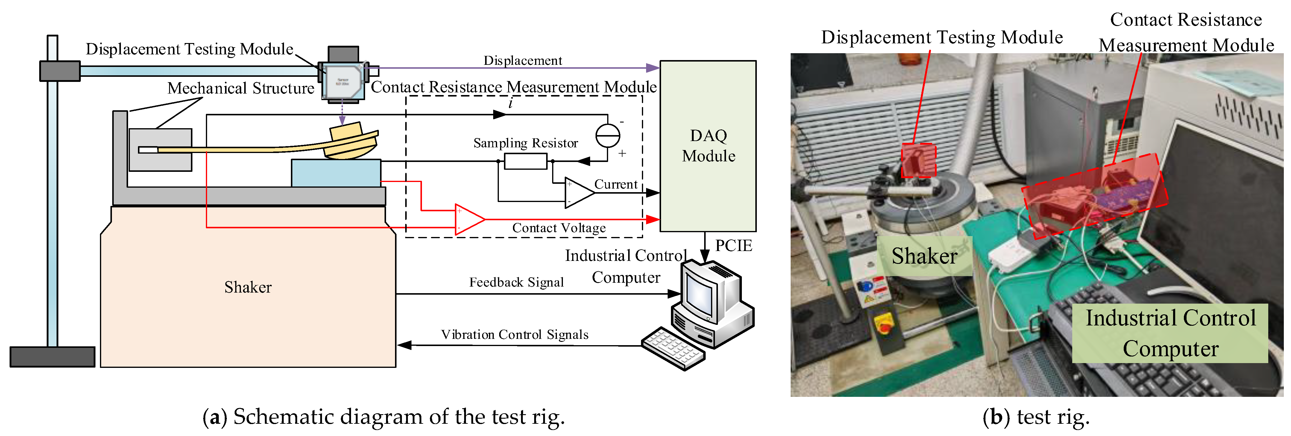
A laser confocal microscope (OLS3000, Olympus, Tokyo, Japan) is employed to scan and analyze the surface of the contact, and the acquisition of the surface height contour map is illustrated in Figure 10. The average roughness height is 12.84 μm, while the average slope is calculated as 0.5342. Moreover, the Brinell hardness of the contact material is measured to be 0.785 GPa by a microhardness tester.

Another commercial finite element software, COMSOL Multiphysics 5.6, was employed to simulate contact resistance. The material properties are determined based on the physical parameters, such as roughness and hardness, which have been tested previously. Subsequently, a sequence of contact force results is acquired through the adjustment of the overtravel. Coupled with the electrical module, the results of the contact resistance are obtained, as illustrated in Figure 11.

According to Holm’s theory [23], the contact resistance can be approximated by:

$$R_j=[H]F^{-n}$$

(28)

where [H] is dependent on the resistivity and hardness of the contact material and n is associated with the deformation of the contact surface, typically ranging from 0.5 to 1.

The simulation results are fitted to the fundamental form of Equation (28), which establishes the relationship between contact force and contact resistance specially used for AgSnO₂ cambered rivet and copper plane support, as follows:

$$R_j=7.4118F_n^{-0.9515}$$

(29)

in which the unit of contact resistance R_j is milliohms (mΩ) and the unit of contact force F_n is newtons (N).

As evident from the Equation (29), the contact resistance diminishes exponentially with a negative power as the contact force rises, and the magnitude of the exponent converges to 1.

4. Experiments

4.1. Experimental Details

Figure 12 shows the experiment system used for verifying the calculated vibration characteristics of the flexible beam structure. The whole test rig includes the shaker, the mechanical structure, the displacement testing module, the contact resistance measurement module, the DAQ module, the industrial control computer, and control software.

The spring structure specimen is illustrated in Figure 13. The straight spring material is beryllium bronze. A contact with cambered surface is riveted at the end of spring. A copper support block is used as the static contact. A laser displacement sensor (ILD2220-2, Micro-Epsilon, Ortenburg, Germany) is employed to measure the contact displacement during vibration, providing the measurement range of 0–2 mm with a resolution of 0.03 μm. The data is collected at a fixed frequency of 20 kHz.

The experimental conditions for vibration are listed in

Table 5. Experimental conditions.

Parameter	Value
Overtravel	0.2 mm
Testing voltage/current	6 V/100 mA
Sampling frequency	15.625 KS/s
Temperature	25 °C
Humidity	55% ± 5% RH

. A sequence of fixed-frequency vibration experiments is conducted, with the vibration acceleration amplitude of 98 m/s² and vibration frequencies of 500 Hz, 1000 Hz, 1500 Hz, and 2000 Hz.

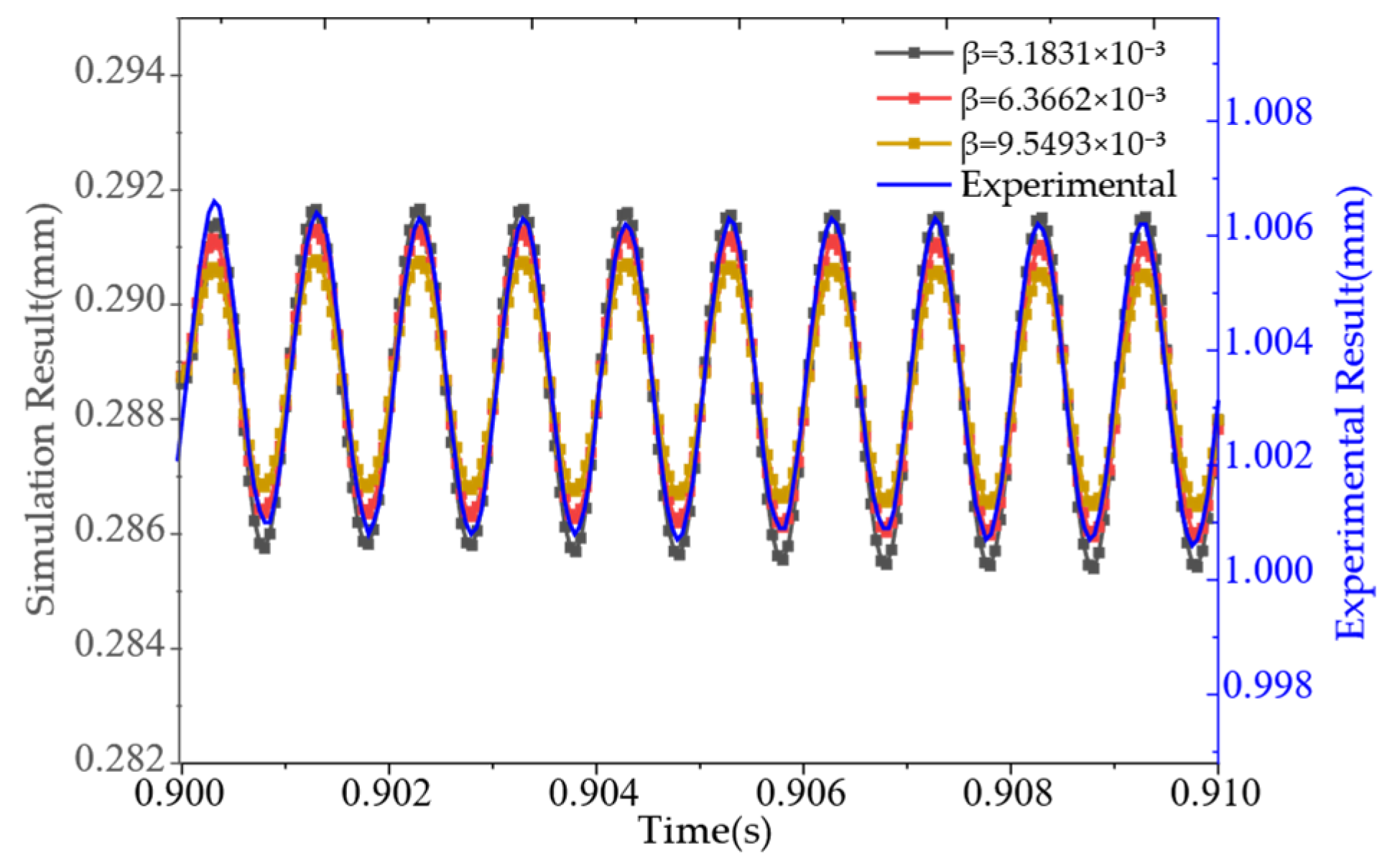
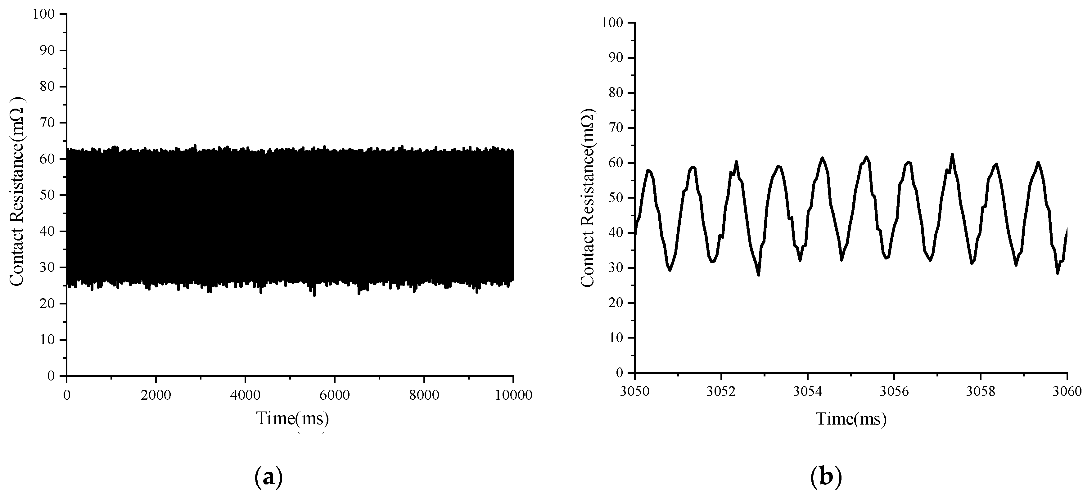
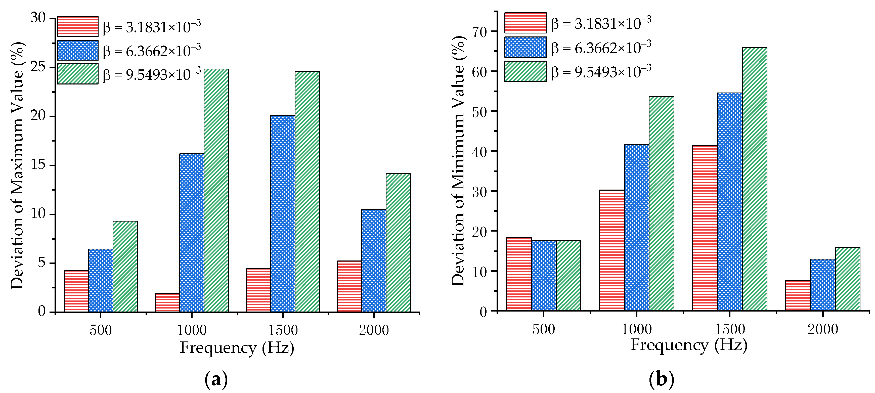
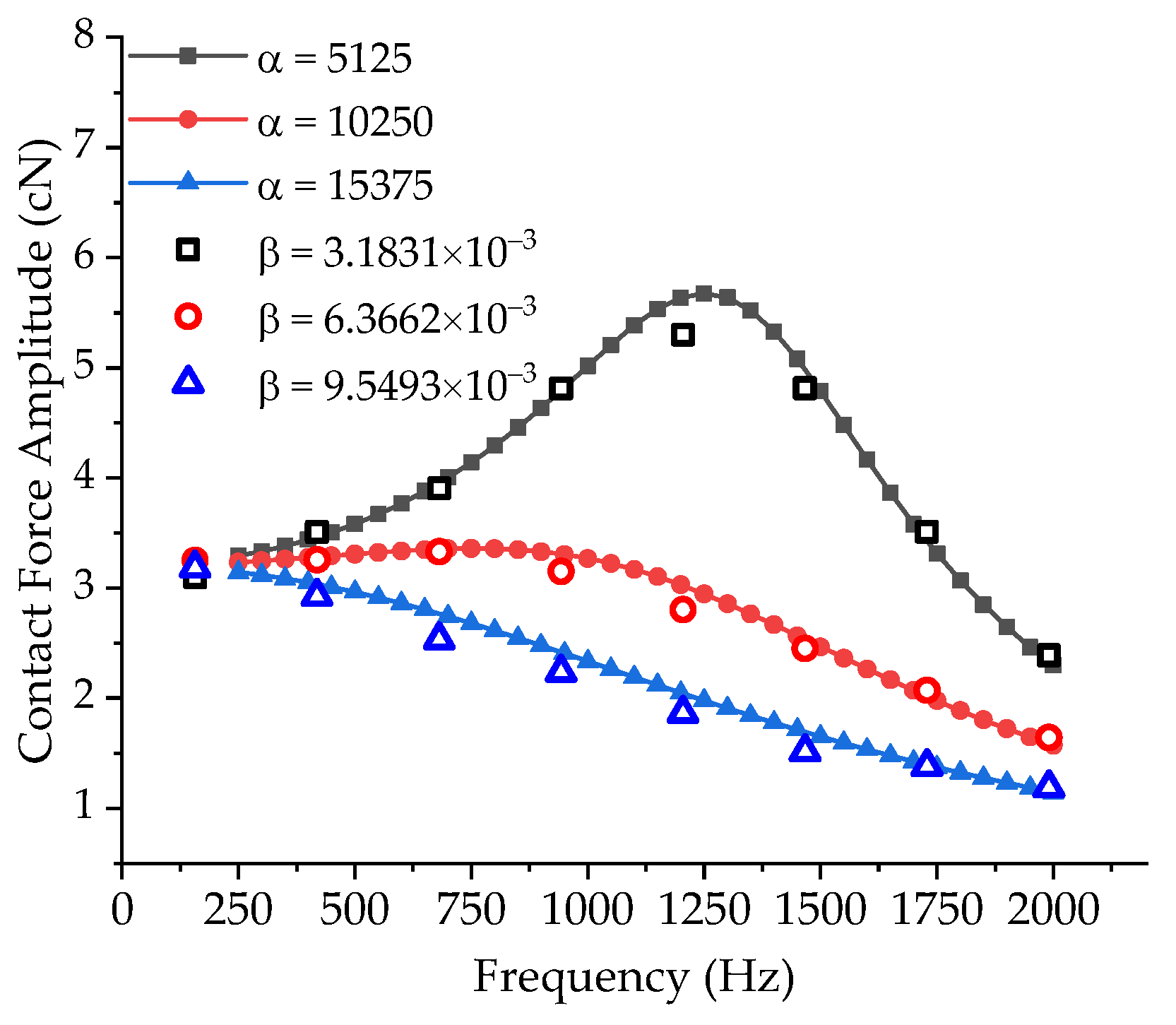
4.2. Results and Discussion

Figure 14 illustrates the results of the displacement tests for harmonic vibration contact, with a frequency of 1000 Hz. The experimental results indicate that the displacement response of the contact vibration exhibits a sinusoidal periodic vibration, with an amplitude of 0.0029 mm.

The displacement amplitudes acquired by the time domain simulation under damping conditions ranging from small to large are 0.003115 mm, 0.002632 mm, and 0.002524 mm, respectively. The deviations from the experimental values are 7.41%, 9.24%, and 12.97%. It is observed that the displacement results obtained from the simulation with a stiffness coefficient β of 3.1831 × 10⁻³ show the closest correlation to the experimental results.

The deviation between the experimental results and the time domain simulation results of the displacement response, with frequencies of 500 Hz, 1500 Hz, and 2000 Hz, is shown in Figure 15. When the stiffness coefficient β is set as 3.1831 × 10⁻³, the deviation between simulation results and experimental results is within 10%. The maximum deviation is 16.54% with β = 9.5493 × 10⁻³.

Figure 16 shows the results of the contact resistance measurement with a frequency of 1000 Hz. The fluctuation of the contact resistance ranges from 25 mΩ to 63 mΩ. Upon analyzing the waveform within the 10 ms range, it was observed that the contact resistance waveform exhibits periodic behavior with a period of approximately 1 ms. During the vibration process, the contact force undergoes sinusoidal changes over time, and the frequency of the fluctuation aligns with the external excitation frequency. Consequently, the contact resistance also exhibits periodic fluctuations with the same frequency.

The simulation results for contact resistance are derived by substituting the time domain contact force simulation outcomes into Equation (29) for computation. The deviations between these simulation results and the experimental results, as calculated using Equation (30), are presented in

Table 6. Deviation in contact resistance results.

Stiffness Coefficient β	Deviation of Minimum Contact Resistance Value (%)	Deviation of Maximum Contact Resistance Value (%)
3.1831 × 10−3	30.23	1.89
6.3662 × 10−3	41.63	16.18
9.5493 × 10−3	53.69	24.85

.

$$Dev={\displaystyle \frac{\left|R_s-R_e\right|}{R_e}}\times 100\%$$

(30)

where the Dev denotes the deviation between simulation result and experimental result, and R_s and R_e represent the simulation result and the experimental result, respectively.

As indicated in Table 5, the time domain simulation outcomes achieved using a stiffness damping coefficient of 3.1831 × 10⁻³ exhibit the closest resemblance to the experimental findings. The disparity between the time domain simulation results and the experimental results is illustrated in Figure 17. It is evident that the deviation of contact resistance maximum is less than 8%, and the deviation of contact resistance minimum is less than 40%, with a stiffness coefficient of 3.1831 × 10⁻³. The possible reason for the deviation of contact resistance between simulation and experiment is the neglection of film resistance in the simulation. Finally, the contact spring system investigated in this paper indicates that the time domain simulation method with the stiffness coefficient of 3.1831 × 10⁻³ provides a more precise estimation of the maximum contact resistance, which also indicates that this approach offers an acceptable level of reliability.

Similarly, the contact force results derived from the frequency domain simulation are utilized in Equation (29) to compute the contact resistance, which is compared with the experimental values. The resulting deviations are presented in Figure 18. As illustrated in the figure, when α = 5000, the simulation results in the frequency domain exhibit the least deviation from the experimental data, with a minimum deviation of 2.23% observed at 1500 Hz.

Furthermore, multiple sets of mass coefficients are utilized, with a value of approximately 5000 for the frequency domain simulation. It was determined that the maximum contact resistance value obtained through simulation exhibited the least deviation from the experimental maximum value when the mass coefficient was set at 5125. The deviations at frequencies of 500 Hz, 1000 Hz, 1500 Hz, and 2000 Hz are found to be 5.25%, 1.21%, 3.14%, and 7.13%, respectively.

A comparison of the simulation results with the experimental outcomes indicates that the deviation is minimized when the stiffness coefficient is set to 3.1831 × 10⁻³ and the mass coefficient is established at 5125. According to the definition of Rayleigh damping, the correlation between damping and the mass coefficient or stiffness coefficient in cases of utilizing mass damping or stiffness damping exclusively can be expressed as:

$$\left\{\begin{array}{l}{c}_t=\beta {\omega }_i^2(\alpha =0)\\ c_p=\alpha (\beta =0)\end{array}\right.$$

(31)

If we assume that the damping value in the time domain equals the damping value in the frequency domain, the corresponding relationship equation is:

$$\alpha =\beta {\omega }_i^2$$

(32)

Consequently, by establishing the mass coefficients at 10,250 and 15,375 for the frequency domain simulation, the resulting contact force amplitudes are compared with the previously obtained results from the time domain, as illustrated in Figure 19. The deviation between the results obtained from the two aforementioned methods is within 8%, suggesting a significant correlation between the two methods.

There is a direct correlation between the stiffness coefficient utilized in the time domain and the mass coefficient employed in the frequency domain within the model.

$$\alpha =1610065\beta$$

(33)

This approach facilitates the establishment of a connection between frequency do-main simulation and time domain simulation. Should the model’s size parameters undergo modifications, an initial small-scale time domain simulation, accompanied by a fixed frequency vibration test, can be conducted. The damping parameters for the time domain simulation can then be ascertained through a comparative analysis of the results. According to Equation (33), a linear relationship exists between the damping parameters in the frequency domain and those in the time domain. By comparing the outcomes of both frequency domain and time domain simulations, the damping parameters for the frequency domain simulation can be determined. Subsequently, frequency domain methods can be employed to efficiently and accurately resolve the harmonic vibration response of the model.

5. Conclusions

This paper presents a simulation analysis method to investigate the vibration characteristics of the flexible beam structure using a typical electromagnetic relay contact spring system as a case study. The effects of contact overtravel and free end length on fundamental frequency is investigated with the use of a prestressed modal simulation method. According to the principles of calculation in both the time domain and frequency domain, the stiffness damping coefficient is employed for time domain analyses, while the mass damping coefficient is utilized for frequency domain evaluations. Building upon this framework, the results pertaining to contact force amplitude and contact displacement amplitude at various frequencies are obtained. The variations in contact resistance of flexible beam structures under a mechanical vibration environment is measured and statistically analyzed. The experiment results demonstrate the feasibility of the proposed simulation method. There exists a linear correlation between the mass damping coefficient and the stiffness damping coefficient, as evidenced by a comparison of the results obtained from simulations and experimental studies.

References

1. Qiu, Z.-C.; Meng, F.-K.; Han, J.-D.; Liu, J.-G. Acceleration sensor-based first resonance vibration suppression of a double-clamped piezoelectric beam. Int. J. Acoust. Vib. 2016, 21, 11–23. [Google Scholar] [CrossRef]
2. Shi, H.; Fan, S.; Zhang, Y.; Sun, J. Design and optimization based on uncertainty analysis in electro-thermal excited MEMS resonant sensor. Microsyst. Technol. 2015, 21, 757–771. [Google Scholar] [CrossRef]
3. Gryzlov, A.A.; Grigor’ev, M.A. Improving the reliability of relay-protection and automatic systems of electric-power stations and substations. Russ. Electr. Eng. 2018, 89, 245–248. [Google Scholar] [CrossRef]
4. Liu, Y.Q. Research on the electromagnetic relay selection and reliability. In Proceedings of the 2015 International Power, Electronics and Materials Engineering Conference, Dalian, China, 16–17 May 2015. [Google Scholar]
5. Рoйзен. Miniature Sealed Electromagnetic Relay; Posts & Telecom Press: Beijing, China, 1979. [Google Scholar]
6. Chambega, D. A qualitative analysis on the effect of external vibrations on the performance of relays. In Proceedings of the IEEE. AFRICON’96, Western Cape, South Africa, 25–27 September 1996. [Google Scholar]
7. Ren, W.B.; Zhai, G.F.; Cui, L. Contact vibration characteristic of electromagnetic relay. IEICE Trans. Electron 2006, 89, 1177–1181. [Google Scholar] [CrossRef]
8. Nayak, P.R. Contact vibrations. J. Sound Vib. 1972, 22, 297–322. [Google Scholar] [CrossRef]
9. Szemplinska-Stupnicka, W. The Behavior of Nonlinear Vibrating Systems. Eng. Appl. Dyn. Chaos 1991, 1, 225–227. [Google Scholar]
10. Turner, J.A. Non-linear vibrations of a beam with cantilever-Hertzian contact boundary conditions. J. Sound Vib. 2004, 275, 177–191. [Google Scholar] [CrossRef]
11. Xie, F.; Flowers, G.T.; Chen, C.; Bozack, M.J.; Suhling, J.C.; Rickett, B.I.; Malucci, R.D.; Manlapaz, C. Analysis and prediction of vibration-induced fretting motion in a blade/receptacle connector pair. IEEE Trans. Compon. Packag. Technol. 2009, 32, 585–592. [Google Scholar] [CrossRef]
12. Rezaei, I.; Sadeghi, A. Vibrational behavior of atomic force microscope beam via different polymers and immersion environments. Eur. Phys. J. Plus 2021, 137, 72. [Google Scholar] [CrossRef]
13. Rezaei, I.; Sadeghi, A. Dynamic Behavior of Rectangular Atomic Force Microscope Cantilever by Supposing Diverse Polymeric Specimens and Immersion Media. J. Vib. Eng. Technol. 2022, 10, 2449–2479. [Google Scholar] [CrossRef]
14. Angadi, S.V.; Jackson, R.L.; Pujar, V.; Tushar, M.R. A comprehensive review of the finite element modeling of electrical connectors including their contacts. IEEE Trans. Compon. Packag. Technol. 2020, 10, 836–844. [Google Scholar] [CrossRef]
15. Echeverrigaray, F.G.; De Mello, S.R.S.; Leidens, L.M.; Boeira, C.D.; Michels, A.F.; Braceras, I.; Figueroa, C.A. Electrical contact resistance and tribological behaviors of self-lubricated dielectric coating under different conditions. Tribol. Int. 2020, 143, 106086. [Google Scholar] [CrossRef]
16. Almeida, A.; Donadon, M.; de Faria, A.; de Almeida, S. The effect of piezoelectrically induced stress stiffening on the aeroelastic stability of curved composite panels. Compos. Struct. 2012, 94, 3601–3611. [Google Scholar] [CrossRef]
17. Tchomeni, B.X.; Alugongo, A. Vibrations of misaligned rotor system with hysteretic friction arising from driveshaft–stator contact under dispersed viscous fluid influences. Appl. Sci. 2021, 11, 8089. [Google Scholar] [CrossRef]
18. Tomović, R. A simplified mathematical model for the analysis of varying compliance vibrations of a rolling bearing. Appl. Sci. 2020, 10, 670. [Google Scholar] [CrossRef]
19. Wnuk, M.; Iluk, A. Estimation of Resonance Frequency for Systems with Contact Using Linear Dynamics Methods. Appl. Sci. 2022, 12, 9344. [Google Scholar] [CrossRef]
20. Johnson, K.L. Contact Mechanics; Cambridge University Press: Cambridge, UK, 1987. [Google Scholar]
21. Ansys Inc. Ansys Help, Release 2021 R1; Ansys Inc.: Canonsburg, PA, USA, 2021; Available online: https://www.ansyshelp.ansys.com (accessed on 23 November 2024).
22. MIL-STD-202-204; Test Method Standard for Electronic and Electrical Component Parts. U.S. Department of Defense: Washington, DC, USA, 1980.
23. Holm, R. Electric Contacts: Theory and Application; Springer Science & Business Media: Berlin, Germany, 2013. [Google Scholar]
Figure 1. Normally closed contact pairs within the typical electromechanical relay.
Machines 13 00052 g001
Figure 2. Schematic of the flexible beam structure within the electromechanical relay. The set vertical offset causes a static beam deflection, y(x). The dynamic displacement, y(x,t), is defined relative to y(x). The contact between the two electrodes is assumed to be Hertzian contact.
Machines 13 00052 g002
Figure 3. Flexible beam structure model.
Machines 13 00052 g003
Figure 4. Modal shape of a beam with cantilever-Hertzian contact boundary conditions (f = 1354.5 Hz).
Machines 13 00052 g004
Figure 5. Modal frequencies under combination conditions of different free end length and overtravel.
Machines 13 00052 g005
Figure 6. Simulation results obtained by time domain analysis method (f = 1000 Hz, β = 3.1831 × 10⁻³).
Machines 13 00052 g006
Figure 7. Variations in contact force amplitude as a function of excited frequency by using the time domain method.
Machines 13 00052 g007
Figure 8. Deviation of the displacement amplitude obtained by the time domain method.
Machines 13 00052 g008
Figure 9. Variations in contact force amplitude as a function of exciting vibration frequency by using the frequency domain simulation method.
Machines 13 00052 g009
Figure 10. Contour map of contact surface measured by a laser confocal microscope.
Machines 13 00052 g010
Figure 11. The relationship between contact resistance and contact force.
Machines 13 00052 g011
Figure 12. Experiment system.
Machines 13 00052 g012
Figure 13. Contact spring specimen.
Machines 13 00052 g013
Figure 14. Displacement results (f = 1000 Hz). (Note: the distance between the displacement testing model and the measurement sample is 1.003 mm).
Machines 13 00052 g014
Figure 15. Deviation of displacement amplitude.
Machines 13 00052 g015
Figure 16. Experimental test contact resistance results (f = 1000 Hz). (a) 10 s contact resistance waveform. (b) Local contact resistance waveform within 10 ms.
Machines 13 00052 g016
Figure 17. Deviation between time domain simulation results and experimental results. (a) Deviation of maximum value. (b) Deviation of minimum value.
Machines 13 00052 g017
Figure 18. Deviation of maximum value between frequency domain simulation results and experimental results.
Machines 13 00052 g018
Figure 19. The amplitude results of contact force obtained by time domain analysis method and frequency domain analysis method.
Machines 13 00052 g019