Article

Prior-Guided Residual Reinforcement Learning for Active Suspension Control

1
CATARC (Tianjin) Automotive Engineering Research Institute Co., Ltd., Tianjin 300300, China
2
Technical Development Center, Shanghai Automotive Industry Corporation-General Motors-Wuling Automobile Co., Ltd., Liuzhou 545007, China
3
State Key Laboratory of Advanced Rail Autonomous Operation, Beijing Jiaotong University, Beijing 100044, China
4
The Department of Aeronautical and Aviation Engineering, The Hong Kong Polytechnic University, Hong Kong
*
Authors to whom correspondence should be addressed.
Machines 2025, 13(11), 983; https://doi.org/10.3390/machines13110983 (registering DOI)
Submission received: 16 September 2025 / Revised: 15 October 2025 / Accepted: 22 October 2025 / Published: 24 October 2025

Abstract

Active suspension systems have gained significant attention for their capability to improve vehicle dynamics and energy efficiency. However, achieving consistent control performance under diverse and uncertain road conditions remains challenging. This paper proposes a prior-guided residual reinforcement learning framework for active suspension control. The approach integrates a Linear Quadratic Regulator (LQR) as a prior controller to ensure baseline stability, while an enhanced Twin Delayed Deep Deterministic Policy Gradient (TD3) algorithm learns the residual control policy to improve adaptability and robustness. Moreover, residual connections and Long Short-Term Memory (LSTM) layers are incorporated into the TD3 structure to enhance dynamic modeling and training stability. The simulation results demonstrate that the proposed method achieves better control performance than passive suspension, a standalone LQR, and conventional TD3 algorithms.

1. Introduction

The suspension system plays a critical role in ensuring vehicle ride comfort, handling stability, and overall safety by isolating the vehicle body from road irregularities and maintaining consistent tire contact with the road surface [1,2,3]. Traditional passive suspensions, with fixed parameters, cannot alter the system dynamics, which limits their potential for performance improvement. In contrast, active suspensions can overcome these shortcomings by actively generating additional control forces to dynamically adjust the suspension performance. They have been widely applied in various vehicles to enhance ride comfort and driving stability [4,5,6].
Research on controlled suspension primarily centers on developing advanced control strategies and algorithms to maximize the performance potential of active suspension systems. Empirical control methods, such as Proportional–Integral–Derivative (PID) [7] and fuzzy PID [8], offer the advantages of simple structure, stable performance, and ease of engineering implementation, but they mainly rely on engineers’ experience and trial-and-error. In contrast, optimization-based suspension control methods, represented by Model Predictive Control (MPC) [9,10] and fractional-order SH-GH control strategy [11], achieve effective optimization of suspension system performance by constructing a dynamic model of the system and combining future state prediction with optimization algorithms, while satisfying various constraints. However, MPC requires full-state information obtained from additional sensors, which are costly in practice. When sensor measurements are limited, an advanced Kalman filter can be used to reconstruct the full states [12,13]. Furthermore, Linear Quadratic Regulator (LQR) control [14,15] has been introduced as an optimal control method that minimizes the quadratic cost function of state and control input, offering a trade-off between ride comfort and road holding. LQR control provides improved performance compared to PID, particularly under well-modeled linear system dynamics. In addition, considering model parameter uncertainties, some studies performed suspension control while simultaneously estimating the model parameters with typical estimation methods such as Kalman filtering [16,17].
The rapid advancement in artificial intelligence technologies, including reinforcement learning [18] and large language models [19], has brought data-driven learning approaches that provide engineers with new strategies and tools for tackling complex, knowledge-intensive tasks. The deep deterministic policy gradient DDPG algorithm has been applied to control strategies for full-vehicle active suspension configurations [20,21,22]. In addition, the soft actor-critic (SAC) [23] model has also been used to develop control strategies for complete-vehicle semi-active suspension systems. Experimental results show that this approach outperforms traditional algorithms in terms of performance. Furthermore, an increasing number of researchers are attempting to apply data-driven methods to the field of suspension control, for example, the Trust Region Policy Optimization (TRPO) [3], Proximal Policy Optimization (PPO) [24], and the TwinDelayed Deep Deterministic policy (TD3) [25]. In addition, although numerous studies have shown that data-driven deep reinforcement learning (DRL) holds great application potential, a major challenge lies in the interpretability of these methods. Some research has attempted to consider suspension safety under DRL control [26,27] to enhance reliability. However, in the field of automotive engineering, which requires rigorous verification and supervision, these techniques have yet to meet the necessary standards.
Based on the above analysis, traditional model-based suspension controllers offer strong interpretability but struggle with adaptability, while pure reinforcement learning methods, despite their high flexibility, suffer from low sample efficiency, slow convergence, limited stability guarantees in safety-critical scenarios, and poor interpretability. To address these issues, we propose a hybrid active suspension control approach that integrates LQR with policy learning. The main contributions are as follows:
(1)
A residual reinforcement learning (RRL) control method based on policy learning is proposed to enhance the control performance of the suspension system. This method combines a LQR controller to provide the baseline actuator force and incorporates reinforcement learning to generate a corrective control input, thereby improving the system’s adaptability and disturbance-rejection capability.
(2)
An improved TD3 model integrating residual connections and LSTM layers is proposed to enhance training stability and better capture the dynamic and inertial characteristics of the suspension system.
The rest of this paper is organized as follows. Section 2 presents the suspension model and the road model. Section 3 describes the proposed control framework. Section 4 shows the test results and discussion. Finally, Section 5 summarizes the work.

2. Active Suspension Model and Road Roughness Model

The vehicle can be simplified as a single-wheel, two-degrees-of-freedom vibration system, where the sprung mass (vehicle body) and the unsprung mass (wheel assembly) are connected via the suspension system. The suspension plays a critical role in ensuring both ride comfort and handling stability by maintaining adequate tire–road contact and attenuating road-induced vibrations. Although the quarter-car model is relatively simple, it effectively captures key dynamic characteristics such as tire dynamic load and suspension travel. Therefore, it is widely used to study the impact of active or active suspension control strategies on vehicle performance. The corresponding nonlinear model is illustrated in Figure 1.
The dynamic equations for vehicle suspension are
M X ¨ 2 + C ( X ˙ 2 X ˙ 1 ) + K ( X 2 X 1 ) = F
m X ¨ 1 C ( X ˙ 2 X ˙ 1 ) K ( X 2 X 1 ) + K t ( X 1 q ) + F = 0
where M represents the unsprung mass; m denotes the sprung mass; X ¨ 2 and X ¨ 1 are the corresponding accelerations which can be directly measured by sensors; K signifies the spring stiffness; K t symbolizes the tire stiffness q represents the ground excitation; C stands for the damping coefficient of the damper; the actuator’s force is F .
Rewriting Equations (1) and (2) into state-space form allows for the design of a LQR controller and a residual reinforcement learning controller. q is the interference term, and F L Q R is the output of the LQR.
x ˙ = A x + B u L Q R + H w y = C x + D u L Q R
x = [ X 2 X 1 ,   X ˙ 2   ,   X 1 q ,   X ˙ 1 ] T   u L Q R = [ F L Q R ] T
w = [ q ] T   y = [ X 2 X 1 ,   X ¨ 2 ,   X 1 q ] T
A = 0 , 1 , 0 , -1 K M , C M , 0 , C M 0 0 , 0 , 1 K m , C m , K t m , C m   B = 0 1 M 0 1 m   H = 0 0 1 0
C = 1 , 0 0 , 0 K M , C M , 0 C M 0 , 0 , 1 , 0   D = 0 1 M 0
In the development of vehicle systems, road surface modeling plays a pivotal role, particularly in suspension system design. To achieve accurate dynamic simulation, obtaining high-quality road excitation signals is essential. The precision of road modeling directly affects the reliability of suspension performance evaluation and overall vehicle dynamic behavior analysis. Currently, the Power Spectral Density (PSD) method is widely used for modeling stationary road surface irregularities. When a vehicle travels at a constant speed, the road profile can be abstracted as a random process in the spatial domain, typically assumed to follow a Gaussian distribution. The PSD technique effectively characterizes the energy distribution in the spatial frequency domain, thus providing a solid theoretical basis for modeling road surface irregularities [28]. PSD of road disturbance input can be represented by
G l n = G l n 0 n n 0 w
where n is the spatial frequency in m 1 ; n 0 is the reference of spatial frequency in m 1 ; G l n 0 is the power spectral density of road roughness; w represents the frequency index, m is the pavement waviness indicator.
According to the ISO standard classification, road roughness can be divided into five levels. The specific values of G l n 0 are listed in Table 1, below, when n 0 = 0.1   m 1 .
Furthermore, the relationship between the road excitation q , G l n 0 , and w is established through Equation (20) to complete the modeling of the road excitation [29].
q ˙ t + 2 π n 0 v c q t = 2 π n 0 G l n 0 v c w
where v c is the vehicle velocity.
The equation represents a standard road excitation model defined by the ISO, which is widely used for generating realistic stochastic road inputs in vehicle dynamics simulations. This model captures the statistical properties of road roughness and allows for the consistent generation of road profiles across different roughness classes. It is particularly useful for testing and validating suspension control systems under repeatable conditions, making it a valuable tool in the development and evaluation of advanced suspension control strategies.

3. Methodology

As shown in Figure 2, a residual reinforcement learning (RRL) control strategy is proposed for the active suspension system to enhance its performance. This approach consists of a conventional Linear Quadratic Regulator (LQR) controller and an improved TD3 (Twin Delayed Deep Deterministic Policy Gradient) reinforcement learning network. The output of the LQR controller serves as the baseline control signal for the entire control scheme. The improved TD3 reinforcement learning component is then employed to address the performance degradation of the LQR controller caused by its fixed gain when facing random road excitations of varying severity. Furthermore, considering the presence of inertial elements in the suspension system, LSTM (Long Short-Term Memory) layers are integrated into both the Actor and Critic networks in the TD3 architecture to better capture the dynamic evolution of the suspension system. Compared with the general RRL framework, the proposed hybrid structure incorporates an improved TD3 algorithm to adaptively optimize the residual control signal and enhance robustness under complex road excitations. In addition, LSTM layers are embedded in both the Actor and Critic networks to capture the temporal dependencies of suspension dynamics, which is rarely considered in existing RRL frameworks. To the best of our knowledge, this hybrid algorithm has not yet been reported for active suspension control.

3.1. The Residual Policy Learning Control

While LQR provides optimal control performance under known linear system dynamics and predefined cost functions, its effectiveness significantly degrades when the system is subject to nonlinearities, time-varying parameters, or unmodeled disturbances, conditions that frequently arise in real-world road situations. In such cases, purely model-based control may lack the adaptability required for maintaining optimal ride comfort and road holding. Therefore, a policy learning control is adopted for the active suspension control, where the final control action is composed of an LQR output combined with a corrective residual term generated by an improved TD3. The improved TD3 incorporates memory-aware structures (e.g., LSTM layers) into the Actor–Critic networks, allowing the policy to capture temporal dependencies in the suspension dynamics and external disturbances. This residual learning scheme enables the controller to exploit the efficiency and stability of LQR while compensating for its limitations through data-driven adaptation. The final suspension control force F is calculated as follows:
F = u L Q R + Δ F = u L Q R + a t
where u L Q R is the output of LQR; Δ F is represents the actuator force correction term, which is generated by the improved TD3 algorithm; a t is the output of the improved TD3.

3.2. The LQR Controller

The LQR is a widely adopted optimal control strategy in suspension systems due to its ability to systematically minimize a quadratic cost function that balances ride comfort, road holding, and control effort. By utilizing a state-space model of the suspension dynamics, LQR computes an optimal feedback-gain matrix that ensures stable performance under known and stationary system conditions. In the context of active suspension control, LQR effectively attenuates body acceleration and suspension deflection in response to road disturbances, achieving a desirable trade-off between comfort and stability. Based on the suspension dynamics model, optimizing suspension performance involves three key indicators: acceleration of the unsprung mass, suspension deflection, and tire deflection. These indicators are negatively correlated with suspension effectiveness; lower values indicate better performance. To quantitatively evaluate their impact, mathematical formulations are introduced, as shown in Equation (7).
J = lim T 1 T 0 T σ 1 X 2 X 1 2 + σ 1 X ¨ 2 2 + σ 3 X 1 q 2 Γ u L Q R 2 d t
Equation (7) can be transformed into Equation (8).
J = lim T 1 T 0 T y T ρ y + u L Q R T Γ u L Q R d t = lim T 1 T 0 T C x + D u L Q R T ρ C x + D u L Q R + u L Q R T Γ u L Q R d t = lim T 1 T 0 T C x + D u L Q R T ρ C x + D u L Q R + u L Q R T Γ u L Q R d t = lim T 1 T 0 T x T C T ρ C x + 2 x T C T ρ D u L Q R + u L Q R T D T ρ Q D + Γ u L Q R d t
Let ρ = d i a g σ 1 , σ 2 , σ 3 , ρ ˜ = C T ρ C , N = C T ρ D and Γ ˜ = D T ρ D + Γ . Equation (8) can be rewritten as Equation (9).
J = lim T 1 T 0 T x T ρ ˜ x + 2 x T N u L Q R + u L Q R T Γ ˜ u L Q R d t
Once the weighting coefficients for the vehicle parameters and performance indices are specified, the optimal state feedback-gain matrix can be derived by solving the Riccati equation.
P A + A T P P B + N Γ ˜ P B + N T + ρ ˜ = 0
The optimal control feedback gain K ˜ is given by the following:
K ˜ = Γ ˜ 1 B T P + N T
The optimal control force F L Q R is as follows:
F L Q R = K ˜ x

3.3. The Improved TD3

An enhanced version of the TD3 algorithm was utilized to improve the control performance of the vehicle suspension system. In this framework, the suspension system is treated as an agent whose control policy is not predefined but instead learned through continuous interaction with a simulated environment. The learning process is framed as a Markov Decision Process (MDP), which is characterized by a set of states S , actions A , and rewards R . At each discrete time step t, the current state s t S is observed, and a corresponding action a t A is selected based on the learned policy. As a result of this action, the system transitions to a new state s t + 1 and a numerical reward r t R is issued by the environment, reflecting the quality of the action taken. The overarching objective is to discover a policy that maximizes the expected cumulative reward R t = i r t γ t i ,   γ 0 , 1 over time. Further methodological details are provided below.
Suspension control, ride comfort, and road handling are typically the primary performance criteria to consider. As a result, it is necessary to monitor the acceleration and displacement signals in real time. Accordingly, the state variables are defined as follows:
S t = [ X 2 ( t ) X 1 ( t ) ,   X ˙ 2 ( t )   ,   X 1 ( t ) q ( t ) ,   X ˙ 1 ( t ) ] T
For active suspension systems, the primary control input is the force applied by the actuator. Since a residual reinforcement learning framework is adopted, the action space of the TD3 controller corresponds to the residual force adjustment, which is applied on top of an LQR controller. Therefore, the action space is defined as the following:
A t = [ Δ F ] T
The reward function is a critical component of the reinforcement learning algorithm, as it guides the learning direction of the agent and influences the convergence speed of the algorithm. In this study, the primary objective is to enhance the suspension comfort while optimizing the control input energy. Accordingly, a continuous reward function is designed as follows:
r t = X ¨ 2 ( t ) 2 + 0.5 X 1 ( t ) q ( t ) 2 + 0.01 Δ F 2
denotes the normalization operation applied to each individual variable.
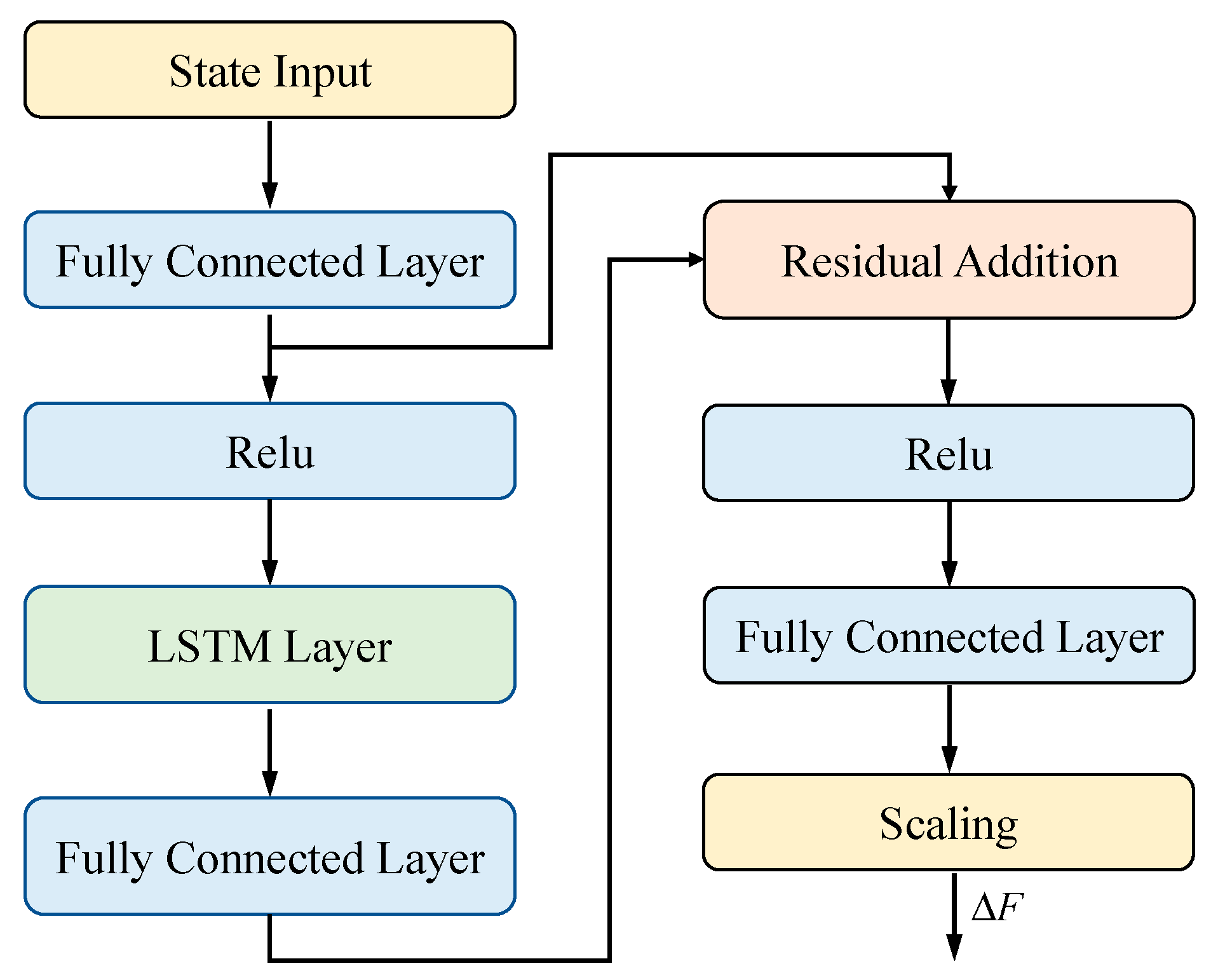
In active suspension control, incorporating residual connections into the Actor network of TD3 can improve the training stability and policy performance. This structure mitigates the vanishing gradient problem by adding shallow and deep features, enhancing the network’s ability to model nonlinear characteristics and adapt to dynamic changes under complex road conditions. Furthermore, introducing LSTM layers into the TD3 controller improves the system’s capacity to model temporal dependencies, system inertia, and environmental nonlinearity, making it particularly suitable for tasks like vehicle suspension control, which involve delays, partial observability, and dynamic variations. Figure 3 illustrates the detailed architecture of the Actor network, which is composed of fully connected layers, an LSTM layer, and residual addition connections. Specifically, the LSTM layer contains 64 hidden units, and the sequence length corresponds to the time window of the input data used during training. All LSTM weights and biases are initialized using the Glorot (Xavier) uniform initialization scheme, which helps maintain stable gradient propagation and ensures efficient network convergence.
Disturbances under complex road conditions—such as continuous undulations and potholes—often exhibit certain patterns. The LSTM is capable of recognizing these dynamic patterns, enabling the Critic to more accurately evaluate future returns and guide the Actor in learning more robust control policies. Additionally, real-world suspension systems are subject to significant sensor noise and structural inertia. By integrating long-term information, the LSTM can suppress the influence of transient anomalies on Q-value estimation within the Critic network. Figure 4 shows the architecture of the Critic network, which is composed of an LSTM, a concatenation layer, and multiple fully connected layers.
The TD3 algorithm is an improved version of the DDPG designed for continuous action spaces. It follows an actor-critic architecture, consisting of one actor network and two critic networks. The actor network maps states to actions and represents the policy, while the two critic networks estimate Q-values to evaluate the quality of actions. To reduce the overestimation bias common in Q-learning methods, TD3 uses the minimum value between the two critics during the target value calculation. Additionally, it employs target networks for both the Actor and Critics to improve training stability. TD3 also delays the actor’s update and adds noise to the target policy to prevent the exploitation of value function errors, enhancing robustness and performance. The actor network is denoted as μ s | ϑ μ with parameter ϑ μ ; the critic network Q s , a | ϑ Q with parameter ϑ Q . The corresponding target networks for the actor and critic networks are denoted as μ ˜ s | ϑ μ ˜ and Q ˜ s , a | ϑ Q ˜ , respectively. In the TD3 algorithm, let the two critic networks be denoted as Q 1 s , a | ϑ Q 1 and Q 2 s , a | ϑ Q 2 , and their corresponding target networks as Q ˜ 1 s , a | ϑ Q ˜ 1 and Q ˜ 2 s , a | ϑ Q ˜ 2 , respectively. The updates for the two different action-value estimates from critic networks are as follows:
Q ˜ 1 s t + 1 , a t + 1 | ϑ Q ˜ 1 = Q ˜ 1 s t + 1 , μ ˜ s t + 1 | ϑ μ ˜ | ϑ Q ˜ 1 Q ˜ 2 s t + 1 , a t + 1 | ϑ Q ˜ 2 = Q ˜ 2 s t + 1 , μ ˜ s t + 1 | ϑ μ ˜ | ϑ Q ˜ 2
To further compute the loss functions for the two critic networks in the TD3 algorithm, we proceed as follows:
χ t = r ( s t , a t ) + γ min i = 1 , 2 Q ˜ i s t + 1 , a t + 1 | ϑ Q ˜ i
L ϑ Q ˜ i = E χ t Q ˜ i s t , a t | ϑ Q ˜ i | a t = μ ˜ s t | ϑ μ ˜ 2
where r denotes the one-step reward; χ t is the target Q value at the specific state; L ϑ Q ˜ i is the loss function; E is the mathematical expectation; γ is the discounting factor.
The parameters of ϑ Q i are updated by minimizing the L ϑ Q ˜ i using gradient descent. This process can be expressed as
L ϑ Q ˜ i = E χ t Q ˜ i s t , a t | ϑ Q ˜ i Q ˜ i s t + 1 , a t + 1 | ϑ Q ˜ i | i = 1 , 2 ϑ Q ˜ i ϑ Q ˜ i α L ϑ Q ˜ i
where L ϑ Q ˜ i denotes the gradient of L ϑ Q ˜ i ; Q ˜ i s t + 1 , a t + 1 | ϑ Q ˜ i denotes the gradient of ϑ Q ˜ i ; α is the learning rate.
To further maximize the expected reward, the parameters of ϑ μ are updated using gradient ascent as follows:
J ϑ u = E Q 1 s t , a | ϑ Q 1 | a = μ s t | ϑ μ μ s t | ϑ μ J = E i = t T γ i t r s i , a i , ϑ u ϑ u + β J ϑ u
where J ϑ u denotes the gradient of J ϑ u ; Q 1 s t , a | ϑ Q 1 denotes the gradient of the Q value; μ s t | ϑ μ denotes the gradient of the policy μ ; β is the learning rate.
To smooth Q-value estimation, alleviate overfitting and overestimation, and thereby improve the stability and generalization of the policy, noise should be added to the target critic network, which is formalized as the following:
a t + 1 = μ ˜ s t + 1 | ϑ μ ˜ + ξ ,   ξ c l i p N 0 , σ , c , c
In the parameter update strategy of the TD3 algorithm, the update frequency of the actor and target networks is reduced, and their updates are performed only after the critic networks have been updated for a fixed number of steps. In this way, the update of the critic networks is stabilized, and the quality of the resulting policy is effectively improved.
ϑ Q ˜ i τ ϑ Q ˜ i + ( 1 τ ) ϑ Q ˜ i ϑ u ˜ τ ϑ u ˜ + ( 1 τ ) ϑ u ˜
where τ is the soft updating factor.
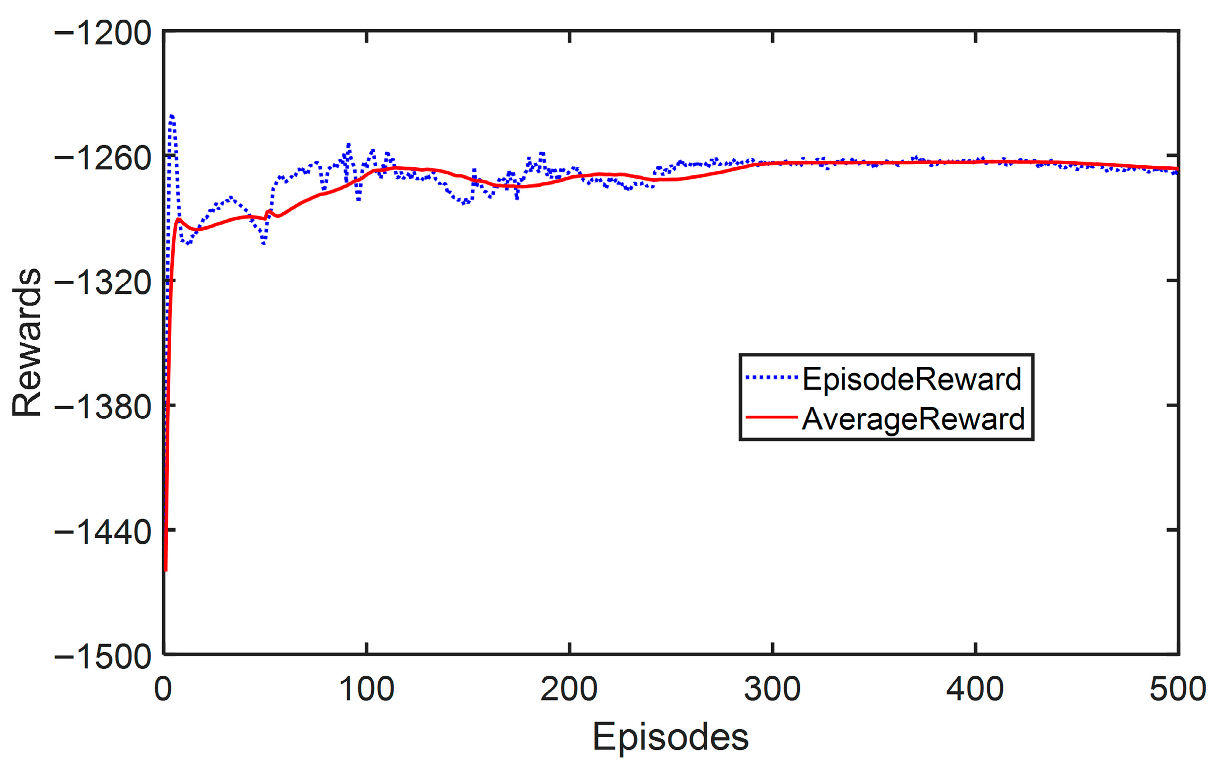
The parameters for the improved TD3 and LQR algorithms used to train the controller are presented in Table 2. Figure 5 shows the training process. “Episode reward” is the reward for each episode, and “Average reward” is the average reward of every 20 episodes.

4. Results and Discussion

An active suspension model was developed using a mainstream simulation platform. To evaluate the effectiveness of the proposed control method, three different control strategies are considered: passive suspension (with no control input), LQR control, TD3 control, and residual reinforcement learning control. The suspension performance under each control strategy is assessed using two different types of road excitation. The relevant suspension parameters are as follows in Table 3.

4.1. The Test on Class B Road

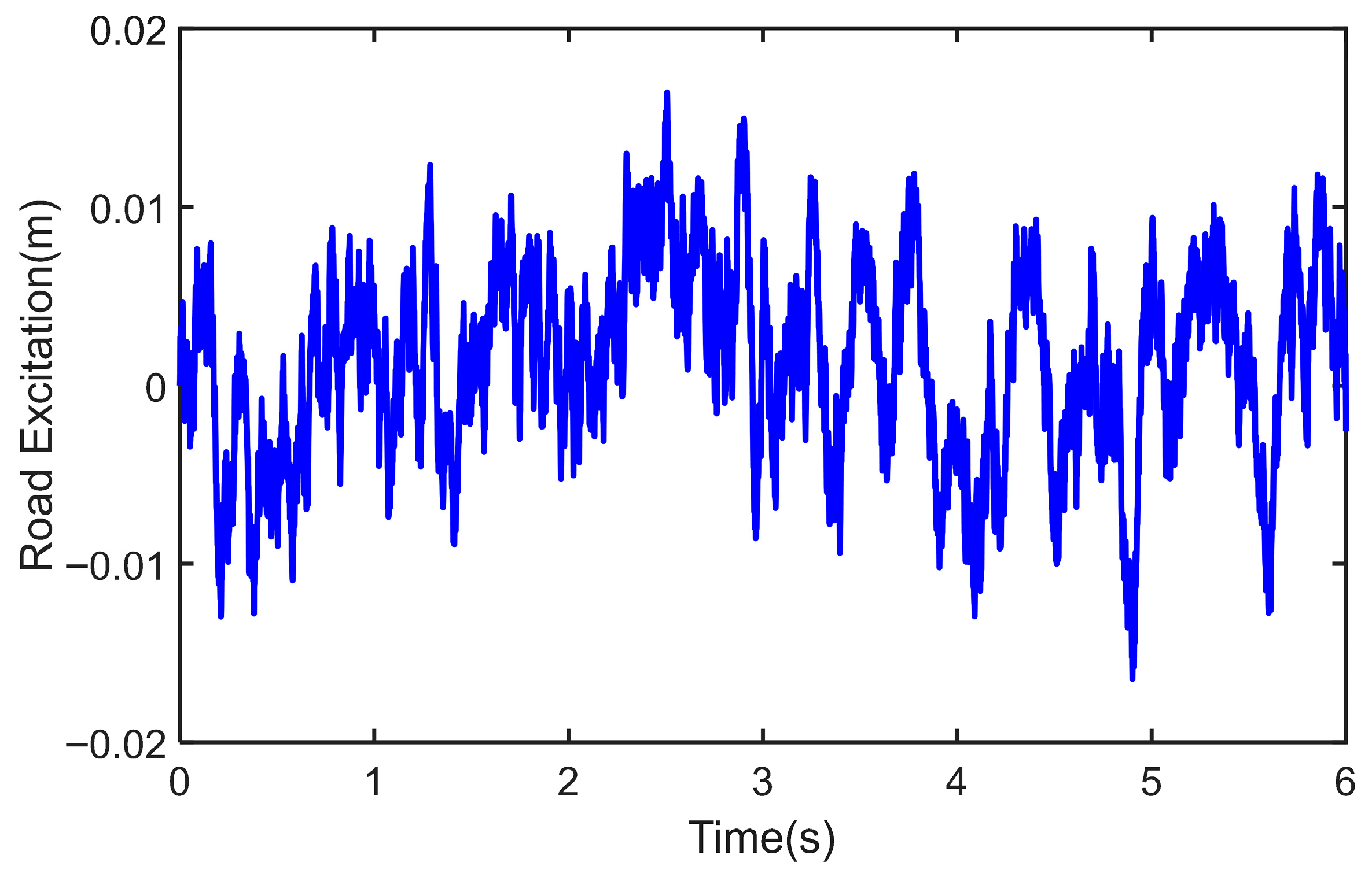
The vehicle speed is set to 80 km/h, and the road excitation is based on an ISO Class B road surface. Figure 6 shows the road excitation profile. As it is a randomly generated surface, the curve exhibits irregular variations. The range of excitation fluctuations lies between −0.02 and 0.02 m.
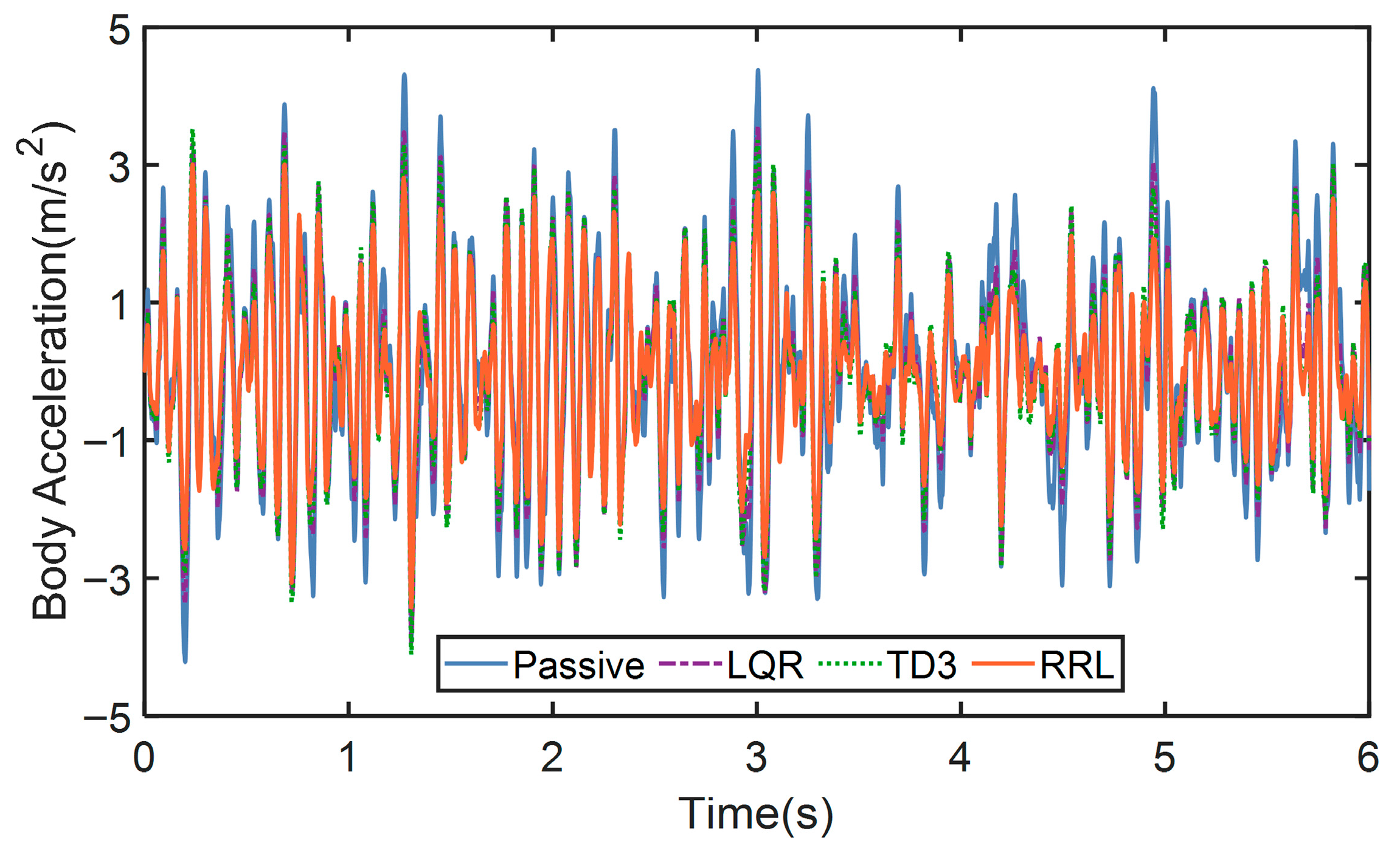
Figure 7 illustrates the variation in body acceleration under different suspension control algorithms. The light blue solid line represents the passive suspension case, where the suspension system applies no additional control and relies solely on the spring and damper to respond to road excitations. The purple dash-dot line shows the result of using the LQR control alone, the green dashed line corresponds to the result obtained using the TD3 algorithm independently, and the red solid line represents the performance of the proposed residual reinforcement learning (RRL) approach, which combines LQR with the improved TD3 algorithm. As shown in Figure 7, the acceleration amplitude under LQR control is lower than that of the passive suspension, and the TD3-based result is further reduced compared with the LQR method. Moreover, the proposed RRL algorithm achieves the lowest acceleration amplitude, indicating its superior control performance. This improvement can be attributed to the fact that the fixed gain of the LQR controller may lead to performance degradation under unknown disturbances, while the residual reinforcement learning component effectively compensates for such variations and enhances the overall control performance.
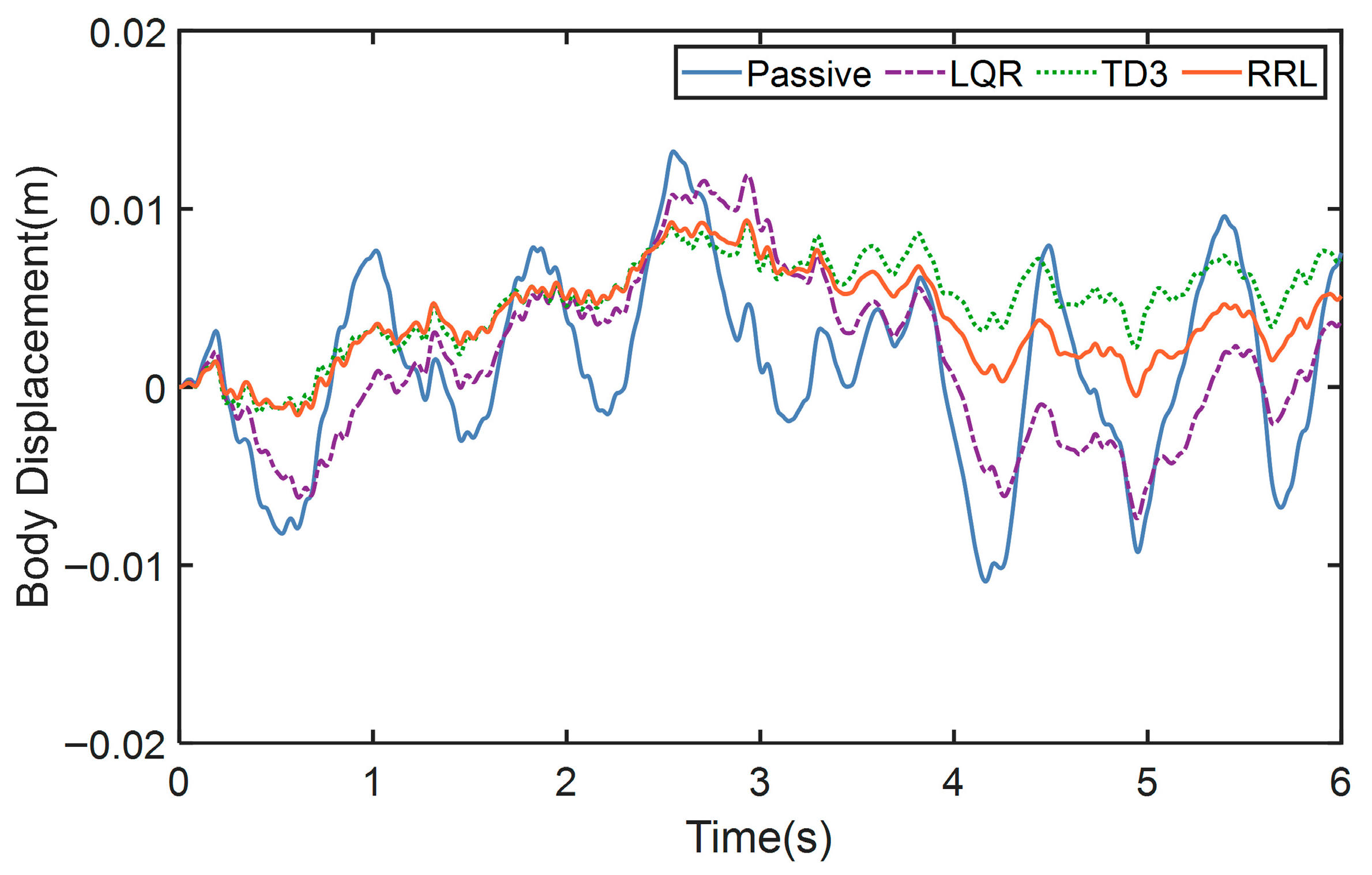
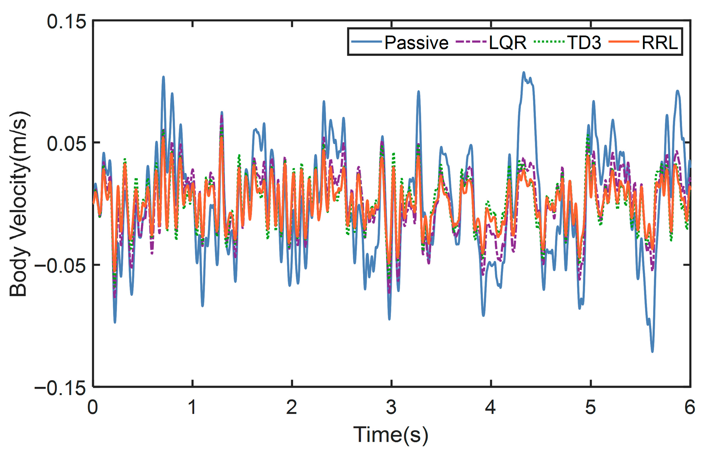
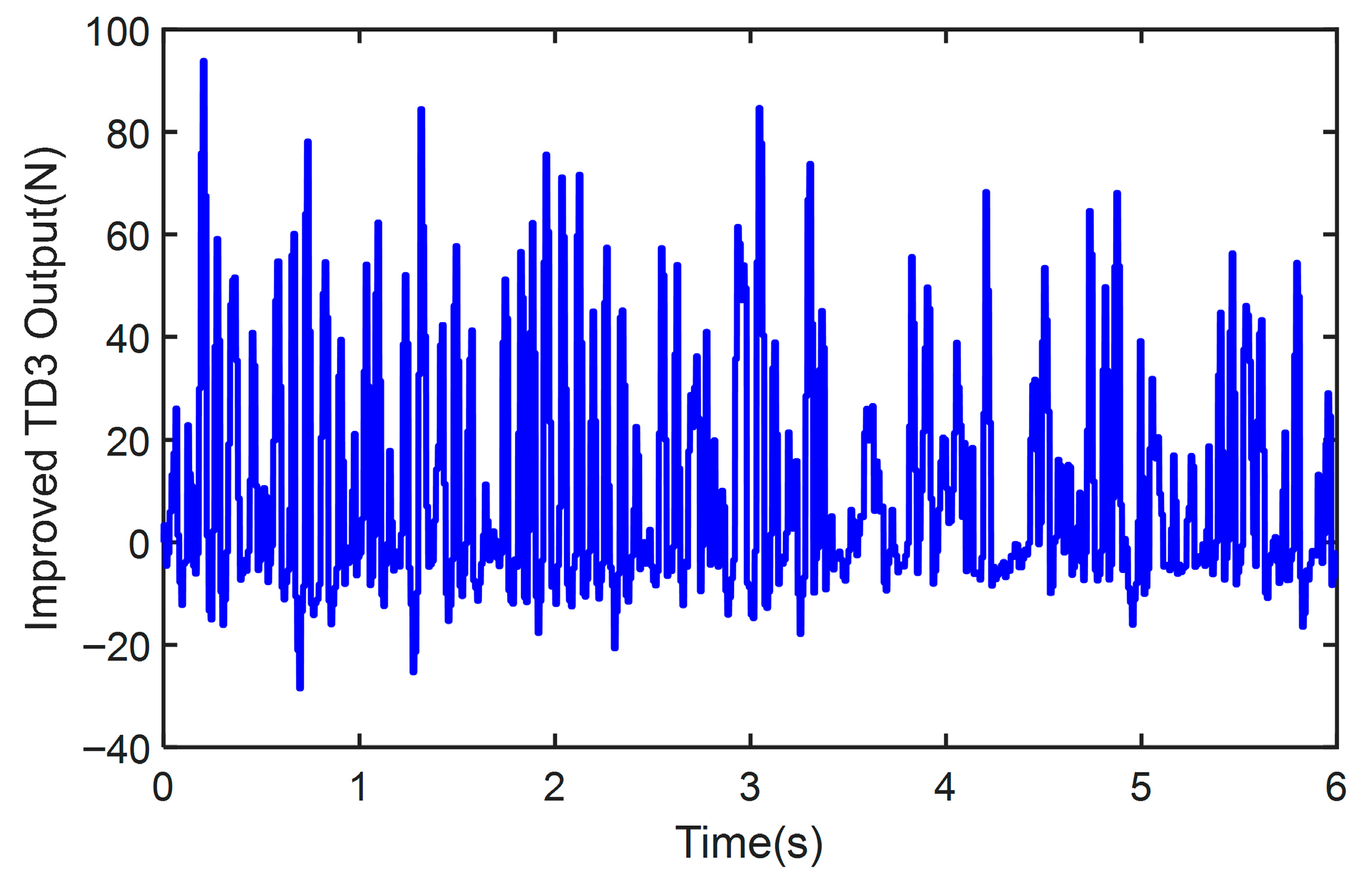
Figure 8 illustrates the variation in body displacement, with the curve definitions consistent with those in Figure 6. It can be observed that the displacement amplitude under RRL control is lower than that under TD3, LQR, and passive suspension, indicating that the RRL-based control achieves the best performance in minimizing body displacement. Figure 9 presents the body velocity responses under the three different control strategies, where the velocity curve corresponding to the RRL control exhibits the smallest amplitude. This demonstrates that RRL also achieves superior performance in reducing body velocity fluctuations. Figure 10 shows the real-time control force generated by the improved TD3 algorithm within the RRL control framework. This force, together with the LQR output, constitutes the total control input of the RRL controller. It can be seen that the improved TD3-generated control force continuously adapts to road excitations, ensuring that the RRL controller maintains optimal performance at all times.
To further quantify the performance of the control algorithms, the Root Mean Square (RMS) values are presented in Table 4.
As shown in Table 4, the use of RRL control can significantly reduce the RMS values of body acceleration, displacement, and velocity. The RMS values under the RRL algorithm are lower than those of TD3, LQR, and passive suspension. Compared with the passive suspension, RRL active control reduces the RMS of body acceleration, displacement, and velocity by 28.3286%,13.1371% and 60.4671%, respectively.

4.2. The Test on Class E Road

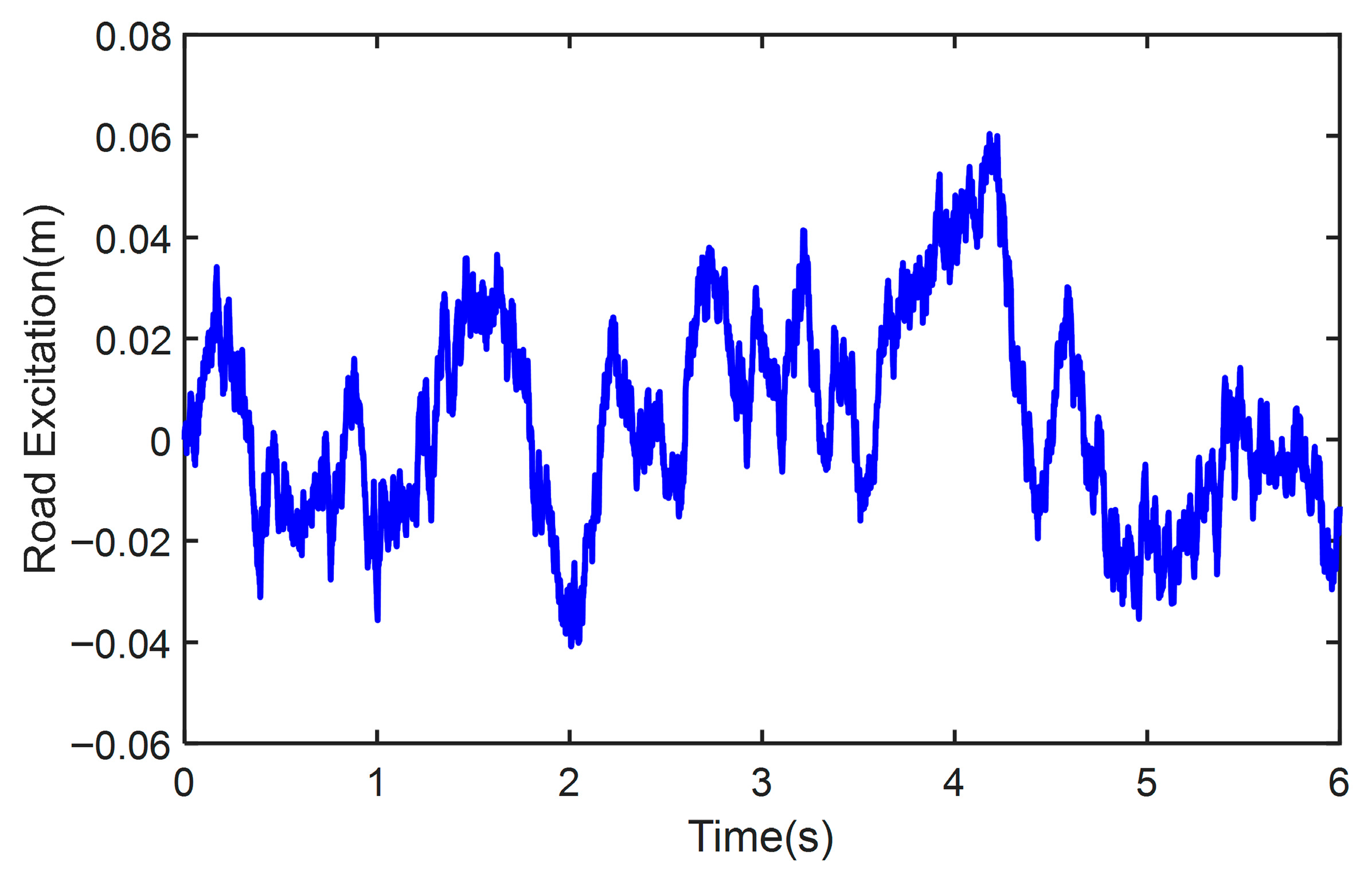
The vehicle operates at a speed of 15 km/h, with road excitation modeled using an ISO Class E road surface. As illustrated in Figure 11, the excitation profile displays irregular variations due to the stochastic nature of the surface generation. The amplitude of these fluctuations ranges from −0.05 to 0.08 m. It can be observed that the ISO Class E road surface induces larger excitation amplitudes, which place higher demands on the active suspension control system. By comparing different operating conditions, the applicability and robustness of the proposed control algorithm can be validated.
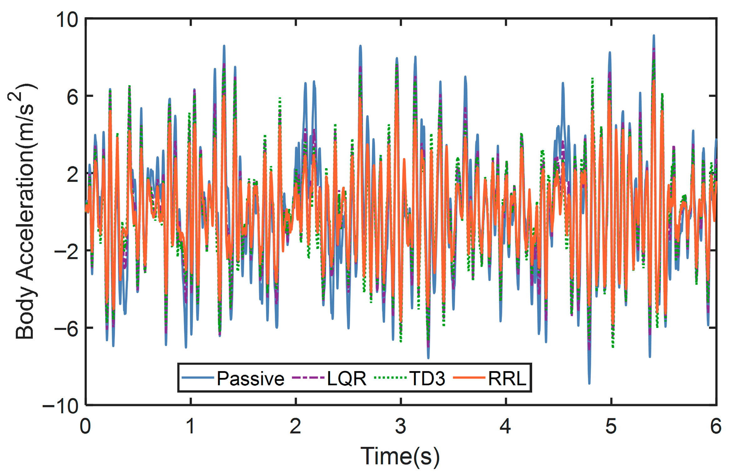
Figure 12 illustrates the vehicle body acceleration curves under four control strategies when subjected to Class E road excitation, with the curve definitions consistent with those in Section 4.1. As shown in the Figure, the passive suspension exhibits the largest acceleration fluctuations, which are significantly higher than those under Class B road excitation due to the stronger disturbances introduced by the Class E surface. In contrast, the LQR-controlled suspension effectively reduces body acceleration, while the TD3 control achieves better performance than LQR. Furthermore, the RRL control strategy demonstrates the best overall performance.
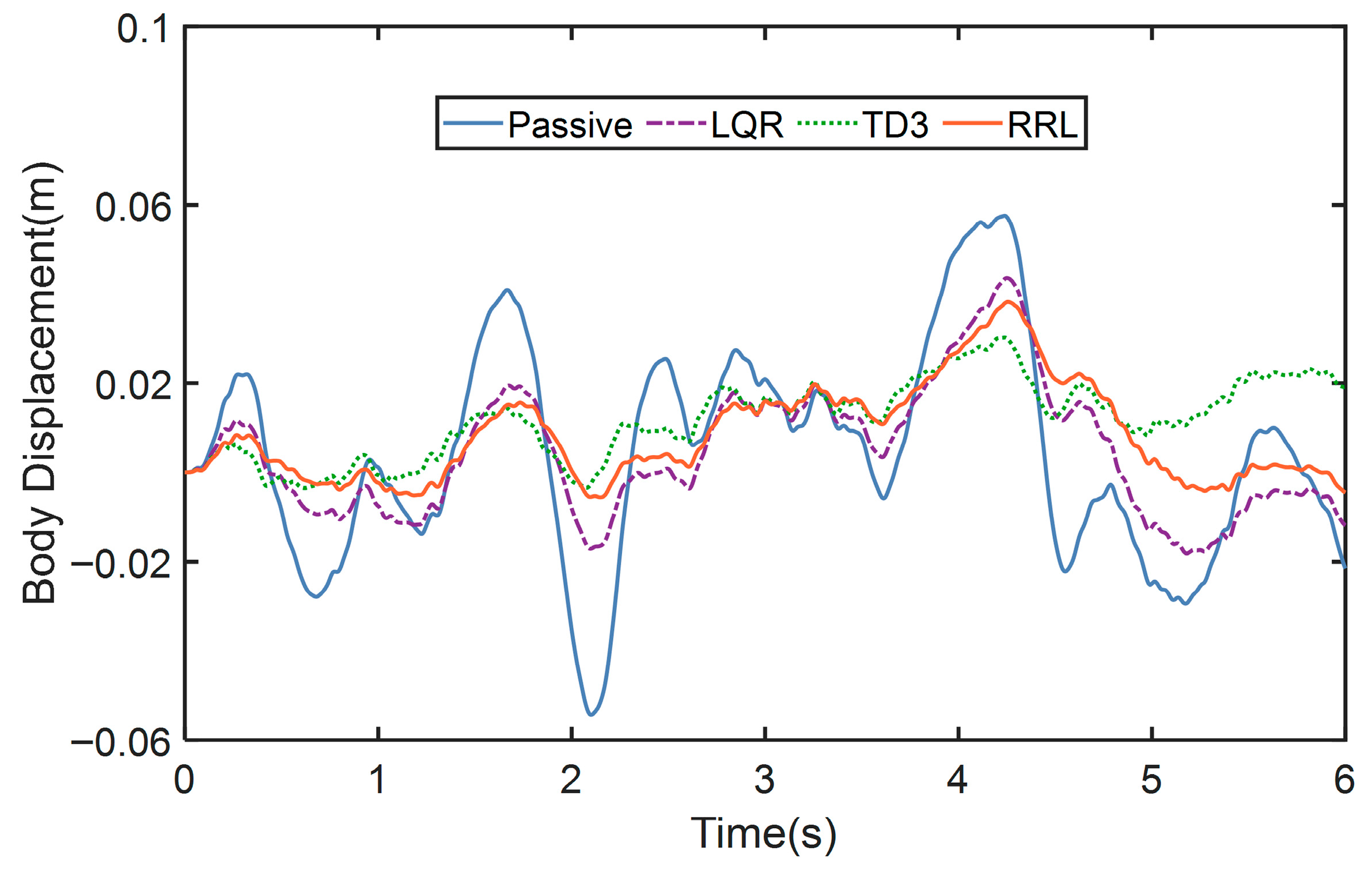
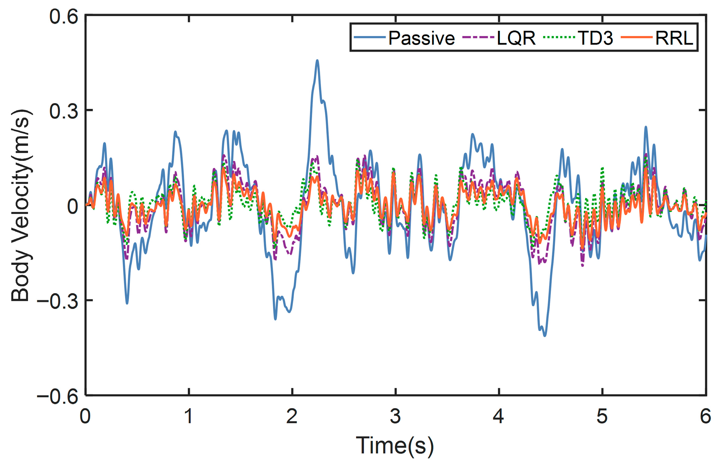
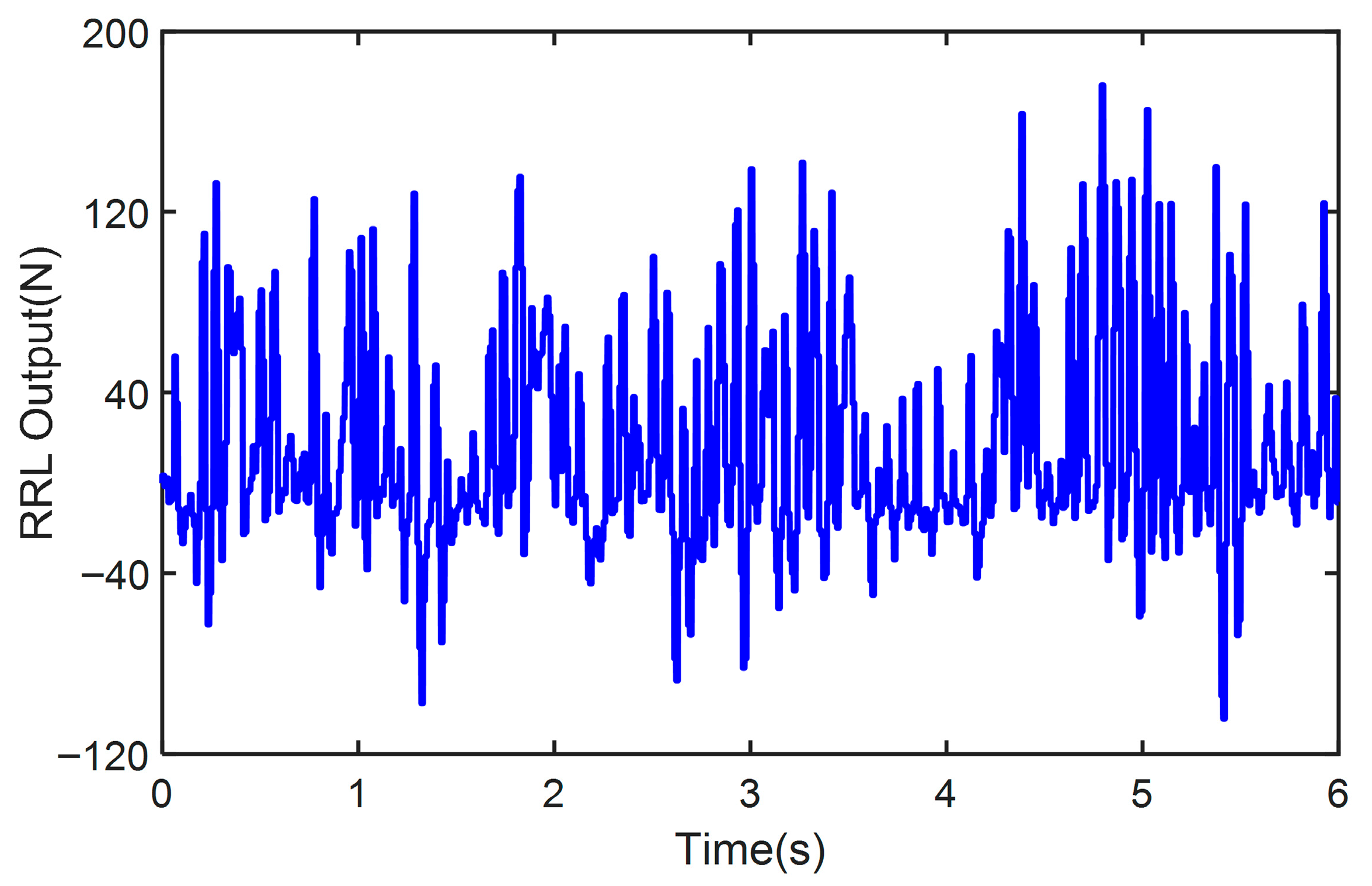
Figure 13 illustrates the vehicle body displacement responses under four different control strategies. As shown, the passive suspension exhibits the largest peak displacement, while the other three methods significantly reduce the peak value. Among them, the RRL control achieves better performance than both LQR and TD3, indicating that the RRL approach has a stronger capability to suppress external disturbances. Figure 14 presents the vehicle body velocity responses under the four control strategies. Similarly to the results of other variables, the RRL-based control demonstrates the best performance, showing the smallest velocity fluctuations and amplitudes, which further verifies the effectiveness of the RRL strategy. Figure 15 shows the real-time control outputs of the improved TD3 model. It can be observed that the outputs vary in real time according to changes in road excitation. Due to the larger fluctuations associated with the ISO Class E road surface, the corresponding control outputs exhibit greater amplitudes compared with those under Class B excitation. This demonstrates that the improved TD3 model can dynamically adapt to varying operating conditions. To further quantify the performance of the control algorithms, the RMS values are presented in Table 5.
As shown in Table 5, the use of RRL control can significantly reduce the RMS values of body acceleration, displacement, and velocity. The RMS values under the RRL algorithm are lower than those of TD3, LQR, and passive suspension. Compared with the passive suspension, RRL active control reduces the RMS of body acceleration, displacement, and velocity by 31.5988%, 43.2449%, and 68.1833%, respectively.
The results under both road excitation conditions demonstrate that the RRL-based control strategy consistently achieves superior performance compared to the other methods. This indicates that the proposed approach is not only adaptable to varying operating scenarios but also effective in attenuating the influence of unknown disturbances with different magnitudes. These findings underscore the enhanced robustness and generalization capability of the proposed algorithm across diverse road conditions.

5. Conclusions

In this article, a residual policy learning framework for active suspension systems is presented to overcome the limitations of traditional model-based and pure reinforcement learning methods. The effectiveness of the proposed method is validated through extensive simulations under various road conditions, where superior control performance and robustness are demonstrated in comparison to conventional strategies. In the future, the proposed approach will be extended to full-vehicle dynamic models, and, when experimental conditions permit, hardware-in-the-loop simulation tests will be conducted to further evaluate its real-time performance and implementation feasibility. Moreover, the incorporation of road preview information and multi-sensor data fusion will be investigated to enhance the anticipatory capability and adaptability of the control strategy under more complex and uncertain driving environments.

Author Contributions

Conceptualization, X.S. and Y.W.; methodology, J.Y. and S.W.; software, F.B. and S.W.; validation, J.Y., X.S. and M.W.; writing—original draft preparation, J.Y.; writing—review and editing, J.Y. and Y.W.; funding acquisition, J.Y. and Y.W. All authors have read and agreed to the published version of the manuscript.

Funding

This research was supported in part by the National Natural Science Foundation of China under Grant U22A20246 and in part by the National Natural Science Foundation of China under Grant 52402482, and in part by the Natural Science Foundation of Hebei Province (F2025210053).

Data Availability Statement

The original contributions presented in this study are included in the article. Further inquiries can be directed to the corresponding author.

Conflicts of Interest

Authors Jiansen Yang and Shengkun Wang were employed by the company CATARC(Tianjin) Automotive Engineering Research Institute Co. Ltd. Authors Fan Bai and Min Wei were employed by the company Technical Development Center, Shanghai Automotive Industry Corporation-General Motors-Wuling Automobile Co., Ltd. The remaining authors declare that the research was conducted in the absence of any commercial or financial relationships that could be construed as a potential conflict of interest.

References

  1. Bai, M.; Sun, W. Disturbance-resilient model predictive control for active suspension systems with perception errors in road preview information. J. Frankl. Inst. 2025, 362, 107957. [Google Scholar] [CrossRef]
  2. Pakštys, M.; Delfarah, K.; Galluzzi, R.; Tramacere, E.; Amati, N.; Tonoli, A. Damping allocation and comfort-oriented suspension control for electrodynamic maglev systems. J. Sound Vib. 2025, 618, 119311. [Google Scholar] [CrossRef]
  3. Lee, D.; Jin, S.; Lee, C. Deep reinforcement learning of semi-active suspension controller for vehicle ride comfort. IEEE Trans. Veh. Technol. 2023, 72, 327–339. [Google Scholar] [CrossRef]
  4. Rath, J.J.; Defoort, M.; Sentouh, C.; Karimi, H.R.; Veluvolu, K.C. Output-constrained robust sliding mode based nonlinear active suspension control. IEEE Trans. Ind. Electron. 2020, 67, 10652–10662. [Google Scholar] [CrossRef]
  5. Huang, Y.; Na, J.; Wu, X.; Gao, G. Approximation-free control for vehicle active suspensions with hydraulic actuator. IEEE Trans. Ind. Electron. 2018, 65, 7258–7267. [Google Scholar] [CrossRef]
  6. Zhao, J.; Wang, X.; Wong, P.K.; Xie, Z.; Jia, J.; Li, W. Multi-objective frequency domain-constrained static output feedback control for delayed active suspension systems with wheelbase preview information. Nonlinear Dyn. 2021, 103, 1757–1774. [Google Scholar] [CrossRef]
  7. Moradi, M.; Fekih, A. Adaptive PID-Sliding-Mode fault-tolerant control approach for vehicle suspension systems subject to actuator faults. IEEE Trans. Veh. Technol. 2014, 63, 1041–1054. [Google Scholar] [CrossRef]
  8. Ding, X.; Li, R.; Cheng, Y.; Liu, Q.; Liu, J. Design of and research into a multiple-fuzzy PID suspension control system based on road recognition. Processes 2021, 9, 2190. [Google Scholar] [CrossRef]
  9. Çalışkan, K.; Henze, R.; Küçükay, F. Potential of road preview for suspension control under transient road inputs. IFAC-Pap. 2016, 49, 117–122. [Google Scholar] [CrossRef]
  10. Basargan, H.; Mihály, A.; Kisari, Á.; Gáspár, P.; Sename, O. Vehicle semi-active suspension control with cloud-based road information. Period. Polytech. Transp. Eng. 2021, 49, 242–249. [Google Scholar] [CrossRef]
  11. Shen, Y.; Li, J.; Huang, R.; Yang, X.; Chen, J.; Chen, L.; Li, M. Vibration control of vehicle ISD suspension based on the fractional-order SH-GH stragety. Mech. Syst. Signal Process. 2025, 234, 112880. [Google Scholar] [CrossRef]
  12. Wang, Y.; Tian, F.; Wang, J.; Li, K. A Bayesian expectation maximization algorithm for state estimation of intelligent vehicles considering data loss and noise uncertainty. Sci. China Technol. Sci. 2025, 68, 1220801. [Google Scholar] [CrossRef]
  13. Wang, Y.; Yin, G.; Hang, P.; Zhao, J.; Lin, Y.; Huang, C. Fundamental estimation for tire road friction coefficient: A model-based learning framework. IEEE Trans. Veh. Technol. 2025, 74, 481–493. [Google Scholar] [CrossRef]
  14. Shao, S.; Hu, G.; Gu, R.; Yang, C.; Tu, Y. Research on GA-LQR of automotive semi-active suspension based on MRD. Mod. Manuf. Eng. 2021, 11, 1–9. [Google Scholar]
  15. Li, G.; Gu, R.; Xu, R.X.; Hu, G.; Ouyang, N.; Xu, M. Study on fuzzy LQG control strategy for semi-active vehicle suspensions with magnetorheological dampers. Noise Vib. Control. 2021, 41, 129–136. [Google Scholar] [CrossRef]
  16. Wang, Y.; Zhang, F.; Geng, K.; Zhuang, W.; Dong, H.; Yin, G. Estimation of vehicle state using robust cubature Kalman filter. In Proceedings of the 2020 IEEE/ASME International Conference on Advanced Intelligent Mechatronics (AIM), IEEE, Boston, MA, USA, 7–10 July 2020; pp. 1024–1029. [Google Scholar]
  17. Wang, Y.; Chen, H.; Yin, G.; Mo, Y.; de Boer, N.; Lv, C. Motion state estimation of preceding vehicles with packet loss and unknown model parameters. IEEE/ASME Trans. Mechatron. 2024, 29, 3461–3472. [Google Scholar] [CrossRef]
  18. Davila Delgado, J.M.; Oyedele, L. Robotics in construction: A critical review of the reinforcement learning and imitation learning paradigms. Adv. Eng. Inform. 2022, 54, 101787. [Google Scholar] [CrossRef]
  19. Zhou, B.; Li, X.; Liu, T.; Xu, K.; Liu, W.; Bao, J. Causal., KGPT: Industrial structure causal knowledge-enhanced large language model for cause analysis of quality problems in aerospace product manufacturing. Adv. Eng. Inform. 2024, 59, 102333. [Google Scholar] [CrossRef]
  20. Du, Y.; Chen, J.; Zhao, C.; Liao, F.; Zhu, M. A hierarchical framework for improving ride comfort of autonomous vehicles via deep reinforcement learning with external knowledge. Comput.-Aided Civ. Infrastruct. Eng. 2022, 38, 1059–1078. [Google Scholar] [CrossRef]
  21. Du, Y.; Chen, J.; Zhao, C.; Liu, C.; Liao, F.; Chan, C.-Y. Comfortable and energy-efficient speed control of autonomous vehicles on rough pavements using deep reinforcement learning. Transp. Res. Part C Emerg. Technol. 2022, 134, 103489. [Google Scholar] [CrossRef]
  22. Lin, Y.C.; Nguyen, H.L.T.; Yang, J.F.; Chiou, H.J. A reinforcement learning backstepping-based control design for a full vehicle active Macpherson suspension system. IET Control. Theory Appl. 2022, 16, 1417–1430. [Google Scholar] [CrossRef]
  23. Yong, H.; Seo, J.; Kim, J.; Kim, M.; Choi, J. Suspension control strategies using switched soft actor-critic models for real roads. IEEE Trans. Ind. Electron. 2023, 70, 824–832. [Google Scholar] [CrossRef]
  24. Han, S.-Y.; Liang, T. Reinforcement-learning-based vibration control for a vehicle semi-active suspension system via the PPO approach. Appl. Sci. 2022, 12, 3078. [Google Scholar] [CrossRef]
  25. Wang, C.; Cui, X.; Zhao, S.; Zhou, X.; Song, Y.; Wang, Y.; Guo, K. Enhancing vehicle ride comfort through deep reinforcement learning with expert-guided soft-hard constraints and system characteristic considerations. Adv. Eng. Inform. 2024, 59, 102328. [Google Scholar] [CrossRef]
  26. Li, Z.; Chu, T.; Kalabic, U. Dynamics-enabled safe deep reinforcement learning: Case study on active suspension control. In Proceedings of the 2019 IEEE Conference on Control Technology and Applications (CCTA), IEEE, Hong Kong, China, 19–21 August 2019; pp. 585–591. [Google Scholar]
  27. Deng, M.; Sun, D.; Zhan, L.; Xu, X.; Zou, J. Advancing active suspension control with TD3-PSC: Integrating physical safety constraints into deep reinforcement learning. IEEE Access 2024, 12, 115628–115641. [Google Scholar] [CrossRef]
  28. Goenaga, B.J.; Fuentes Pumarejo, L.G.; Mora Lerma, O.A. Evaluation of the methodologies used to generate random pavement profiles based on the power spectral density: An approach based on the International Roughness Index. Ing. Investig. 2017, 37, 49–57. [Google Scholar] [CrossRef]
  29. Lu, F.; Chen, S.Z. Modeling and simulation of road surface excitation on vehicle in time domain. Automot. Eng. 2015, 37, 549–553. [Google Scholar]
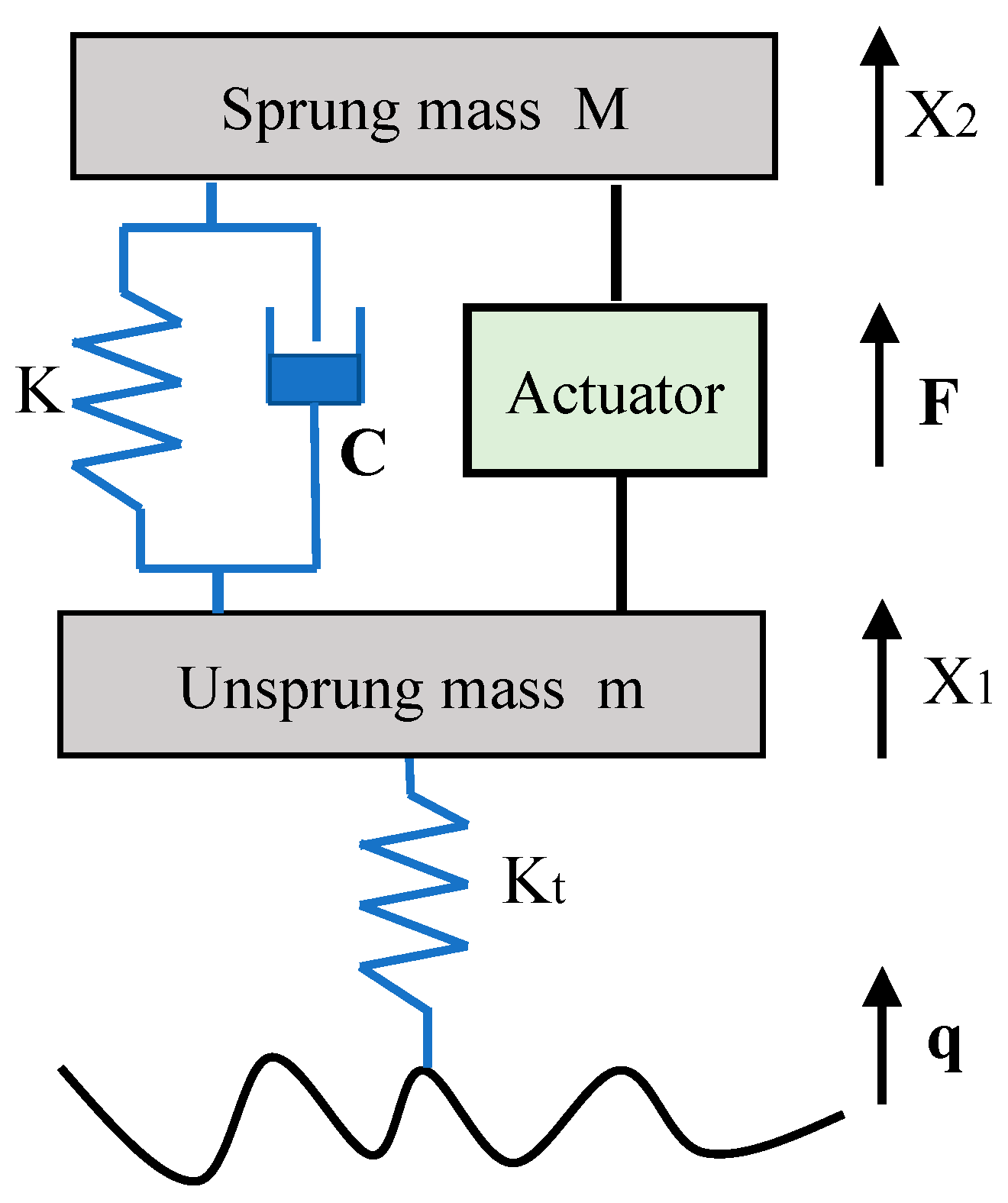
Figure 1. The vehicle model.
Machines 13 00983 g001
Figure 2. The residual policy learning framework.
Machines 13 00983 g002
Figure 3. The structure of the actor neural network.
Machines 13 00983 g003
Figure 4. The structure of the critic neural network.
Machines 13 00983 g004
Figure 5. The training process using the improved TD3 method.
Machines 13 00983 g005
Figure 6. The road excitation of a class B road.
Machines 13 00983 g006
Figure 7. The body acceleration of a class B road.
Machines 13 00983 g007
Figure 8. The body displacement of the class B road.
Machines 13 00983 g008
Figure 9. The body velocity of the class B road.
Machines 13 00983 g009
Figure 10. The RRL output of the class B road.
Machines 13 00983 g010
Figure 11. The road excitation of the Class E road.
Machines 13 00983 g011
Figure 12. The body acceleration of the class E road.
Machines 13 00983 g012
Figure 13. The body displacement of the Class E road.
Machines 13 00983 g013
Figure 14. The body velocity of the Class E road.
Machines 13 00983 g014
Figure 15. The RRL output of the class E road.
Machines 13 00983 g015
Table 1. Road roughness values.
Road ClassLower LimitGeometric MeanUpper Limit
A-16 × 10−6 32 × 10−6
B32 × 10−6 64 × 10−6 128 × 10−6
C128 × 10−6 256 × 10−6 512 × 10−6
D512 × 10−6 1024 × 10−6 2048 × 10−6
E2048 × 10−6 4096 × 10−6 8192 × 10−6
Table 2. The parameters of the RRL method.
DefinitionItemValues
CriticLearnRate5 × 10−5
GradientThreshold1
ActorLearnRate1 × 10−4
GradientThreshold1
AgentSampleTime0.01
TargetSmoothFactor1 × 10−3
DiscountFactor0.95
MiniBatchSize128
ExperienceBufferLength1 × 106
TargetUpdateFrequency10
MaxEpisodes500
LQR K ˜ 2.03 × 10 4 , 4.61 × 10 2 , 4.44 × 10 3 , 9.74 × 10 2
Table 3. The parameters of the suspension.
SymbolValues
m 43   kg
M 365   kg
C 1000   N s / m
K 24,000   N / m
K t 35,000   N / m
Table 4. The RMS of the suspension control on the class B road.
MethodsBody AccelerationBody DisplacementBody Velocity
Passive1.53390.00530.0453
LQR1.3256 (13.5824%)0.0050 (5.6603%)0.0254 (43.914%)
TD31.2846 (16.2544%)0.0047 (11.3207%)0.0209 (53.9503%)
RRL1.0994 (28.3286%)0.0046 (13.1371%)0.0179 (60.4617%)
Table 5. The RMS of the suspension control on the class E road.
MethodsBody AccelerationBody DisplacementBody Velocity
Passive3.26550.02390.1485
LQR2.8384 (13.08%)0.0148 (37.9345%)0.0720 (51.5134%)
TD32.7677 (15.2438%)0.0147 (38.6219%)0.0507 (65.834%)
RRL2.2336 (31.5988%)0.0136 (43.2449%)0.0472 (68.1833%)
Disclaimer/Publisher’s Note: The statements, opinions and data contained in all publications are solely those of the individual author(s) and contributor(s) and not of MDPI and/or the editor(s). MDPI and/or the editor(s) disclaim responsibility for any injury to people or property resulting from any ideas, methods, instructions or products referred to in the content.