Economy Optimization by Multi-Strategy Improved Whale Optimization Algorithm Based on User Driving Cycle Construction for Hybrid Electric Vehicles

Abstract

Nowadays, there is an increasing focus on enhancing the economy of hybrid electric vehicles (HEVs). This study builds a framework model for the parameter optimization of hybrid powertrains in user driving cycles. Unlike the optimization under standard driving cycles, the applied user driving cycle incarnates realistic driving situations, and the optimization results are more realistic. Firstly, the user driving cycle with high accuracy is constructed based on actual driving data, which provides a basis for the performance analysis of HEV. Secondly, the HEV model with good power and economy is constructed under user driving cycles. Finally, a multi-strategy improved whale optimization algorithm (MIWOA) is proposed, which can guarantee better economy of HEV compared with the original whale optimization algorithm (WOA). The economy optimization of HEV is completed by MIWOA under user driving cycles, and the hybrid vehicle economy parameters that are more in line with the user’s actual driving conditions are obtained. After optimization, the 100 km equivalent fuel consumption (EFC) of HEV is reduced by 5.20%, which effectively improves the vehicle’s economy. This study demonstrates the effectiveness of the MIWOA method in improving economy and contributes a fresh thought and method for the economic optimization of the hybrid powertrain.

1. Introduction

As automobile fuel consumption (FC) and emission regulations become more and more stringent [1], it is difficult for traditional fuel vehicles to meet the limited standards. HEVs have become a key topic [2] in the field of automobile research by virtue of their advantages of good power performance [3], good fuel economy [4], multiple power sources [5], and low emissions [6]. The driving cycle is a crucial criterion for hybrid vehicle product design and development [7], powertrain system design [8], performance evaluation [9], and economic optimization [10]. Due to the differences in vehicle models and application scenarios, the driving conditions of hybrid vehicles vary greatly. However, the existing standard driving cycles are not representative of actual application scenarios and are difficult to meet user needs [11]. Therefore, it is particularly important to gather the traveling data of users of the same hybrid vehicle model and construct a driving cycle that covers the user’s usage as much as possible [12].

Currently, the economic evaluation of hybrid vehicles is mainly carried out under standard driving conditions, without fully considering the real-world driving conditions [13]. Therefore, constructing representative user driving cycles can offer a more valuable basis for vehicle economy analysis [14]. In addition, the hybrid powertrain parameters significantly affect the economy of the whole vehicle [15], so it is essential to develop driving cycles based on user data and explore methods that can be used to optimize hybrid powertrain parameters [16].

1.1. Literature Review of Driving Cycles

Driving cycles are mainly divided into two categories: modal and transient [17,18]. Transient driving cycles are generated based on the actual road driving data of the vehicle [19], which involves a lot of velocity variations and is in accord with the real driving scene. Similarly, transient driving cycles are the mainstream direction of the current driving cycle’s construction. The generated driving cycle based on user traveling data in this paper also belongs to transient conditions. For the development of transient driving cycles, the commonly used methods are based on the Markov chain method and cluster analysis [14]. Ma et al. used the Markov chain method to construct a driving cycle that was closer to the real driving conditions with the GPS trajectory data of 459 cars [20]. Zhang et al. proposed a new type of Markov chain evolution algorithm, which improved the Markov chain evolutionary algorithm by combining random sampling and evolutionary algorithms to improve the efficiency of Markov chains [21]. Nyberg et al. used the Markov chain method to achieve a compressed database and efficient feature variables, generated candidate driving conditions, and converted the candidate set into equivalent driving cycles [22].

Using the Markov chain method requires state partitioning but the partitioning method is rough [23]. For this reason, there are many scholars who use clustering algorithms and other methods to divide the states first and then complete the construction of driving conditions based on Markov chain theory, which effectively suppresses the impact of Markov randomness on the accuracy of the constructed driving conditions. Brady et al. used neural networks to classify the dataset and generated a driving cycle based on Markov process theory, which provided a more accurate basis for electric vehicle development and powertrain design [9]. Zhao et al. used K-means and support vector machine hybrid algorithms to divide kinematic fragments and constructed a driving cycle based on Markov and Monte Carlo simulation methods by using the relative error, performance value, and velocity–acceleration probability distribution as decision criteria [24].

However, if the Markov chain theory is adopted, the problems of excessive computation, long overall time consuming, and low efficiency of driving cycle construction due to randomness still exist. Therefore, many scholars have adopted cluster analysis to develop transient driving cycles. Berzi et al. pre-processed the collected data and then used the k-means algorithm to complete the grouping of eligible micro-trips and finally constructed ten different driving cycles for five vehicle classes [7]. Yang et al. used principal component analysis (PCA) and K-means clustering to construct two driving cycles for passenger cars in Nanjing in 2009 and 2017 [25]. Omar et al. developed two global driving cycles based on a huge and various database using K-means and K-medoids clustering methods, which were the first vehicle driving cycles in the Greater Cairo region of Egypt [26]. Wang et al. used PCA and clustering algorithm to identify operating segments and obtained five typical operating conditions by extracting the operating segments and characteristic parameters related to the dominant failure loads of the electric drive system [27]. Tang et al. developed typical driving cycles using PCA and clustering analysis [28]. Obviously, the final generated driving cycles faithfully reflect the actual driving characteristics.

1.2. Literature Review on Economic Optimization of Hybrid Powertrains

The hybrid powertrain mainly includes the engine, electric motor, battery, transmission, main reducer, and controller [29], and their related parameters have a large impact on the economy of hybrid vehicles [30,31]. Optimizing hybrid powertrain parameters is generally considered from two aspects: component parameters and control parameters. For optimization problems in automotive engineering, meta-heuristic algorithms are frequently used by various researchers [32]. For the optimization of hybrid powertrain component parameters, Lei et al. used non-dominated sorting genetic algorithm-II to optimize the transmission ratio of the hybrid powertrain with the goal of optimizing engine FC and battery loss, which reduced FC and battery capacity loss [11]. For the optimization of control parameters of hybrid vehicles, Jeoung et al. proposed an optimal shift strategy based on the greedy control method of speed prediction, which improved fuel efficiency [33]. Zhang et al. combined the dynamic objective with the economic objective and optimized the shift law by using a particle swarm algorithm, and the ultimate shift schedule improved the dynamics and economy in an integrated way [34].

However, both component parameters and control parameters of the powertrains affect vehicles’ economies, so this study considers optimizing the above two types of parameters at the same time. Eckert et al. took engine FC, pollutant emission, and transmission mechanical loss as the optimization objectives, and used an interactive adaptive weight genetic algorithm (GA) to search for the optimal vehicle drive-line design scheme and gearshift control strategy, and the results showed that the parameters in the optimization objectives all achieved significant improvement [35].

Through the above analysis, the adoption of valid optimization algorithms is the essential point to improve the economy of HEVs. Most researchers currently use GA, particle swarm optimization, or their improved algorithms to complete the parameter optimization work, and the methods used are relatively traditional. Generally, these methods use a random method to generate the initial population, which is pseudo-random; the search method is relatively single, and the optimization result easily falls into the local optimum. Thus, it is especially important to propose more effective optimization methods. In addition, due to many parameters of the hybrid powertrain, it is difficult to consider all the parameters in the economic optimization study. With the different driving cycles, the transmission ratio [36,37] and gearshift moment of the hybrid powertrain need to be adjusted accordingly. Therefore, this paper proposes a new MIWOA method to carry out the economy optimization of hybrid vehicles starting from optimizing the main reduction ratio and shift schedule.

1.3. Main Contributions and Structure of Article

After the discussion in Section 1.1, both the Markov chain and the cluster analysis method can construct the driving cycle with a good accuracy, but the construction efficiency of the cluster analysis method is higher than that of the Markov chain method. Also, in the context of big data, the method of constructing driving cycles with high accuracy and less computation is favored by various researchers [38]. Thus, this paper constructs a user driving cycle adopting a cluster analysis method and designs a hybrid powertrain parameter optimization model under this driving cycle. The results of the study provide manufacturers with a basis for developing vehicles with driving cycles that are closer to the realistic driving conditions of users. Meanwhile, this paper contributes a new method of hybrid powertrain parameter optimization based on the user driving cycle to improve vehicle economy, which solves the problem of difficult optimization of hybrid system parameters. The primary work and contributions of this study are as follows:

• Select feature parameters oriented to average instantaneous fuel consumption characteristics. This research applies the stepwise regression method to complete the selection of characteristic parameters oriented to the average instantaneous fuel consumption characteristics, which addresses the problem of high randomness in the selection of eigenvalues and provides a guarantee for the clustering effect.
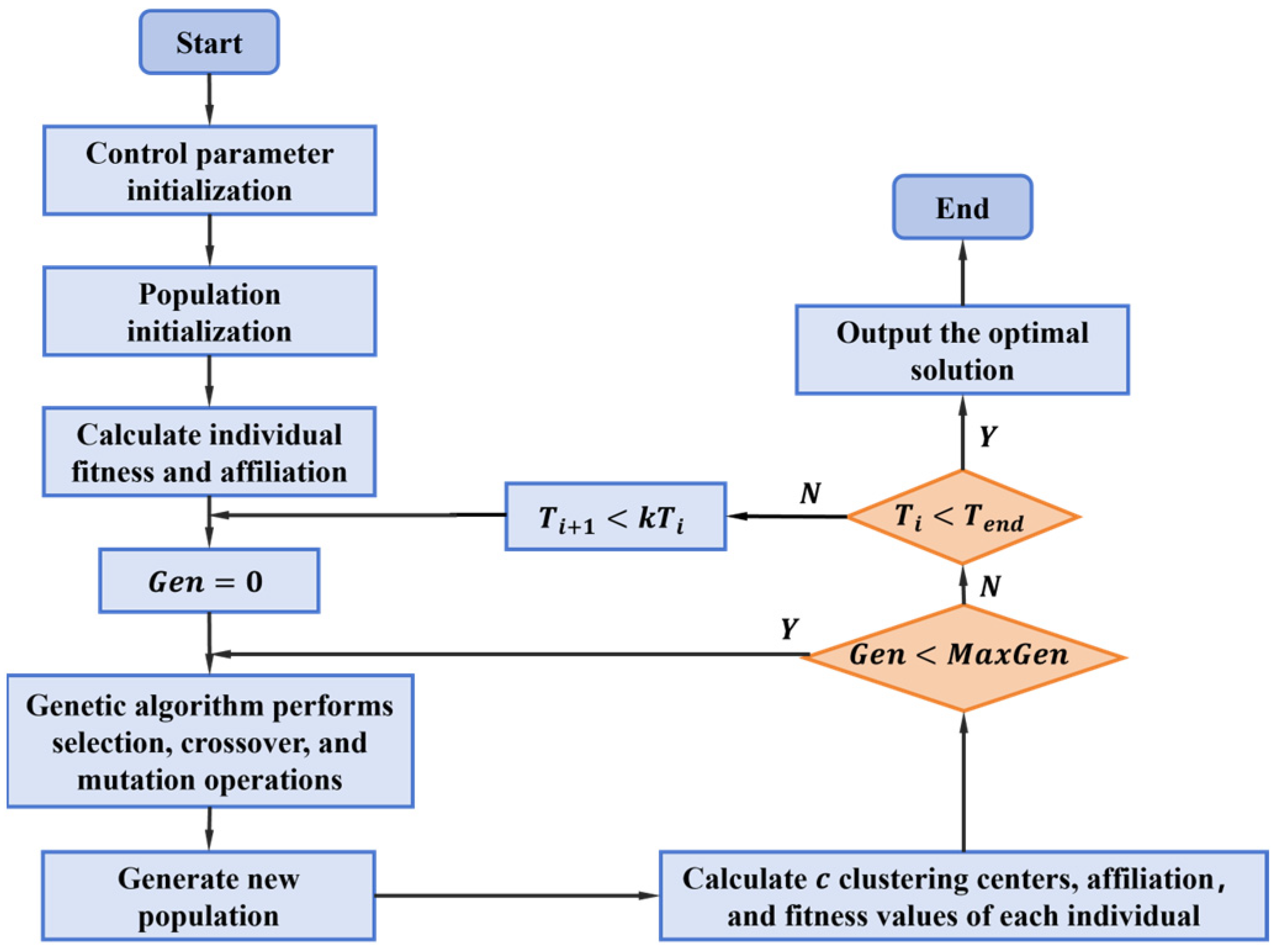
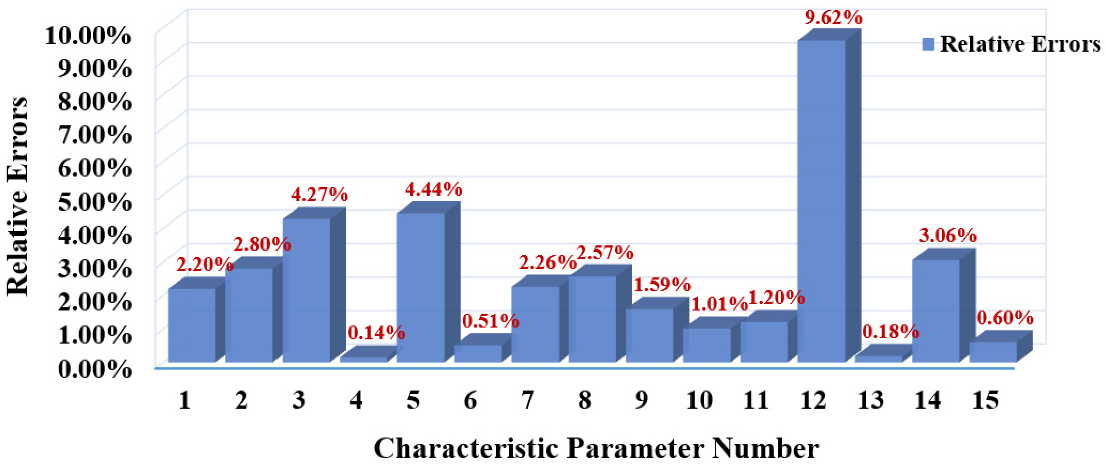
• The simulated annealing genetic algorithm fuzzy c-means clustering (SAGAFCM) methodology is employed to develop the user driving cycle. This method overcomes the problem that FCM is susceptible to the initial clustering center and converges to a local minimal point and thus improves the reliability of the clustering results. The average deviation of the 15 eigenvalues of the constructed conditions is 2.4313%, which is a high accuracy.
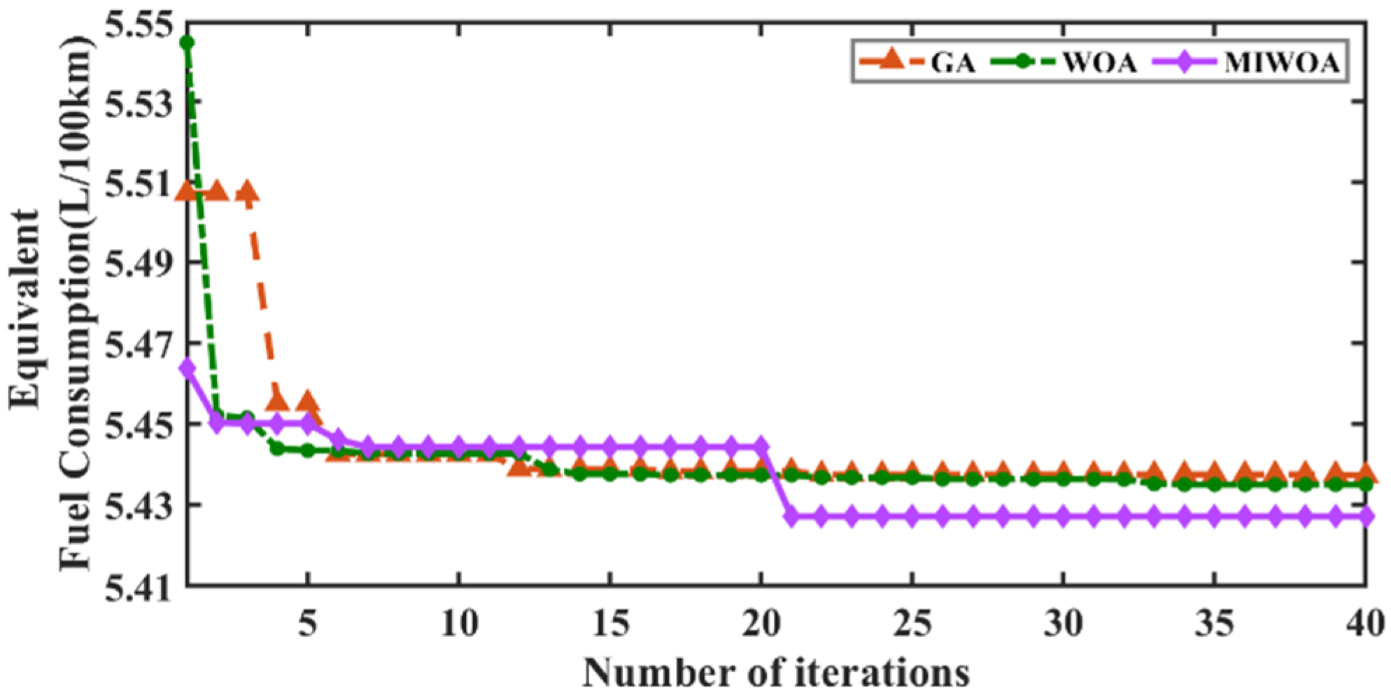
• This study proposes the MIWOA method to optimize the component parameters and control parameters of the hybrid powertrain under user driving cycles. The combination of Fuch and opposition-based learning (OBL) enhances the diversity of the initial population, which solves the problem of pseudo-randomness of the initial population generated by the random method of the original algorithm; the proposed variable spiral parameter enriches the search of whales and improves the ability of the algorithm to explore globally; and the adaptive weights are combined with t-distribution perturbation and random perturbation, respectively, to improve the likelihood of jumping out of the local optimum. Thus, the economic parameters of HEVs that are more in line with the user’s actual driving conditions are obtained, and the vehicle’s economy is enhanced.

The other sections of this paper are composed as follows: Section 2 introduces the construction of the model framework and user driving cycle; Section 3 introduces the basic information of the model and verifies its reasonableness; Section 4, based on the user driving cycle, completes the optimization of the hybrid powertrain component parameters and control parameters by using the proposed MIWOA method; and Section 5 concludes the primary work of this research.

2. Model Framework Development and Driving Cycle Construction

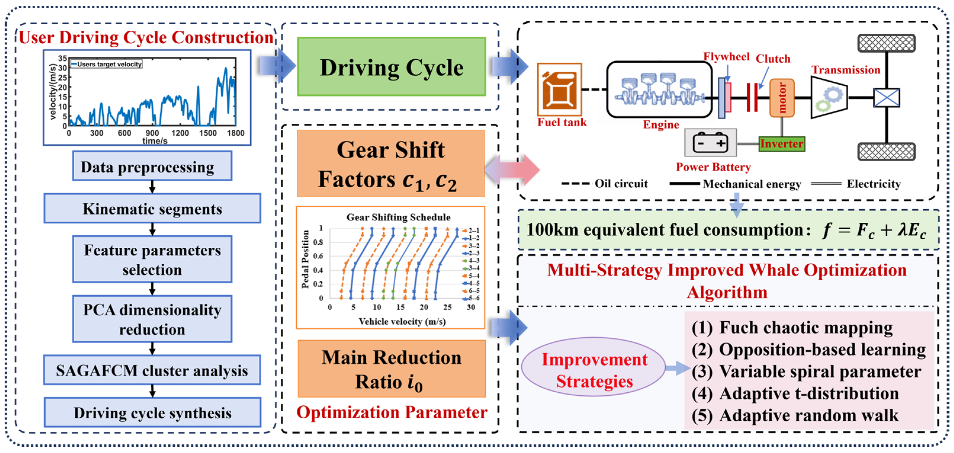
2.1. Overview of Model Framework

This section describes the procedure of establishing a model framework for optimization of hybrid powertrain parameters based on user driving cycles and details the process of user driving cycle construction. The model framework is shown in Figure 1, which includes three main modules.

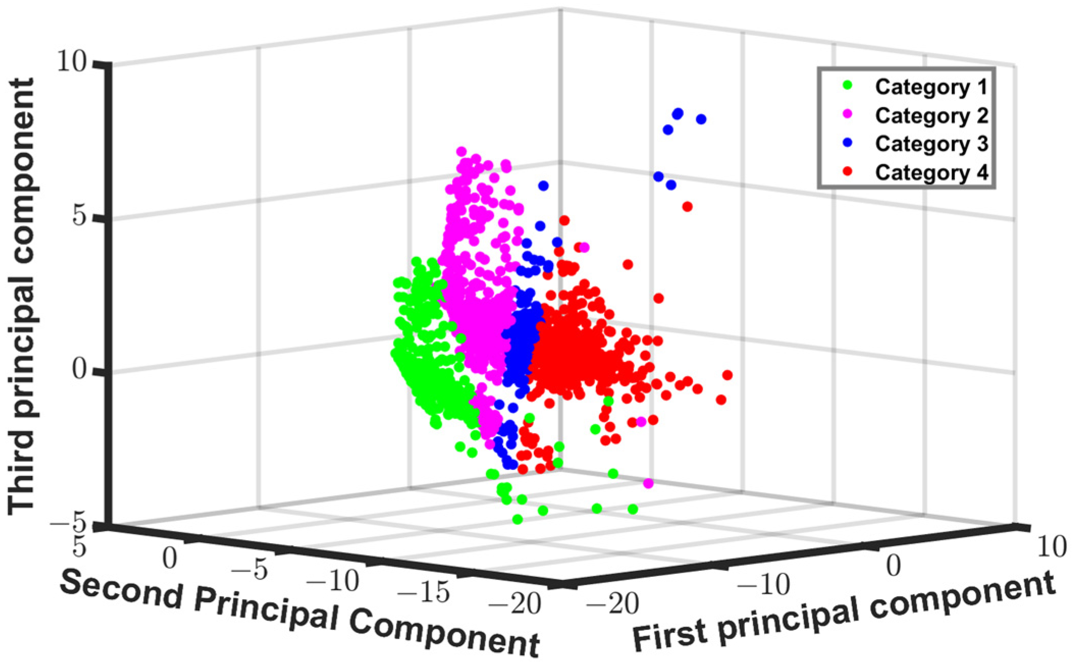
• Driving cycle module: Based on the Vehicle Network Data, the kinematic segments are categorized using PCA and the SAGAFCM algorithm. Depending on the percentage of overall time accounted for by each type of kinematic segment, appropriate kinematic segments are selected from each category and together connected to synthesize user driving cycle that meets the features of the user database.
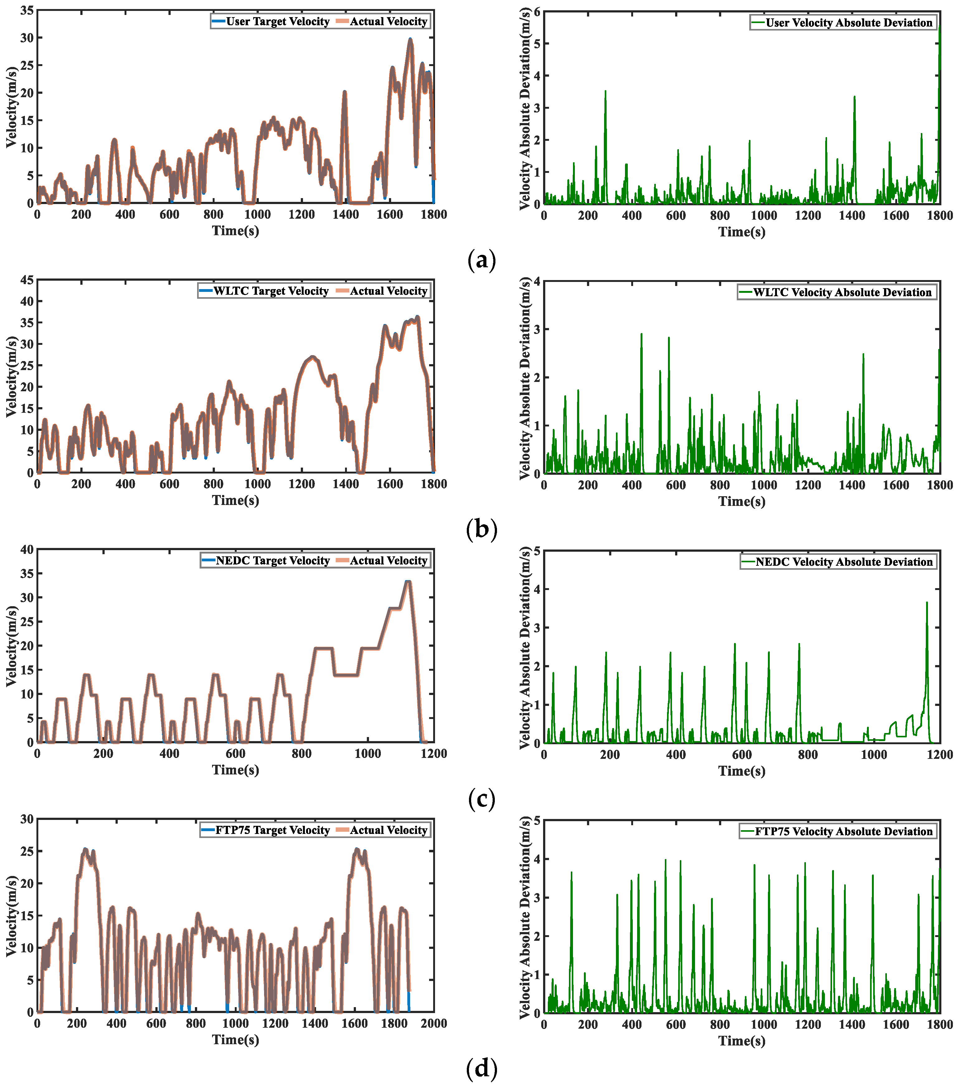
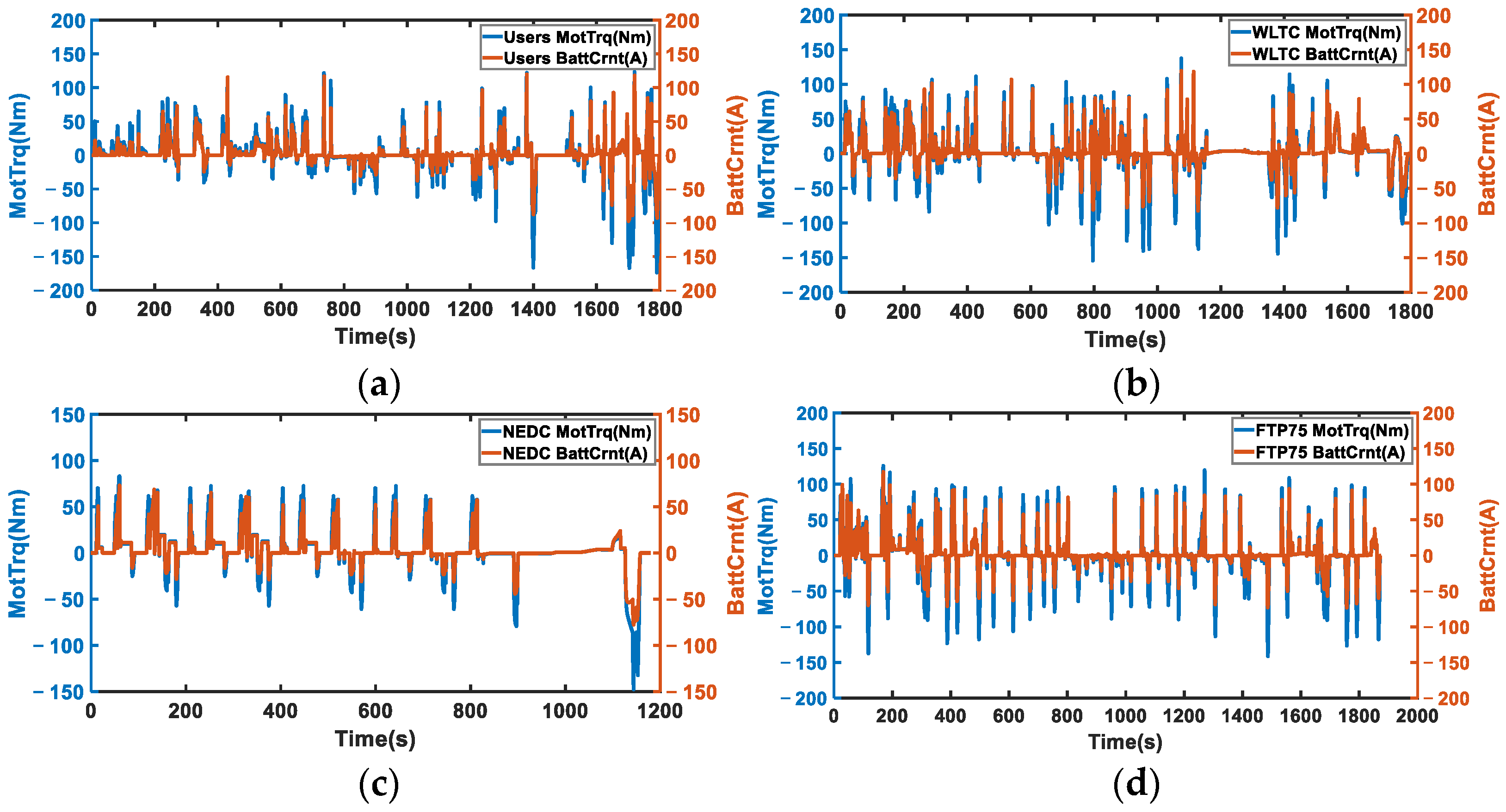
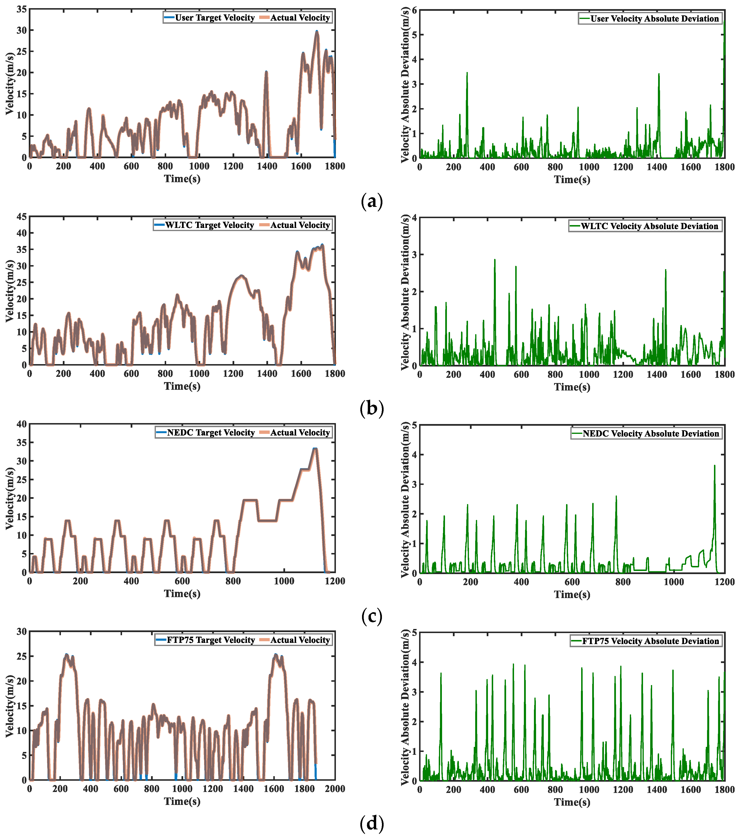
• Hybrid vehicle model: Under the user driving cycle, an HEV model of P2 configuration is built based on the rule-based strategy, which is required to fulfill power requirements of the user driving cycle and has good economy. Meanwhile, the model is verified under other standard driving cycles to ensure the rationality of the model. In fact, the vehicle needs to meet the driving requirements not only for the user driving cycle, but also for the standard driving cycles, so the model simulation verification is operated under the other three standard driving cycles to ensure the used model’s rationality.
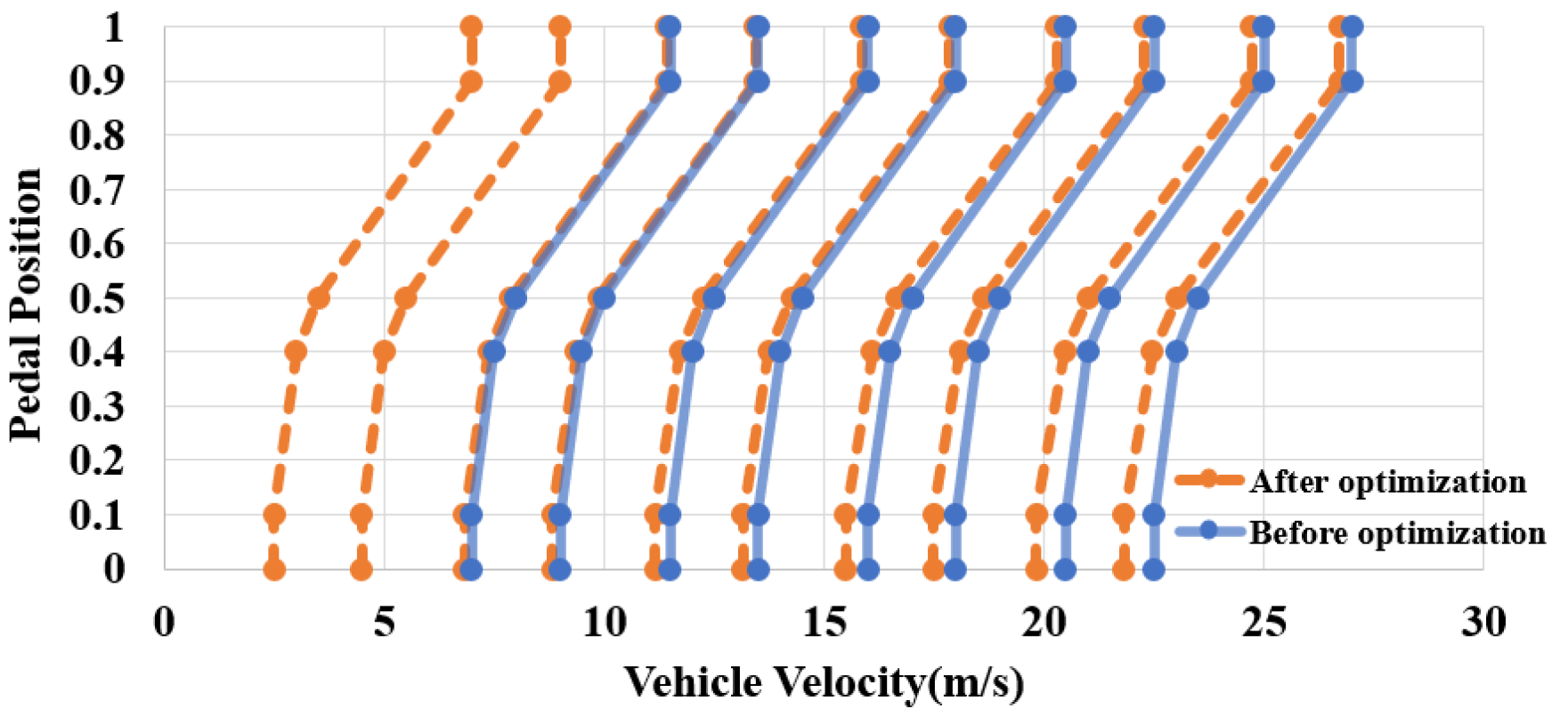
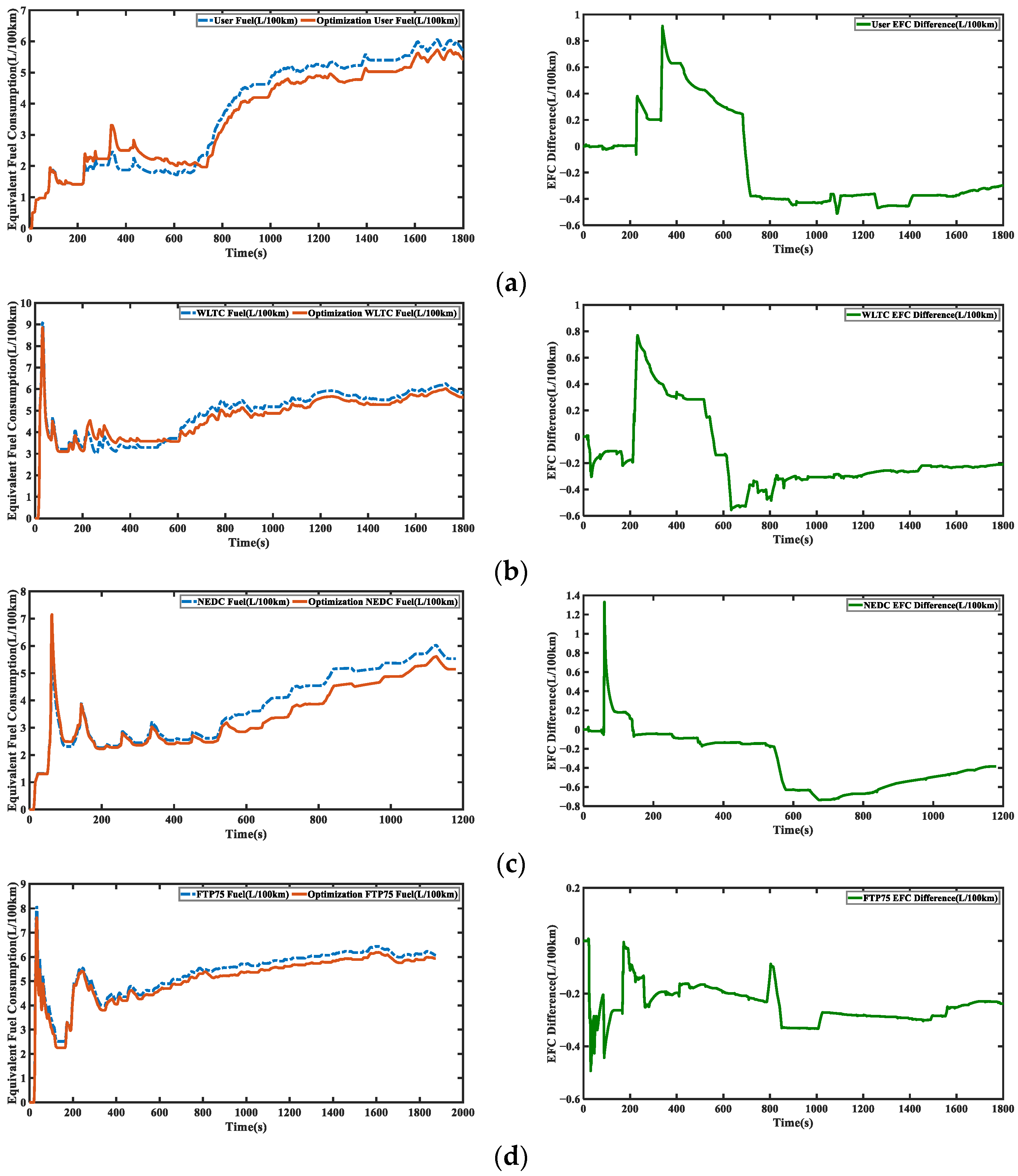
• MIWOA optimization module: To comprehensively consider the economy of HEVs, the FC of the engine and the energy consumption of the battery are transformed into 100 km EFC. Based on the HEV model of user driving cycles, with 100 km EFC as the optimization objective function and the main reduction ratio and gear shift factors as the optimization variables, MIWOA is proposed to complete the economic optimization of the hybrid vehicle under the constraints, and then this paper compares the simulation results of the model before and after optimization. Meanwhile, the driving requirements of standard driving cycles should be considered, so the simulation results before and after optimization are compared under other standard driving cycles, which proves the effectiveness of the optimization method proposed in this paper.

2.2. Construction of User Driving Cycle

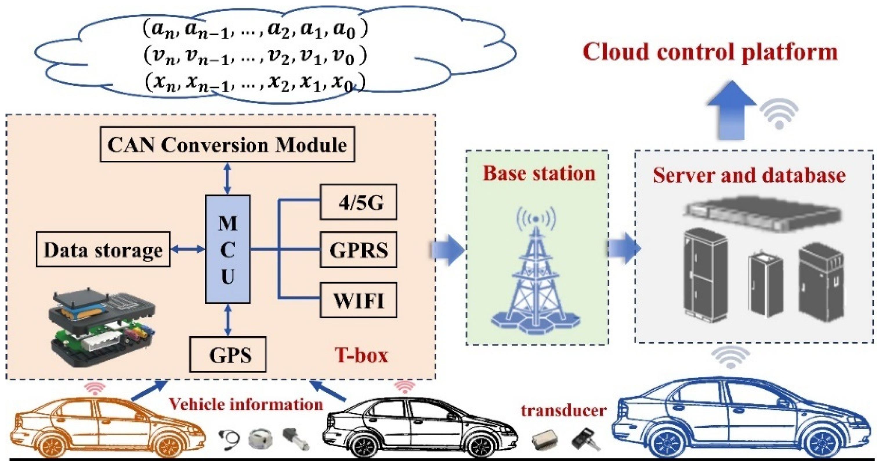
2.2.1. Data Sources

The gathered data need to incarnate the actual driving specificities of the users as much as possible, so the research adopts a natural driving mode for users of the same hybrid model and collects users’ driving data through the Internet of Vehicles system. The data collection principle is shown in Figure 2. The vehicles are equipped with telematics box (T-box) devices and a variety of sensors, including velocity sensors, three-dimensional acceleration sensors and more. The sensors are mainly responsible for collecting vehicle information. The T-box can realize communication with the CAN bus through the CAN conversion module, so that it can obtain data information such as time, velocity, hybrid powertrain, and control system. Simultaneously, T-box can obtain the location information of the vehicle and the surrounding environment through the Global Positioning System (GPS) module. Finally, T-box converts serial communication into wireless communication through its built-in General Packet Radio Service (GPRS) module, realizes its communication with base stations and roadside units, and then uploads the acquired data to the cloud control platform to achieve the purpose of data interaction between the user layer and the cloud server.

The actual driving data of the same hybrid vehicle model, which contain multiple users and covers different regions, are the fundamental basis for constructing the driving conditions of users. With the development of intelligent connected cars, the interaction of various types of information becomes more and more convenient [39]. Therefore, this study only collects the driving data under normal driving conditions without additional experiments and tests, which greatly simplifies the procedure of data acquisition and eases the workload of data acquisition. In this paper, actual driving data covering users of the same model in different regions are collected based on the big data platform of SAIC-GM-Wuling Automobile Co., Ltd. (Liuzhou, China), mainly including time, velocity, engine speed and torque, instantaneous fuel consumption, accelerator pedal opening, battery voltage, battery current, generator speed, motor speed, power battery power, etc., and the frequency of data acquisition is 1 Hz. They cover 84 hybrid vehicles of the same model, covering driving areas including Beijing, Shanghai, Shaanxi, Jiangxi and Shandong provinces, and other regions, with a cumulative volume of 660,000 pieces of data. The data used in the research involve many vehicles, a wide geographic distribution, and a large difference in the traffic situation in various places, so the representativeness of the data is obvious, which have certain research value.

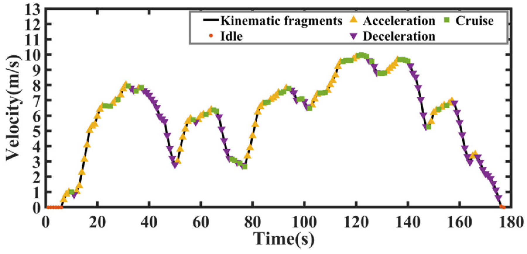
2.2.2. Data Pre-Processing and Establishment of Kinematic Fragment Library

The bad data mainly include several types of duplicate data, outliers, time discontinuity, and long-term parking data. Among them, duplicate data and outliers are directly deleted during the data pre-processing phase. For discontinuous data, if the time interval is greater than or equal to 4 s, the dataset is directly separated from here, and it will be used as the starting point of a new data fragment. Most researchers would choose to delete the discontinuous data directly, but the treatment in this paper can improve the utilization of data and help to ensure the accuracy of the data. If the time interval of the data is equal to 2 or 3 s, the data generally do not undergo sudden changes due to the short time interval. Because linear interpolation is simple, convenient, and operable, this paper chooses to use linear interpolation to make up for the missing data.

The processed data are labeled into four states, namely, idle, acceleration, deceleration, and cruise, according to the rules in

Table 1. Principle of kinematic segment division.

Indicator	Idle	Acceleration	Deceleration	Cruise
Velocity (km/h)	<1	≥1	≥1	≥1
Acceleration (m/s2)	-	>0.1	<−0.1	≥−0.1 & ≤0.1

. The kinematic segment that extracts the velocity starting from 0 and contains the above four states of motion until the velocity is 0 again, is shown in Figure 3. Among them, if the velocity is 0 for more than 180 s, it is considered that the bad data of long-term parking occurs, and it is excluded when dividing the kinematic segments. According to the above rules, a total of 1842 kinematic segments were finally obtained.

2.2.3. Selection of Feature Parameters

The eigenvalues involved in clustering [40] have a large impact on the clustering effect. However, there is no uniform standard for the selection of feature parameters, which is easy to cause the problem of redundancy or too strong randomness of feature parameters. Aiming at the above problems, this study adopts the stepwise regression method [40] to carry out the selection of feature parameters oriented to average instantaneous fuel consumption characteristics. The steps are listed below.

• Dependent variable: First calculate the average instantaneous FC of each kinematic segment.
• Independent variable: Select and calculate the initial parameters of the kinematic segments, including 50 variables such as average velocity, average acceleration, standard deviation of velocity, average engine speed, etc.
• Establish a linear regression model of 50 feature parameters and average instantaneous FC.

$$\widehat{y}={\beta }_0+{\beta }_1{x}_1+{\beta }_2{x}_2+{\beta }_3{x}_3+\dots +{\beta }_n{x}_n+\epsilon$$

(1)

where $\widehat{y}$ denotes the regressed average instantaneous FC value, ${\beta }_0$ is the regression constant, ${\beta }_1$, ${\beta }_2$, ${\beta }_3$,…, ${\beta }_n$ denote the regression coefficient of n feature parameters, and $x_1$, $x_2$, $x_3$,…, $x_n$ denote the feature parameters of each kinematic segment.

To explore the link between the feature parameters and the average instantaneous FC, the effect of regression is examined by the sum value at the significance level of 0.05. Finally, R-squared is 0.925 and the adjusted R-squared is 0.9239, both of which are closer to 1 and p = 0. From this, it can be judged that the fit is better and the regression model is more accurate. Moreover, 27 variables are retained in the final model, which means that these 27 variables have a high correlation with the average instantaneous FC, as shown in

Table 2. Eigenvalues linearly correlated with average instantaneous FC.

No.	Feature Parameters	No.	Feature Parameters
1	$\mathrm{Idle} \mathrm{time} (\mathrm{s}$)	15	$\mathrm{Standard} \mathrm{deviation} \mathrm{of} \mathrm{engine} \mathrm{speed} (\mathrm{r}\mathrm{p}\mathrm{m}$)
2	$\mathrm{Deceleration} \mathrm{time} (\mathrm{s}$)	16	$\mathrm{Minimum} \mathrm{engine} \mathrm{speed} (\mathrm{r}\mathrm{p}\mathrm{m}$)
3	$\mathrm{Average} \mathrm{velocity} (\mathrm{m}/\mathrm{s}$)	17	$\mathrm{Maximum} \mathrm{engine} \mathrm{speed} (\mathrm{r}\mathrm{p}\mathrm{m}$)
4	$\mathrm{Velocity} \mathrm{standard} \mathrm{deviation} (\mathrm{m}/\mathrm{s}$)	18	$\mathrm{Standard} \mathrm{deviation} \mathrm{of} \mathrm{motor} \mathrm{speed} (\mathrm{r}\mathrm{p}\mathrm{m}$)
5	$\mathrm{Maximum} \mathrm{acceleration} (\mathrm{m}/{\mathrm{s}}^2$)	19	$\mathrm{Minimum} \mathrm{motor} \mathrm{speed} (\mathrm{r}\mathrm{p}\mathrm{m}$)
6	$\mathrm{Average} \mathrm{engine} \mathrm{speed} (\mathrm{r}\mathrm{p}\mathrm{m}$)	20	$\mathrm{Standard} \mathrm{deviation} \mathrm{of} \mathrm{engine} \mathrm{torque} (\mathrm{N}\mathrm{m}$)
7	Average pedal opening (%)	21	$\mathrm{Minimum} \mathrm{engine} \mathrm{torque} (\mathrm{N}\mathrm{m}$)
8	$\mathrm{Average} \mathrm{motor} \mathrm{speed} (\mathrm{r}\mathrm{p}\mathrm{m}$)	22	$\mathrm{Maximum} \mathrm{motor} \mathrm{torque} (\mathrm{N}\mathrm{m}$)
9	$\mathrm{Average} \mathrm{motor} \mathrm{torque} (\mathrm{N}\mathrm{m}$)	23	$\mathrm{Maximum} \mathrm{voltage} (\mathrm{V}$)
10	$\mathrm{Velocity} 0–10 \mathrm{k}\mathrm{m}/\mathrm{h}$ time ratio	24	$\mathrm{Maximum} \mathrm{current} (\mathrm{A}$)
11	$\mathrm{Velocity} 30–40 \mathrm{k}\mathrm{m}/\mathrm{h}$ time ratio	25	$\mathrm{Average} \mathrm{current} (\mathrm{A}$)
12	$\mathrm{Velocity} 40–50 \mathrm{k}\mathrm{m}/\mathrm{h}$ time ratio	26	Maximum state of charge (SOC) (%)
13	$\mathrm{Velocity} 70–80 \mathrm{k}\mathrm{m}/\mathrm{h}$ time ratio	27	Average SOC (%)
14	$\mathrm{Velocity} > 90 \mathrm{k}\mathrm{m}/\mathrm{h}$ time ratio

.

2.2.4. Data Dimensionality Reduction

Twenty-seven characteristic parameters significantly related to average instantaneous fuel consumption are identified by a stepwise regression method, but the clustering efficiency is low because of the large number of variables. Therefore, this study firstly considers to decline the variables’ dimensionalities by PCA before clustering analysis. However, due to the different units of each feature parameter, this paper standardizes the feature parameters to unite the proportion of each characteristic parameter in the feature data space. Subsequently, the standardized 27 sets of eigenvalues are then used as the original variables to further carry out PCA. As shown in Figure 4, the sum of the contribution rates of the first eight columns of values among them is 86.02% after PCA, which demonstrates that the first eight columns of values can replace most variations in the data space and can represent the overall characteristics of the feature parameters. Therefore, in the following work, the scores of the first eight principal components are used as the principal components corresponding to the eigenvalues to participate in the cluster analysis, and their component scores are shown in

Table 3. Source of first eight principal components.

No.	1st	2nd	3rd	4th	5th	6th	7th	8th
1	−15.17	−17.79	−0.423	0.39	−1.69	−2.00	−1.17	−0.09
2	−18.04	−15.30	−2.72	0.60	−0.63	−0.60	0.06	−0.05
3	−14.76	−18.18	0.50	0.59	−0.83	−2.65	−1.07	0.37
4	−17.43	−16.05	−0.05	0.77	−0.83	−1.55	−0.69	−0.38
5	−18.14	−15.22	−2.50	0.17	−0.92	−0.32	−0.13	−0.002
6	−13.62	−19.03	−0.18	−0.62	−1.64	−3.02	−0.86	0.42
…
1841	2.47	−1.57	2.59	−0.56	0.25	−1.68	−0.32	0.20
1842	3.11	−1.25	−0.61	−1.27	−0.25	−0.64	−0.36	0.15

.

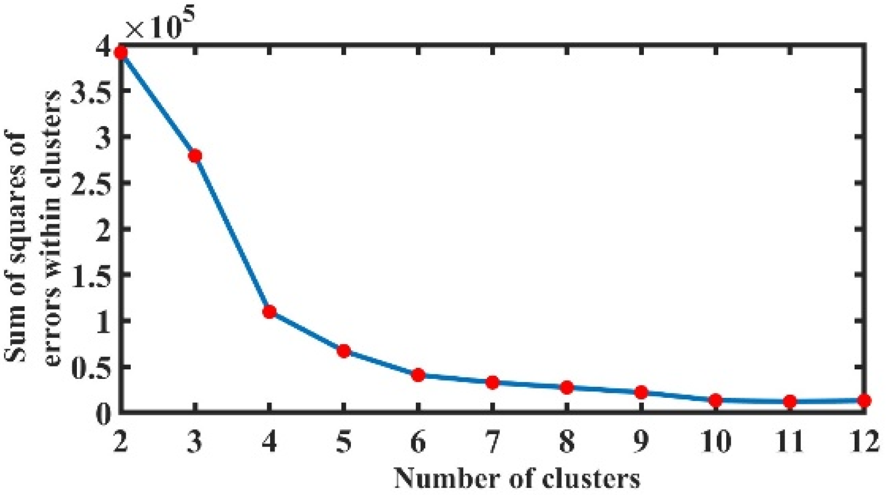
2.2.5. SAGAFCM Cluster Analysis

Cluster analysis methods play an important role in the big data mining processing. When using the clustering algorithm, the setting of the number of clusters N is very important. The methods of determining N values are generally based on practical needs, the elbow rule, the contour coefficient method, etc. In real life, the driving conditions of vehicles are generally divided into three or four categories, so from the perspective of practical needs, the number of clusters should be selected three or four. In addition, Figure 5 shows the mean square error curve of the clustered data with different values of N. The elbow point is at the position of N = 4, so the clustering result is optimal when N is equal to 4. Therefore, on the basis of combining practical needs and elbow law, the final number of clusters is determined to be four in this paper.

The FCM algorithm is a local search optimization algorithm whose performance is easily affected by the initial clustering center. If the initial clustering center is not properly selected, it is very easy to converge to a local minimal point. And even if the algorithm is applied under the same conditions, the randomness of the clustering center selection will still lead to inconsistent clustering results, which affects the precision of driving cycle construction. Accordingly, the method of SAGA can optimize the primary clustering centers to acquire the optimal primary clustering centers [41]. In addition, the combination of a simulated annealing algorithm and GA effectively avoids the problem of premature maturity of GA [41,42]. Therefore, SAGAFCM can prevent premature convergence while adjusting and optimizing the population, further improving the reliability of the clustering results. Figure 6 shows the flowchart of SAGAFCM.

In accordance with the above principles and based on the previously determined number of clustering clusters, the score data of principal component in Table 3 are clustered, and the dataset is finally classified into four categories. To observe the classification effect more intuitively, Figure 7 illustrates the sample scatter plot for the first three principal components. It demonstrates that the boundaries of the four categories of data are clearer and the categorization is more effective.

2.2.6. Synthesis of User Driving Cycles

To accurately reflect the user’s actual driving conditions, a certain percentage of segments from each category after clustering need to be extracted for fitting. Calculations show that the percentage of total time for categories 1, 2, 3, and 4 is 10%, 19%, 12%, and 59%, respectively. According to the above proportion, appropriate kinematic segments are selected from the four categories, respectively, and combined in turn. Figure 8 shows the final synthesized user driving cycle with a total duration of 1800 s.

To check whether the constructed user driving cycle is close to the pre-processed dataset, the relative errors of the 15 feature parameters with the dataset are contrasted, as shown in

Table 4. Characterization indicators.

No.	Characteristic Parameters	No.	Characteristic Parameters
1	Average velocity	9	Acceleration time ratio
2	Average traveling velocity	10	Deceleration time ratio
3	Standard deviation of velocity	11	Cruise time ratio
4	Average acceleration of acceleration section	12	Maximum velocity
5	Standard deviation of acceleration	13	Average engine speed
6	Average deceleration	14	Maximum voltage
7	Standard deviation of deceleration	15	Average voltage
8	Idle time ratio

and Figure 9. Among the 15 eigenvalues, except for the error of the maximum velocity, which is 9.62%, the errors of the remaining 14 eigenvalues are less than 4.5%. Also, the average error of the eigenvalues is 2.4313%, which is much smaller than the 5% threshold adopted by many researchers. To sum up, the overall error of the developed user driving condition is smaller and more stable, and the effect is better. The maximum velocity belongs to the extreme value, and its larger error is also a normal phenomenon, but its error is still smaller than the 10% threshold chosen by many researchers. Hence, this paper considers that the maximum velocity error is still within the acceptable range. Therefore, the generated driving cycle using the SAGAFCM method can faithfully incarnate the whole feature and serve as a benchmark for the following optimization of hybrid powertrain parameters.

3. Model and Simulation

3.1. Basic Information of Model

3.1.1. HEV Dynamics Model

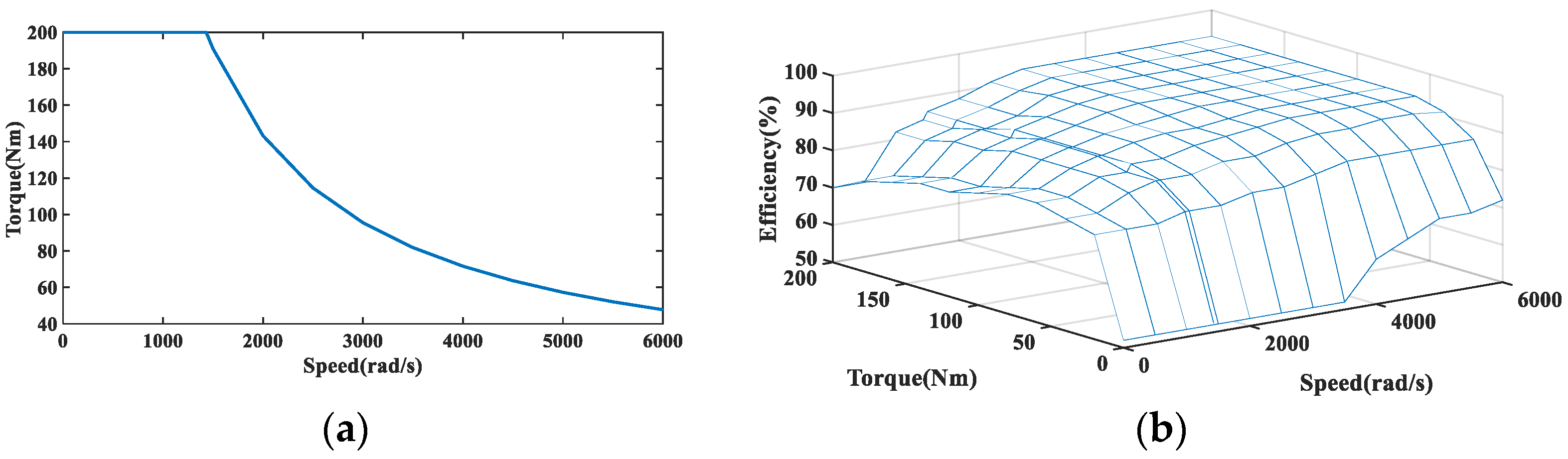
The powertrain assembly of a P2 configuration hybrid electric vehicle is widely used in the industry due to its simple design and better fuel economy [43]. In this study, an HEV with a P2 hybrid powertrain is used, and its electric motor is between the clutch and transmission. The powertrain topology is shown in Figure 10. The simulation model is a longitudinal dynamics model of the HEV on the basis of the rule-based strategy and its required driving force is as follows:

$$F_t=mgfcos\alpha +{\displaystyle \frac{1}{2}}{C}_d\rho A{v}^2+mgsin\alpha +\delta m{\displaystyle \frac{dv}{dt}}$$

(2)

where $F_t$ is the driving force, $m$ is the total vehicle mass, $\alpha$ is the road slope angle, $C_d$ is the air resistance coefficient, $\rho$ is the air density, $A$ is the windward area, $v$ is the vehicle velocity, and $\delta$ is the rotating mass conversion factor.

The vehicle dynamics model on the basis of longitudinal dynamics principles can precisely predict the required energy and enhance the simulation authenticity [44]. The shift law of the model includes two control parameters: pedal opening and vehicle velocity. The transmission is a multi-speed gearbox with six-speed configuration. Moreover,

Table 5. Main parameters of model.

Items	Parameters	Value
Vehicle	Mass	1620 kg
	Windward area	2.46 m2
Engine	Displacement	1.5 L
	Maximum torque	175 Nm
Motor	Maximum power	30 kW
	Maximum torque	200 Nm
Battery	Capacity	5.3 Ah
Transmission system	Transmission ratio	0.772–4.212
	Main reduction ratio	3.35

lists the principal arguments of the simulation model.

3.1.2. Motor Model

The motor plays the role of providing driving energy and charging battery in the hybrid power system and its main characteristics can be reflected by the external characteristic curve and efficiency map, as shown in Figure 11. Therefore, in this study, the electromagnetic thermal effect of the motor is ignored, and the static numerical method is used to establish the motor model.

$$P_{mech}=w \ast T$$

(3)

$$I={\displaystyle \frac{P_m+P_{loss}}{V_{bat}}}$$

(4)

$P_{mech}$ is the motor mechanical power, $w$ is motor speed, $T$ is motor torque, $I$ is the current of the battery, $P_{loss}$ is power loss, and $V_{bat}$ is battery voltage.

3.1.3. Power Battery Model

Because the internal resistance equivalent circuit model is simple to calculate and has good real-time performance, it is used in this study. The SOC value indicates the ratio of the current remaining charge in the battery to the fully charged battery in the current state, which is an important basis for monitoring the performance of the battery. Currently, the ampere–time integration method is the most common method for SOC estimation, and the ampere–time integration method is used to evaluate the SOC value in this study. The equivalent circuit model parameters and SOC value calculation formula are as follows:

$$U_{bat}=U_{oc}-I_{bat}{R}_{int}$$

(5)

$$SOC\left(t\right)=SOC\left(t_0\right)+{\int }_{t_0}^t{\displaystyle \frac{I_{bat}}{Q}}dt$$

(6)

where $U_{bat}$ is the terminal voltage of the power battery; $U_{oc}$ is the open-circuit voltage of the power battery, which can be obtained by checking the table according to the SOC value; $I_{bat}$ is the charging and discharging current of the battery; $R_{int}$ is the internal resistance of the power battery, which can be obtained by checking the table from the temperature and SOC; and $P_{bat}$ is the output power of the battery. $SOC\left(t\right)$ is the state of charge at time $t$, $SOC\left(t_0\right)$ denotes the initial charging state, and $Q$ is the capacity of the battery.

3.2. Model Simulation Results and Discussion

The full components of the HEV are modeled as sub-models. The approach to powertrain simulation is to analyze the state of each component by the input driving condition information. Moreover, according to longitudinal dynamics simulation, the required torque for each powertrain component is confirmed, as well as the analysis of fuel and energy consumption. To ensure that the model fulfills the driving requirements of user driving cycles, the HEV model is first simulated under the user driving cycle constructed in the previous section. In addition, the vehicle must also meet the driving demand of the standard driving cycle in real life. For this reason, this paper simulates the model under the standard working conditions of WLTC, NEDC, and FPT-75. The main results are as follows:

Figure 12 shows the velocity following and real-time deviation of velocity under the above four driving cycles, respectively. It demonstrates that the simulated velocity is basically consistent with the target velocity under the corresponding cycle, respectively. The deviations between the simulated velocity and target vehicle velocity under the four driving cycles are small, and the deviations are larger only in a few moments. And the average absolute deviations of velocity in user condition, WLTC condition, NEDC condition, and FTP-75 condition are 0.2661 m/s, 0.3051 m/s, 0.2816 m/s, and 0.4187 m/s, respectively. Start–stop, acceleration, and deceleration are more common in the FTP-75 condition and the deviations of the simulated vehicle velocity from the target velocity are larger near the target speed of zero, which leads to larger average absolute deviations. But it is a normal phenomenon, and the final deviations are still within a reasonable range. Therefore, the velocity of the model is good under the four driving cycles.

As shown in Figure 13, the trends of motor torque and battery current under the four driving cycles are basically the same, which correspond with the reality that motor torque and battery current are positively correlated as a whole, and the simulation of the model works well.

The SOC value is an important basis for monitoring the performance of the battery. Figure 14 shows the SOC parameter curve of the power battery, and the initial value of the battery SOC is 60%. It demonstrates that after operating on user driving condition, WLTC, NEDC, and FTP-75, respectively, the corresponding final SOC values are 43.38%, 32.31%, 43.11%, and 38.11%, which indicates the battery’s charging state is stable and the model simulation effect is better. In the vicinity of 1520–1730 s, the WLTC driving cycle has higher velocity and higher acceleration and duration. During this time, the motor is providing positive torque, and the battery is in a discharged state. Meanwhile, there is less deceleration process, low braking energy recovery, and the battery is continuously discharged. Therefore, the final SOC value of the WLTC driving cycle is the lowest among the four driving cycles.

Due to the existence of batteries in hybrid vehicles, when carrying out economic research on hybrid vehicles to calculate “fuel consumption”, engine FC needs to be considered. In addition, the electrical energy consumed by the battery should be converted into EFC to be accumulated in the total FC. To unify the evaluation indexes, the total fuel consumption is usually converted into 100 km EFC and used to evaluate the economy of hybrid vehicles. As shown in Figure 15, the 100 km EFC of the model under user condition, WLTC, NEDC, and FTP-75 are 5.7245 L, 5.8325 L, 5.5298 L, and 6.0717 L, respectively.

In summary, the model can meet the driving requirements of various working conditions with good dynamics, and the 100 km EFC is within a reasonable range under the corresponding driving cycle with good economy, so it can be used as the basis for the optimization of the hybrid vehicle’s economy.

4. Optimization of Hybrid Powertrain Parameters

4.1. Establishment of Optimization Target

In addition to the FC of the engine, the energy loss of the power battery should also be considered for the economy of the HEV. In this study, the energy loss of the power battery in a driving cycle is equivalent to the corresponding FC, and it is accumulated into the FC of the engine, so as to obtain the total equivalent fuel consumption. Then, in order to unify the evaluation criteria, it is converted into 100 km EFC, and it is regarded as the optimization objective. On the premise of ensuring that the vehicle can meet the driving requirements of the constructed working conditions, the appropriate optimization algorithm is found to improve the control and component parameters and achieve the goal of improving the overall economy of the vehicle. The specific process is as follows: every 100 kilometers the vehicle travels, the amount of gasoline consumed by the engine is $F_c$ L, and the energy consumed by the battery is $E_c$ kwh. Then in accordance with the equivalent principle of “33.7 kwh of electricity is equivalent to the energy content of a gallon of fuel” set by the United States Environmental Protection Agency (EPA). The equivalent amount of gasoline consumed by the battery is $E_c$/33.7 gallons, that is, the equivalent amount of gasoline consumed is equal to $E_c$/33.7 × 3.7854 L. The total 100 km EFC is as follows:

$$f=F_c+{\displaystyle \frac{3.7854}{33.7}} \ast E_c$$

(7)

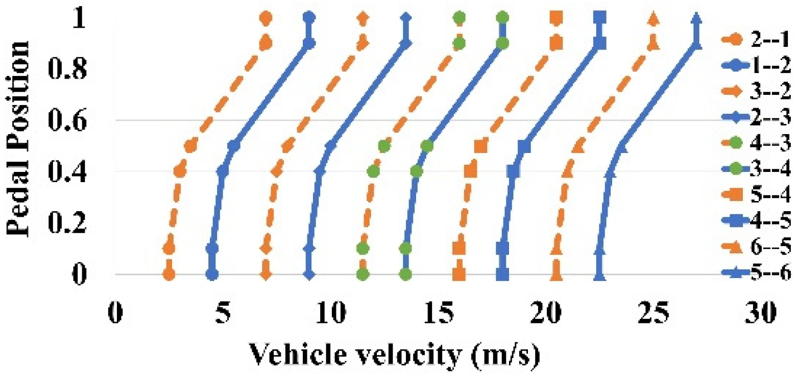
4.2. Selection of Optimization Variables

The choice of shift points has a significant impact on the FC and energy consumption of hybrid vehicles. In order to realize the overall change in shift points and simplify the workload as much as possible, this paper firstly parameterizes the shift schedule, and uses $c_1$ and $c_2$ as shift factors to realize the overall change in the shift schedule. The specific process is as follows:

$$pedal=\left[\begin{array}{c}{p}_{11}\\ p_{21}\\ p_{31}\\ p_{41}\end{array}\right]=\left[\begin{array}{c}0.1\\ 0.4\\ 0.5\\ 0.9\end{array}\right];a=\left[\begin{array}{c}{a}_{11}\\ a_{21}\\ a_{31}\\ a_{41}\end{array}\right]=\left[\begin{array}{c}3.5\\ 4.0\\ 4.5\\ 8.0\end{array}\right];$$

(8)

$$b=\left[\begin{array}{ccccc}{b}_{11}& b_{12}& b_{13}& b_{14}& b_{15}\\ b_{21}& b_{22}& b_{23}& b_{24}& b_{25}\\ b_{31}& b_{32}& b_{33}& b_{34}& b_{35}\\ b_{41}& b_{42}& b_{43}& b_{44}& b_{45}\end{array}\right]$$

(9)

where $b_{ij}=a_{i1}+c_1 * (j-1)+c_2 * (j-1) * p_{i1},(1\le i\le \mathrm{4,1}\le j\le 5)$.

$${shift}_{ij}=b_{ij}+∆/2; {shift\_1}_{ij}=b_{ij}-∆/2.$$

(10)

where $∆=2$; $∆$ is the difference between the corresponding upshift velocity and downshift velocity, and the units of $∆$, $b_{ij}$, ${shift}_{ij}$, and ${shift\_1}_{ij}$ are all $\mathrm{m}/\mathrm{s}$.

The shift threshold for a pedal opening of 0 to 0.1 is the same as when the pedal opening is 0.1. Meanwhile, the shift threshold for a pedal opening of 0.9 to 1 is the same as when the pedal opening is 0.9. At the initial time, the shift factor $c_1$ is equal to 4.5 and $c_2$ is equal to 0. At this point, the shift schedule is shown in Figure 16.

In addition to the shift points having a large impact on the economy of the hybrid vehicle, the main reduction ratio also affects the economy of the whole vehicle in the same way. Therefore, the total optimization variables selected in this paper are as follows: $X=\left[\begin{array}{ccc}{X}_1& X_2& X_3\end{array}\right]=\left[\begin{array}{ccc}{i}_0& c_1& c_2\end{array}\right]$. Where $i_0$ is the main reduction ratio, and $c_1$ and $c_2$ are the constants that realize the overall change in the shift schedule.

Considering factors, such as practical significance and cost, the specific constraints identified in this paper are as follows:

$$3\le i_0\le 5, 3.95\le c_1\le 5,-0.5\le c_2\le 0.5.$$

(11)

4.3. Optimization Method and Results

4.3.1. Fundamentals of WOA

In 2016, Mirjalili and Lewis raised WOA due to being motivated by the humpback whale’s amazing hunting behavior in the ocean [45]. WOA is a relatively new optimization algorithm with a simple but powerful search mechanism, fast tracking behavior, clear structure, few adjustment parameters, and is simple to implement [46], so it has been applied in various fields. WOA mainly includes three aspects: encirclement, bubble net attack, and random search for prey. The specific process is shown in Figure 17.

• Encircle prey stage: After recognizing the prey, individual whales will transmit the prey’s location information to the group, and other whales will approach the prey location to encircle them. This behavior can be expressed by the following equation:

$$\left\{\begin{array}{c}\overrightarrow{D}=\left|\overrightarrow{C}·{\overrightarrow{X}}_{Best}(t)-\overrightarrow{X}(t)\right|\\ \overrightarrow{X}(t+1)={\overrightarrow{X}}_{Best}(t)-\overrightarrow{A}·\overrightarrow{D}\\ \overrightarrow{A}=2\overrightarrow{a}·\overrightarrow{r}-\overrightarrow{a}\\ \overrightarrow{C}=2·\overrightarrow{r}\end{array}\right.$$

(12)

where $t$ is the number of current iteration generations, $\overrightarrow{A}$ and $\overrightarrow{C}$ are vectors of coefficients, ${\overrightarrow{X}}_{Best}(t)$ is the position vector of the current optimal solution, $\overrightarrow{X}(t)$ is the position vector of the current solution, and $\overrightarrow{X}(t+1)$ denotes the position vector of the $t+1$ generation solution. $\overrightarrow{a}$ is the vector that decreases linearly from 2 to 0 during the iteration, and $\overrightarrow{r}$ is a random vector between 0 and 1.

2.

Bubble net attack: The whale first estimates the distance to its prey and then slowly approaches the prey’s position. The process of capturing the prey by forming a spiral of bubbles around the prey can be represented as follows:

$$\overrightarrow{X}\left(t+1\right)=\left|{\overrightarrow{X}}_{Best}(t)-\overrightarrow{X}(t)\right|·{\mathrm{e}\mathrm{x}\mathrm{p}}^{bl}·\mathrm{c}\mathrm{o}\mathrm{s}(2\pi l)+{\overrightarrow{X}}_{Best}(t)$$

(13)

where $b$ is the spiral trajectory related parameter, and $l$ is a randomly generated decimal between −1 and 1.

When whales are feeding on prey, the encirclement and bubble net attack can be carried out simultaneously, so random numbers are used to realize the transformation of the hunting strategy. The mathematical model is represented as follows:

$$\overrightarrow{X}\left(t+1\right)=\left\{\begin{array}{c}{\overrightarrow{X}}_{Best}(t)-\overrightarrow{A}·\left|\overrightarrow{C}·{\overrightarrow{X}}_{Best}(t)-\overrightarrow{X}(t)\right|, p<0.5\\ \left|{\overrightarrow{X}}_{Best}(t)-\overrightarrow{X}(t)\right|·{\mathrm{e}\mathrm{x}\mathrm{p}}^{bl}·cos(2\pi l)+{\overrightarrow{X}}_{Best}(t), p\ge 0.5\end{array}\right.$$

(14)

where $p$ is a random number uniformly distributed between 0 and 1 that is used to determine which method an individual whale uses to update its position.

3.

Random search: When judging the parameters $|\overrightarrow{A}|\ge 1$, the whale will choose its search agent to iteratively optimize toward a random individual position, perform a random search away from the present position, and search for the globally optimal solution. Its mathematical model is as follows:

$$\left\{\begin{array}{c}{\overrightarrow{D}}_{rand}=\left|\overrightarrow{C}·{\overrightarrow{X}}_{rand}(t)-\overrightarrow{X}(t)\right|\\ \overrightarrow{X}(t+1)={\overrightarrow{X}}_{rand}(t)-\overrightarrow{A}·{\overrightarrow{D}}_{rand}\end{array}\right.$$

(15)

where ${\overrightarrow{X}}_{rand}(t)$ denotes the random position vector selected from the current population, and ${\overrightarrow{D}}_{rand}$ denotes the distance vector between this random whale and the rest of the whales.

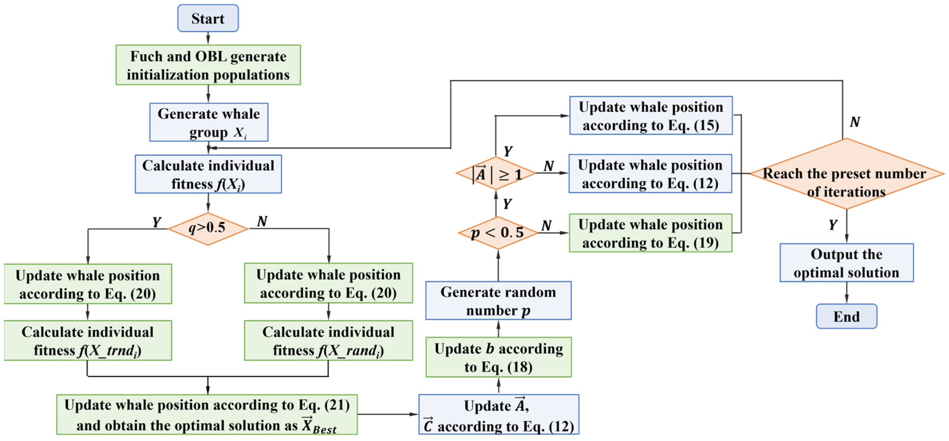
4.3.2. Fundamentals of MIWOA

Although WOA has many advantages, it still has problems such as dependence on initial population [47], insufficient search diversity, and can easily fall into local optimality [48]. To overcome these problems and enhance the algorithm’s optimization ability, this paper proposes MIWOA. The improvements are specified as follows, and the flowchart of MIWOA is shown in Figure 18.

• Fuch chaotic mapping is combined with OBL to generate more diverse initial populations.

The diversity of the initial population and the uniformity of variables’ spatial distribution will significantly affect the solving capability, as well as convergence speed, of the WOA. The initial population of traditional WOA is randomly created, so its distribution can easily become too concentrated, lack diversity, and have pseudo-randomness. However, the initial population generated by the Fuch chaotic map has good ergodicity, uniformity, and convergence [49]. The OBL strategy proposed by Tizhoosh et al. [50] computes and simultaneously evaluates the corresponding inverse solution for any feasible solution, and then selects the superior solution as the subsequent individual with a higher probability of reaching the global optimum. Therefore, this paper proposes to combine Fuch with OBL to enhance the initial population’s diversity and the convergence ability of solution exploration. The specific process is as follows:

Firstly, a population $X_i$ is generated according to Equation (16) and the corresponding inverse solution ${\overline{X}}_i$ is generated according to Equation (17). Then, $X_i$ and ${\overline{X}}_i$ are merged into one population and the fitness values of each set of solutions of the merged population are calculated separately. The merged population is sorted according to the fitness from smallest to largest, and the result is denoted as $X_{sort}$. Finally, the solutions with the same dimension as $X_i$ are taken sequentially from $X_{sort}$ as the initial population.

$$X_i=\cos ({\displaystyle \frac{1}{{X_{i-1}}^2}})$$

(16)

$${\overline{X}}_i=lb+ub-X_i$$

(17)

where $X_{i-1}$ is the chaotic variable of the Fuch mapping; $lb$ and $ub$ represent the minimum and maximum boundaries, respectively; and ${\overline{X}}_i$ refers to the inverse point corresponding to $X_i$

2.

Variable spiral parameter.

The spiral control parameter $b$ in Equation (13) is usually a constant. But if it is a fixed value, the whale will search for prey based on a fixed spiral every time. This will lead to a single way of moving the spiral, which is prone to fall into local optimization. To address this problem, the spiral control parameter is set as a variable that varies with the number of iterations, and Equation (19) is used instead of Equation (13) in the process of algorithm iteration. Thus, the spiral shape during whale search is dynamically adjusted to enrich the form of the whale’s position update and increase the whale’s exploration ability, which in turn improves the global search capability of the algorithm. The new formula for calculating the spiral parameter $b^{\prime }$ and Equation (19) are as follows:

$$b^{\prime }=1.5-\cos ({\displaystyle \frac{\pi }{2}} \mathrm{*} (1-{\displaystyle \frac{t}{T}}))$$

(18)

$$\overrightarrow{X}\left(t+1\right)=\left|{\overrightarrow{X}}_{Best}(t)-\overrightarrow{X}(t)\right|·{\mathrm{e}\mathrm{x}\mathrm{p}}^{b^{\prime }l}·\mathrm{c}\mathrm{o}\mathrm{s}\left(2\pi l\right)+{\overrightarrow{X}}_{Best}\left(t\right)$$

(19)

where $b^{’}$ is the variable spiral parameter.

3.

The adaptive weights are combined with t-distribution and random perturbation, respectively.

The solution value of the algorithm will always remain the same if the algorithm is at a local optimum during the iteration process. The t-distribution has good robustness and smoothness. The weight is adjusted according to the number of iterations, which is adaptive. The adaptive t-distribution perturbation combining adaptive weights and t-distribution perturbation show different exploration capabilities in the early and late iterations of the algorithm, which is conducive to improving the convergence speed of the algorithm’s convergence speed. Similarly, the adaptive random perturbation can also increase the optimization algorithm to jump out of the local optimal solution, thereby raising the likelihood of finding the global optimal and improving the algorithm’s robustness and adaptability. Therefore, this paper introduces adaptive weighted t-distribution perturbation and adaptive random perturbation into WOA. The calculation formula is as follows:

$$\left\{\begin{array}{c}{{X\_}_{trnd}}_i=X_i+\mathrm{g} \ast X_i \ast trnd\left(t\right), rand>0.5\\ {{X\_}_{rand}}_i=X_i+{\mathrm{g}}_1 \ast rand, rand>0.5\end{array}\right.$$

(20)

$$X_i=\left\{\begin{array}{c}{{X\_}_{trnd}}_i, f\left({{X\_}_{trnd}}_i\right)<f\left(X_i\right)\\ {{X\_}_{rand}}_i, f\left({{X\_}_{rand}}_i\right)<f\left(X_i\right)\end{array}\right.$$

(21)

where $rand$ is a random number between 0 and 1; ${{X\_}_{trnd}}_i$ is the solution of $X_i$ after adaptive weighted t-distribution perturbation; $\mathrm{g}$ is the adaptive weight corresponding to the t-distribution perturbation, $\mathrm{g}=0.4+0.1 \mathrm{*} \sin \left({\displaystyle \frac{T-t}{T}}\right)$; $trnd\left(t\right)$ is the t-distribution with the current number of iterations as degrees of freedom; ${{X\_}_{rand}}_i$ is the solution of $X_i$ after adaptive random perturbation strategy; ${\mathrm{g}}_1$ is the adaptive weight corresponding to the random perturbation strategy, ${\mathrm{g}}_1=-0.4+0.5 \mathrm{*} \cos ({\displaystyle \frac{T-t}{T}})$; and $f\left({{X\_}_{trnd}}_i\right)$, $f\left(X_i\right)$, $f\left({{X\_}_{rand}}_i\right)$ are the fitness values for ${{X\_}_{trnd}}_i$, $X_i$, and ${{X\_}_{rand}}_i$, respectively.

If the position of the solution generated after perturbation is superior to the original position, the original solution is replaced with it to make it a better solution. Conversely, the position of the solution remains unchanged. Then, the new solution is compared with the current optimal solution, and if the new solution is superior, then it is assigned to the optimal solution. Otherwise, the original optimal solution remains unchanged.

4.4. Optimization Results and Discussion

Under the user driving cycle synthesized in Section 2, the objective function is defined according to Section 4.1, the algorithm iteration times are set to 40, the main deceleration ratio and shift factors are selected as optimization variables, the GA method, WOA method and MIWOA codes are written, and the hybrid vehicle model is invoked to complete the HEV economic optimization. Figure 19 shows the change of 100 km EFC in the iterative optimization process. As the times of optimization iterations grow, the 100 km EFC gradually decreases and converges. Obviously, compared with the GA and WOA methods, the MIWOA method shows better a optimization effect and obtains better economic optimization results. This is mainly because the combination of Fuch and OBL enhances the initial population’s diversity, which solves the problem of pseudo-randomness in the initial population of the original algorithm created by the randomized method. In addition, OBL can make the algorithm start from the region of the optimal solution, which increases the possibility of obtaining the global optimal solution. The proposed variable spiral parameter enriches the whale search and improves the algorithm’s ability of global exploration. The adaptive t-distribution perturbation and adaptive random perturbation optimize the algorithm iteration process and increase the likelihood of jumping out of the local optimum.

In this paper, the optimization results of the MIWOA method are finally selected as the optimal result. The optimized main reduction ratio, as well as shift factors, both meet the constraint conditions, and the optimization results are reliable. After optimization, $i_0$, $c_1$, and $c_2$ are 3, 4.2781, and 0.3184, respectively. At this point, the objective function value is minimized, and the economy is optimal. To further verify the effectiveness of the MIWOA-based optimization powertrain parameters under user driving cycles and standard driving cycles, the optimized variables are input into the HEV model, and the model is simulated again under the above four driving cycles. The specific results are as described later.

Figure 20 shows the velocity curves and their instantaneous deviations of the optimized model for the user driving cycle, WLTC, NEDC, and FTP-75, successively. They demonstrate that the deviations of the simulated actual velocity from the target velocity under the four driving cycles are small, and the deviations are only slightly larger in a few moments. Similarly, the overall fluctuation is small, and the velocity following is good, so that the simulated actual velocity is basically the same as the target velocity. Therefore, the optimized model can meet the velocity and acceleration requirements of the driving cycles. The dynamic performance of the HEV model is good, which provides a significant reference for accurately evaluating the vehicle economy.

Shift decisions are aimed at ensuring power and driving performance while minimizing EFC, and reasonable shift strategies are crucial for improving overall economy, performance, and comfort [51]. The optimization of gearshift moments using global optimization algorithms is usually completed under some standard driving cycles, while the user’s actual driving situation differs greatly from the standard driving cycle. Correspondingly, the generated user driving cycle in this research are closer to the actual driving conditions of the users of the vehicles, which provides an important guarantee for the optimization of gearshift laws. Based on the user driving cycle, intelligent algorithms are used to find economic shift strategies, which provide an important program for improving the economy of the powertrain. The shift curves of first gear up to second gear and second gear down to first gear is taken as the benchmark, and the shift factors are used to adjust the thresholds of the rest of the shift lines to correct the shift curves. After optimization, except for the benchmark lines, which keep the original setting, the shift thresholds of the other gears are lower than those of the original shift lines, as shown in Figure 21. In addition, combining Figure 20 and Figure 22, it can be seen that when the shift schedule is changed, the EFC of the vehicle is reduced, but the dynamics of the vehicle can still satisfy the power demands of a wide range of operating conditions. Therefore, the optimized shift schedule can achieve the purpose of improving economy while maintaining dynamics and solves the problem of difficulty in selecting shift moments.

The 100 km EFC of the final model optimized based on user driving cycles is 5.4271 L, which is 0.2974 L lower than that of the pre-optimization, and the economy is improved by 5.20%, which is a better optimization effect. In addition, the optimized model was simulated for economy under the WLTC driving cycle, NEDC, and FTP-75, respectively. Figure 22 and

Table 6. Comparison of results before and after optimization.

Items	Before Optimization	After Optimization	Improvement
i0	3.35	3	-
c1	4.5	4.2781
c2	0	0.3184
User EFC(L/100 km)	5.7245	5.4271	5.20%
WLTC EFC (L/100 km)	5.8325	5.6220	3.61%
NEDC EFC (L/100 km)	5.5298	5.1435	6.99%
FTP-75 EFC (L/100 km)	6.0717	5.9305	2.33%

show the 100 km EFC for different driving cycles, respectively. The final 100 km EFC of WLTC is 5.6220 L, which is 0.2105 L lower than that of the pre-optimization, and the economy is improved by 3.61%; the 100 km EFC of NEDC is 5.1435 L, which is 0.3863 L lower than that of the pre-optimization, and the economy is improved by 6.99%. Moreover, the 100 km EFC of FTP-75 is 5.9305 L, which is 0.1412 L lower than that of the pre-optimization, and the economy is improved by 2.33%. Under different driving cycles, the economy is improved to a certain extent, which proves the effectiveness of MIWOA in optimizing the parameters of the hybrid powertrain to improve vehicle economy. Under different cycles, the economy improvement varies, so it is essential to generate user driving cycles for user groups.

The results of the SOC value provide an important reference for evaluating the operational performance of the battery under various driving cycles. Figure 23 shows the comparison of the SOC parameter curves of the power battery before and after optimization under four driving cycles. The initial value of the battery SOC is 60%. After one user driving cycle, WLTC, NEDC, and FTP-75, respectively, the final SOC values are 38.96%, 27.68%, 40.67%, and 39.27%. This suggests that the status of the power battery is more stable, and the model simulation effect is better. Before and after optimization, the curves of SOC show the same trend, and the optimized SOC value will be lower than the pre-optimization one in most moments. The percentage of battery participation in the cycle is increased, which improves the economy of the whole vehicle. The final SOC values of user driving condition, WLTC, and NEDC are all lower than those before optimization, while the final SOC values change the least under FTP-75. The reason for this outcome is that the FTP-75 condition has a more significant deceleration process and higher braking energy recovery rate.

5. Conclusions

This paper raises a method flow of HEV economy optimization based on user driving cycles. The study uses a stepwise regression method to complete the selection of characteristic parameters oriented to average instantaneous fuel consumption characteristics, which addresses the problem of randomness in the choice of feature parameters. The SAGAFCM method was employed for constructing the user driving cycle that is more representative and in line with the actual driving characteristics. Then, the constructed condition is used as the target driving cycle for hybrid powertrain economy optimization, which provides a more accurate basis for the performance evaluation of the vehicle. Simultaneously, it provides an important reference for enterprises to optimize vehicle performance or develop new generation models, which is of great significance to improve user satisfaction and experience.

Under the user driving cycle, a hybrid vehicle optimization model based on MIWOA is constructed, and this study proposes the MIWOA method to optimize the shift schedule and the main reduction ratio of the powertrain of HEV to obtain the economic parameters of the hybrid vehicle that are more in line with the user’s actual driving conditions. The combination of Fuch and OBL enhances the initial population’s diversity and the algorithm’s convergence capacity, which solves the problem of pseudo-randomness in the initial population created by the random method of the original algorithm. The proposed variable spiral parameter enriches search mode and improves the global exploration ability. The adaptive weights are combined with t-distribution perturbation and random perturbation, respectively, to improve the likelihood of jumping out of the local optimum.

After the optimization, the 100 km EFC of the whole vehicle is lowered by 5.20% under the user driving cycle, which effectively brings into play the energy-saving potential of the powertrain and enhances the vehicle’s economic performance. In addition, considering that the optimized vehicle model should also meet the driving requirements of standard driving cycles, this paper carries out economic simulation of the optimized model based on the standard driving cycles of WLTC, NEDC, and FTP75, respectively, and the simulation results show that their economy is improved to a certain extent. The findings provide a driving cycle that is closer to the actual driving conditions of users for manufacturers when developing vehicles. Meanwhile, this study demonstrates the effectiveness of the proposed MIWOA method in improving vehicle economy, obtains the economy parameters that are more suitable for the user driving cycle, and contributes a new idea and methodology for the optimization of the hybrid powertrain economy.

The focus of future work is to improve the control strategy by using machine learning and other methods based on this study and improve the adaptability of hybrid electric vehicles to actual roads.

References

1. Guo, L.; Hu, P.; Wei, H. Development of supercapacitor hybrid electric vehicle. J. Energy Storage 2023, 65, 107269. [Google Scholar] [CrossRef]
2. Huang, R.; He, H.; Su, Q.; Härtl, M.; Jaensch, M. Enabling cross-type full-knowledge transferable energy management for hybrid electric vehicles via deep transfer reinforcement learning. Energy 2024, 305, 132394. [Google Scholar] [CrossRef]
3. Shuai, Z.; Li, C.; Gai, J.; Han, Z.; Zeng, G.; Zhou, G. Coordinated motion and powertrain control of a series-parallel hybrid 8 × 8 vehicle with electric wheels. Mech. Syst. Signal Process. 2018, 120, 560–583. [Google Scholar] [CrossRef]
4. Xue, J.; Jiao, X.; Yu, D.; Zhang, Y. Predictive hierarchical eco-driving control involving speed planning and energy management for connected plug-in hybrid electric vehicles. Energy 2023, 283, 129058. [Google Scholar] [CrossRef]
5. Ruan, S.; Ma, Y.; Yang, N.; Yan, Q.; Xiang, C. Multiobjective optimization of longitudinal dynamics and energy management for HEVs based on nash bargaining game. Energy 2023, 262, 125422. [Google Scholar] [CrossRef]
6. Hu, X.; Zhang, X.; Tang, X.; Lin, X. Model predictive control of hybrid electric vehicles for fuel economy, emission reductions, and inter-vehicle safety in car-following scenarios. Energy 2020, 196, 117101. [Google Scholar] [CrossRef]
7. Berzi, L.; Delogu, M.; Pierini, M. Development of driving cycles for electric vehicles in the context of the city of Florence. Transp. Res. Part D Transp. Environ. 2016, 47, 299–322. [Google Scholar] [CrossRef]
8. Pacheco, F.; Cerrada, M.; Huertas, J.I. Threshold-guided multi-objective Generative Adversarial Networks for constructing artificial yet representative driving cycles. Eng. Appl. Artif. Intell. 2024, 129, 107665. [Google Scholar] [CrossRef]
9. Brady, J.; O’mahony, M. Development of a driving cycle to evaluate the energy economy of electric vehicles in urban areas. Appl. Energy 2016, 177, 165–178. [Google Scholar] [CrossRef]
10. Zhang, J.; Wang, Z.; Liu, P.; Zhang, Z.; Li, X.; Qu, C. Driving cycles construction for electric vehicles considering road environment: A case study in Beijing. Appl. Energy 2019, 253, 113514. [Google Scholar] [CrossRef]
11. Lei, N.; Zhang, H.; Li, R.; Yu, J.; Wang, H.; Wang, Z. Physics-informed data-driven modeling approach for commuting-oriented hybrid powertrain optimization. Energy Convers. Manag. 2024, 299, 117814. [Google Scholar] [CrossRef]
12. Wang, Y.; Li, K.; Zeng, X.; Gao, B.; Hong, J. Energy consumption characteristics based driving conditions construction and prediction for hybrid electric buses energy management. Energy 2022, 245, 123189. [Google Scholar] [CrossRef]
13. Zhuang, W.; Eben, S.L.; Zhang, X.; Kum, D.; Song, Z.; Yin, G.; Ju, F. A survey of powertrain configuration studies on hybrid electric vehicles. Appl. Energy 2020, 262, 114553. [Google Scholar] [CrossRef]
14. Qiu, H.; Cui, S.; Wang, S.; Wang, Y.; Feng, M. A Clustering-Based Optimization Method for the Driving Cycle Construction: A Case Study in Fuzhou and Putian, China. IEEE Trans. Intell. Transp. Syst. 2022, 23, 18681–18694. [Google Scholar] [CrossRef]
15. Peng, J.; Zhang, H.; Ma, C.; He, H. Powertrain Parameters’ Optimization for a Series–Parallel Plug-In Hybrid Electric Bus by Using a Combinatorial Optimization Algorithm. IEEE J. Emerg. Sel. Top. Power Electron. 2023, 11, 32–43. [Google Scholar] [CrossRef]
16. Lei, N.; Zhang, H.; Wang, H.; Wang, Z. An Improved Co-Optimization of Component Sizing and Energy Management for Hybrid Powertrains Interacting With High-fidelity Model. IEEE Trans. Veh. Technol. 2023, 72, 15585–15596. [Google Scholar] [CrossRef]
17. Cui, Y.; Xu, H.; Zou, F.; Chen, Z.; Gong, K. Optimization based method to develop representative driving cycle for real-world fuel consumption estimation. Energy 2021, 235, 121434. [Google Scholar] [CrossRef]
18. Tao, S.; Ding, K.; Li, Z.; Zhang, H. Development of a representative driving cycle for evaluating exhaust emission and fuel consumption for Chinese switcher locomotives. Appl. Energy 2022, 322, 119499. [Google Scholar] [CrossRef]
19. Hull, C.; Collett, K.A.; McCulloch, M.D. Developing a representative driving cycle for paratransit that reflects measured data transients: Case study in Stellenbosch, South Africa. Transp. Res. Part A Policy Pr. 2024, 181, 103987. [Google Scholar] [CrossRef]
20. Ma, R.; He, X.; Zheng, Y.; Zhou, B.; Lu, S.; Wu, Y. Real-world driving cycles and energy consumption informed by large-sized vehicle trajectory data. J. Clean. Prod. 2019, 223, 564–574. [Google Scholar] [CrossRef]
21. Zhang, M.; Shi, S.; Lin, N.; Yue, B. High-Efficiency Driving Cycle Generation Using a Markov Chain Evolution Algorithm. IEEE Trans. Veh. Technol. 2019, 68, 1288–1301. [Google Scholar] [CrossRef]
22. Nyberg, P.; Frisk, E.; Nielsen, L. Using Real-World Driving Databases to Generate Driving Cycles with Equivalence Properties. IEEE Trans. Veh. Technol. 2016, 65, 4095–4105. [Google Scholar] [CrossRef]
23. Ding, X.; Zhang, H.; Zhang, W.; Xuan, Y. Non-uniform state-based Markov chain model to improve the accuracy of transient contaminant transport prediction. Build. Environ. 2023, 245, 110977. [Google Scholar] [CrossRef]
24. Zhao, X.; Zhao, X.; Yu, Q.; Ye, Y.; Yu, M. Development of a representative urban driving cycle construction methodology for electric vehicles: A case study in Xi’an. Transp. Res. D Transp. Environ. 2020, 81, 102279. [Google Scholar] [CrossRef]
25. Yang, Y.; Li, T.; Zhang, T.; Yu, Q. Time dimension analysis: Comparison of Nanjing local driving cycles in 2009 and 2017. Sustain. Cities Soc. 2020, 53, 101949. [Google Scholar] [CrossRef]
26. Huzayyin, O.A.; Salem, H.; Hassan, M.A. A representative urban driving cycle for passenger vehicles to estimate fuel consumption and emission rates under real-world driving conditions. Urban Clim. 2021, 36, 100810. [Google Scholar] [CrossRef]
27. Wang, Z.; Zhao, L.; Kong, Z.; Yu, J.; Yan, C. Development of accelerated reliability test cycle for electric drive system based on vehicle operating data. Eng. Fail. Anal. 2022, 141, 106696. [Google Scholar] [CrossRef]
28. Tang, X.; Zhang, J.; Pi, D.; Lin, X.; Grzesiak, L.M.; Hu, X. Battery Health-Aware and Deep Reinforcement Learning-Based Energy Management for Naturalistic Data-Driven Driving Scenarios. IEEE Trans. Transp. Electrif. 2022, 8, 948–964. [Google Scholar] [CrossRef]
29. Azad, S.; Alexander-Ramos, M.J. Robust Combined Design and Control Optimization of Hybrid-Electric Vehicles Using MDSDO. IEEE Trans. Veh. Technol. 2021, 70, 4139–4152. [Google Scholar] [CrossRef]
30. Wang, Z.; Jiao, X. Optimization of the powertrain and energy management control parameters of a hybrid hydraulic vehicle based on improved multi-objective particle swarm optimization. Eng. Optim. 2021, 53, 1835–1854. [Google Scholar] [CrossRef]
31. Eckert, J.J.; Silva, F.L.; da Silva, S.F.; Bueno, A.V.; de Oliveira, M.L.M.; Silva, L.C. Optimal design and power management control of hybrid biofuel–electric powertrain. Appl. Energy 2022, 325, 119903. [Google Scholar] [CrossRef]
32. Zhou, Q.; Zhang, W.; Cash, S.; Olatunbosun, O.; Xu, H.; Lu, G. Intelligent sizing of a series hybrid electric power-train system based on Chaos-enhanced accelerated particle swarm optimization. Appl. Energy 2017, 189, 588–601. [Google Scholar] [CrossRef]
33. Jeoung, D.; Min, K.; Sunwoo, M. Automatic Transmission Shift Strategy Based on Greedy Algorithm Using Predicted Velocity. Int. J. Automot. Technol. 2020, 21, 159–168. [Google Scholar] [CrossRef]
34. Zhang, H.; Yang, X.; Sun, X.; Liang, J. Optimal Design of Shift Point Strategy for DCT Based on Particle Swarm Optimization. Machines 2021, 9, 196. [Google Scholar] [CrossRef]
35. Eckert, J.J.; da Silva, S.F.; Santiciolli, F.M.; de Carvalho, Á.C.; Dedini, F.G. Multi-speed gearbox design and shifting control optimization to minimize fuel consumption, exhaust emissions and drivetrain mechanical losses. Mech. Mach. Theory 2022, 169, 104644. [Google Scholar] [CrossRef]
36. Zhang, Y.; Wu, H.; Mi, S.; Zhao, W.; He, Z.; Qian, Y.; Lu, X. Comparative study of hybrid architectures integrated with dual-fuel intelligent charge compression ignition engine: A commercial powertrain solution towards carbon neutrality. Energy Convers. Manag. 2023, 292, 117423. [Google Scholar] [CrossRef]
37. Jia, Q.; Zhang, C.; Zhang, H.; Zhang, Z.; Chen, H. Powertrain parameters and control strategy optimization of a novel master-slave electric-hydraulic hybrid vehicle. Energy Sources Part A Recover. Util. Environ. Eff. 2023, 45, 11752–11773. [Google Scholar] [CrossRef]
38. Shen, P.; Zhao, Z.; Li, J.; Zhan, X. Development of a typical driving cycle for an intra-city hybrid electric bus with a fixed route. Transp. Res. Part D Transp. Environ. 2018, 59, 346–360. [Google Scholar] [CrossRef]
39. Song, T.; Zhu, W.-X.; Su, S.-B.; Wang, W.-W. Distributed “End-Edge-Cloud” structural car-following control system for intelligent connected vehicle using sliding mode strategy. Commun. Nonlinear Sci. Numer. Simul. 2023, 126, 107468. [Google Scholar] [CrossRef]
40. Yang, D.; Liu, T.; Zhang, X.; Zeng, X.; Song, D. Construction of high-precision driving cycle based on Metropolis-Hastings sampling and genetic algorithm. Transp. Res. Part D Transp. Environ. 2023, 118, 103715. [Google Scholar] [CrossRef]
41. Zhang, X.; Zhou, J.; Chen, W. Data-driven fault diagnosis for PEMFC systems of hybrid tram based on deep learning. Int. J. Hydrogen Energy 2020, 45, 13483–13495. [Google Scholar] [CrossRef]
42. Li, J. Research on Driving Condition Prediction and Adaptive Control Strategy of Plug-In Hybrid Electric Vehicle. Master’s Thesis, Jilin University, Changchun, China, 2020. [Google Scholar]
43. Gao, H.; Zhang, X.; Zeng, X.; Yang, D.; Song, D.; Zhou, L. Predictive cruise control for hybrid electric vehicles based on hierarchical convex optimization. Energy Convers. Manag. 2024, 299, 117883. [Google Scholar] [CrossRef]
44. Alpaslan, E.; Karaoğlan, M.U.; Colpan, C.O. Investigation of drive cycle simulation performance for electric, hybrid, and fuel cell powertrains of a small-sized vehicle. Int. J. Hydrogen Energy 2023, 48, 39497–39513. [Google Scholar] [CrossRef]
45. Nadimi-Shahraki, M.H.; Zamani, H.; Varzaneh, Z.A.; Mirjalili, S. A Systematic Review of the Whale Optimization Algorithm: Theoretical Foundation, Improvements, and Hybridizations. Arch. Comput. Methods Eng. 2023, 30, 4113–4159. [Google Scholar] [CrossRef]
46. Pham, Q.-V.; Mirjalili, S.; Kumar, N.; Alazab, M.; Hwang, W.-J. Whale Optimization Algorithm with Applications to Resource Allocation in Wireless Networks. IEEE Trans. Veh. Technol. 2020, 69, 4285–4297. [Google Scholar] [CrossRef]
47. Che, Z.; Peng, C.; Yue, C. Optimizing LSTM with multi-strategy improved WOA for robust prediction of high-speed machine tests data. Chaos Solitons Fractals 2024, 178, 114394. [Google Scholar] [CrossRef]
48. Yu, W.; Zhou, P.; Miao, Z.; Zhao, H.; Mou, J.; Zhou, W. Energy performance prediction of pump as turbine (PAT) based on PIWOA-BP neural network. Renew. Energy 2024, 222, 119873. [Google Scholar] [CrossRef]
49. Zhao, W.; Liu, Y.; Zhou, X.; Li, S.; Zhao, C.; Dou, C.; Shu, H. An aeration requirements calculating method based on BOD5 soft measurement model using deep learning and improved coati optimization algorithm. J. Water Process. Eng. 2024, 64, 105693. [Google Scholar] [CrossRef]
50. Tizhoosh, H.R. Opposition-based learning: A new scheme for machine intelligence. In Proceedings of the International Conference on Computational Intelligence for Modelling, Control and Automation and International Conference on Intelligent Agents, Web Technologies and Internet Commerce (CIMCA-IAWTIC’06), Vienna, Austria, 28–30 November 2005; Volume 1, pp. 695–701. [Google Scholar] [CrossRef]
51. Wang, S.; Zhang, K.; Shi, D.; Li, M.; Yin, C. Research on economical shifting strategy for multi-gear and multi-mode parallel plug-in HEV based on DIRECT algorithm. Energy 2024, 286, 129574. [Google Scholar] [CrossRef]
Figure 1. Hybrid powertrain parameters optimization model based on user driving cycle.
Machines 13 00158 g001
Figure 2. Schematic diagram of Internet of Vehicles data acquisition.
Machines 13 00158 g002
Figure 3. Kinematic segments and motion states.
Machines 13 00158 g003
Figure 4. Contribution and cumulative contribution of each principal component.
Machines 13 00158 g004
Figure 5. Clustering bias for different N values.
Machines 13 00158 g005
Figure 6. Flowchart of SAGAFCM algorithm.
Machines 13 00158 g006
Figure 7. Scatter plot of clustering results of first three principal components.
Machines 13 00158 g007
Figure 8. Representative driving cycle of users’ real vehicles.
Machines 13 00158 g008
Figure 9. Characterization indicators and their relative errors.
Machines 13 00158 g009
Figure 10. Topology of powertrain system.
Machines 13 00158 g010
Figure 11. Motor (a) external characteristic curve and (b) efficiency map.
Machines 13 00158 g011
Figure 12. Velocity following and real-time deviation under (a) user driving cycle, (b) WLTC, (c) NEDC, (d) FTP-75.
Machines 13 00158 g012
Figure 13. Motor torque and battery current under (a) user driving cycle, (b) WLTC, (c) NEDC, (d) FTP-75.
Machines 13 00158 g013
Figure 14. Battery SOC under four driving cycles.
Machines 13 00158 g014
Figure 15. The 100 km equivalent fuel consumption under four driving cycles.
Machines 13 00158 g015
Figure 16. Gear shift schedule.
Machines 13 00158 g016
Figure 17. Flowchart of whale optimization algorithm.
Machines 13 00158 g017
Figure 18. Flowchart of multi-strategy improved whale optimization algorithm.
Machines 13 00158 g018
Figure 19. Optimization results of GA, WOA, and MIWOA.
Machines 13 00158 g019
Figure 20. Velocity following and instantaneous deviations under (a) user driving cycle, (b) WLTC, (c) NEDC, (d) FTP-75 after optimization.
Machines 13 00158 g020
Figure 21. Shift schedule before and after optimization.
Machines 13 00158 g021
Figure 22. Comparison of 100 km EFC before and after optimization under (a) user driving cycle, (b) WLTC, (c) NEDC, (d) FTP-75.
Machines 13 00158 g022
Figure 23. Comparison of SOC curves before and after optimization under (a) user driving cycle, (b) WLTC, (c) NEDC, (d) FTP-75.
Machines 13 00158 g023aMachines 13 00158 g023b