Abstract
Bearing-vibration signals, characterized by strong non-stationarity, typically consist of multiple components. The periodic pulses related to bearing faults are frequently obscured by surrounding noise, and early bearing-fault vibrations are feeble, which complicates the extraction of inherent fault characteristics. The aim of this research is to develop an effective method for extracting early-fault characteristic frequencies in rolling bearings. VMD, short for variational mode decomposition, is an innovative technique rooted in the classical Wiener filter for analyzing signals that include multiple components. However, applying VMD to process real non-stationary signals still poses several challenges. A key challenge is that the internal parameters of VMD require manual setting prior to use. Aiming to mitigate this limitation, this paper introduces an enhanced variational mode decomposition approach utilizing the Chaotic Harris Hawk Optimization (CHHO) method. Average energy entropy is used as the optimization criterion in the CHHO–VMD algorithm to ascertain both the ideal mode count and its corresponding penalty factor. The original signal is further broken down into intrinsic mode functions (IMFs), with each IMF corresponding to a different frequency interval. In addition, IMF components are selected based on kurtosis and cross-correlation criteria to reconstruct fault signals. Finally, envelope demodulation is performed to reveal the fault characteristic frequencies. Experimental findings demonstrate that, as opposed to alternative techniques, this approach achieves superior performance in extracting early-fault frequencies in rolling bearings, offering a novel solution for early-fault feature extraction.
1. Introduction
The most common elements of mechanical transmissions are rolling bearings [1]. Bearings, as the basic components of every machine, play a key role in the operation of machines, their maintenance, and their reliability because they are responsible for transferring loads [2]. As a fundamental component of large-scale industrial rotating machinery, rolling bearings are essential for improving the efficiency of mechanical systems. Their condition has a direct impact on the reliable performance of the equipment [3]. Thus, research into bearing faults holds significant practical value, particularly in ensuring production safety in relevant industries. Nevertheless, rolling bearings frequently operate under extreme conditions, such as high temperatures, high pressures, and complex surroundings, thereby increasing the risk of failure [4]. In addition, early-fault signals are weak and susceptible to environmental noise interference, and their vibration transmission paths are intricate, making fault feature extraction highly challenging. Therefore, accurately processing the raw vibration signals and effectively extracting fault characteristics are crucial for evaluating operational status, preventing accidents, and improving equipment performance [5].
Within the realm of rolling-bearing-fault signal analysis, several commonly used signal processing techniques exist. These include wavelet packet decomposition (WPT), empirical mode decomposition (EMD), ensemble empirical mode decomposition (EEMD), complete ensemble empirical mode decomposition (CEEMD), and local mode decomposition (LMD) [6]. However, WPT requires the prior selection of a wavelet basis function, which may influence the bearing fault signal’s decomposition results, as it lacks the ability for adaptive signal decomposition [7]. The EMD method has garnered significant attention since its introduction due to its adaptive capability for decomposing signals of interest [8]. EEMD is suggested to resolve the drawbacks of EMD, effectively mitigating the mode-mixing issue [9]. CEEMD addresses issues of remaining noise in the EEMD-rebuilt signal and variability in mode numbers resulting from different signal-plus-noise realizations [10]. Despite continuous advancements in the EMD method, both LMD and CEEMD perform adaptive decomposition based on signal characteristics but still suffer from limitations such as the absence of a rigorous mathematical model, the occurrence of mode mixing, and high sensitivity to noise [11].
To improve upon the limitations of the aforementioned nonlinear signal analysis techniques, a novel adaptive approach named variational mode decomposition was proposed [12]. The algorithm identifies the central frequency and bandwidth of every mode by repeatedly seeking the most suitable solution to a variational schema, thus enabling precise partitioning of the signal within the spectral range and the separation of its components. Each signal component is assumed to be a narrowband signal concentrated around its center frequency in VMD. Under this assumption, a series of narrowband Wiener filters are designed to tackle the issue of constrained optimization, facilitating the extraction of corresponding signal components. VMD is grounded in a rigorous mathematical foundation and exhibits strong noise robustness. Therefore, in recent years, VMD method has been widely used in mechanical equipment vibration signal processing [13,14]. However, it necessitates the prior selection of hyperparameters, such as the mode count and penalty factor . Incorrect selection of these parameters may lead to excessive decomposition or insufficient decomposition. Consequently, in recent years, numerous scholars, both domestically and internationally, have proposed optimization algorithms to adaptively explore optimal values of and . In 2020, Ding et al. [15] introduced a method integrating genetic mutation, particle swarm optimization, and variational mode decomposition (GM–PSO–VMD) to obtain fault characteristics from the corresponding signals. This algorithm’s performance was validated by comparing its outcomes with those of fixed-parameter VMD (FP–VMD) and the EMD method. With the aim of improving the extraction of bearing-fault features, Li et al. [16] introduced a method integrating genetic algorithm with variational mode decomposition (GA–VMD). To address shortcomings of conventional characteristic extraction techniques in noise suppression and periodic weak fault detection, Mingzhu Lv [17] and colleagues proposed a novel approach that integrates the envelope harmonic-to-noise ratio (EHNR) with an adaptive variational mode decomposition (AVMD). This AVMD method utilizes the grey wolf optimization (GWO) approach [18]. Furthermore, the study introduces a novel metric, termed effective weighted sparseness kurtosis, which enhances the identification of IMF modes. To fully leverage the superiority of VMD for noise suppression and the effectiveness of maximum correlation kurtosis deconvolution for stressing successive pulses obscured by noise, Liu et al. [19] put forward a technology that integrates the sparrow search algorithm, VMD and MCKD, referred to as SSA–VMD–MCKD, to extract weak faults of rolling bearings. Wang et al. [20] employed the beetle antennae search (BAS) algorithm to fine-tune parameters associated with VMD. The IMF exhibiting the highest kurtosis was chosen as the most responsive component. The corresponding envelope spectrum successfully highlighted key fault impulse characteristics. Jin et al. [21] integrated chaotic mapping, nonlinear convergence coefficient, and inertia weight the within whale optimization algorithm (WOA), resulting in an enhanced version known as the improved whale optimization algorithm. VMD parameters are optimized using this technique, and this enhanced VMD, in conjunction with sample entropy, is subsequently employed for signal denoising and reconstruction. Heidari et al. [22] proposed a new intelligent optimization algorithm called Harris Hawks Optimization (HHO) in 2019. The effectiveness of the proposed HHO technique was assessed by comparing it to other bio-inspired methods across 29 test problems and a range of engineering tasks.
While traditional intelligent optimization algorithms have demonstrated some effectiveness in optimizing VMD parameters, they continue to encounter issues such as high computational cost, redundancy, low efficiency, difficulties in full-range search, and the tendency to get stuck in local extrema. In the study, the HHO technique was improved, and the enhanced algorithm is called the Chaotic Harris Hawk Optimization algorithm [23,24,25]. The CHHO algorithm is leveraged for optimizing and , two vital parameters of VMD. The key contributions of the CHHO–VMD algorithm are as follows:
- (1)
- For the purpose of enhancing the variety within the population and improving the equilibrium between exploration and exploitation in the HHO technique, chaotic mapping, a nonlinear reduction factor, and Gaussian mutation were incorporated.
- (2)
- The CHHO algorithm is deployed to dynamically optimize and determine the parameter combination for VMD, forming the CHHO–VMD method. This approach addresses issues of the loss of modes and aliasing, which are attributed to inappropriate manual parameter settings.
The subsequent sections of this article are structured as follows. Section 2 outlines the concept of VMD and CHHO algorithms, along with the proposed CHHO–VMD method. Section 3 demonstrates how the CHHO–VMD algorithm successfully extracted the early-fault characteristic and rotation frequencies of inner- and outer-ring bearings, comparing its advantages over EEMD, Fixed parameter VMD, PSO–VMD, and ACO–VMD. Section 4 summarizes the findings and offers directions for future exploration.
2. Principles and Methods
In this chapter, Section 1 and Section 2 provide an in-depth introduction to the foundational theories of the VMD algorithm and the HHO algorithm, respectively. Subsequently, the optimization approach of the HHO algorithm, namely the CHHO algorithm, is elaborated. Finally, this paper proposes the CHHO–VMD algorithm, which integrates the aforementioned methodologies.
2.1. VMD Algorithm
By specifying parameters such as decomposition level , penalty factor α, noise tolerance τ, and convergence criterion ε, the VMD algorithm adaptively separates a complex input signal into distinct IMFs, with every IMF distinguished by a dominant frequency and finite bandwidth. Formula (1) illustrates the constrained variational model upon which the VMD algorithm is mathematically built.
here, {} = {, …, } represents each IMF component, {} = {, ... } represents central frequency linked to every IMF, and refers to the input signal. represents the Dirac pulse function. Equally, is understood as the summation over all modes.
In pursuit of the most suitable solution to the aforementioned constrained variational matter, the following augmented Lagrangian function is formulated:
where denotes a penalty factor and represents the Lagrange multiplier.
To solve the previously mentioned variational matter, the method of Multipliers with Alternating Directions is employed, and the value of Equation (2) for , and is iteratively updated. Parseval Fourier isometry transform maps , , and to the frequency domain, with the corresponding iterative expression as follows:
where , , is the Fourier transform corresponding to , , .
The VMD algorithm implementation process is as follows:
Step 1: Initialize {}, {}, and n = 0.
Step 2: Start the iteration and increment n by 1;
Step 3: Update , , as per Equation (3);
Step 4: Given the discriminant precision > 0, the iteration ends and calculation results are output when the termination condition of the iteration is met, i.e., Formula (6), return to Step 3 to update the iteration again.
here, indicates the discrimination accuracy.
In general, prior to applying the VMD algorithm, four parameters must be manually configured: , , , and . Among these, and do not significantly affect the VMD decomposition and are often fixed at default values. However, and are critical parameters that significantly influence the quality of VMD decomposition. An improperly chosen can result in either insufficient or excessive decomposition, while a poorly selected can affect the bandwidth of the modal components. Therefore, intelligent optimization algorithms are needed to determine the optimal parameter combination.
2.2. HHO Algorithm
Introduced by Heidari et al., the Harris Hawk Optimization algorithm is acknowledged for its rapid convergence and requirement for minimal parameter tuning, classifying it within the domain of swarm intelligence methods. It has found widespread applications.
The HHO algorithm divides the hunting behavior of hawks into three phases: the exploration phase, the transition from exploration phase to exploitation phase, and the exploitation phase, during which four distinct siege strategies are demonstrated.
2.2.1. Exploration Phase
In HHO, each Harris hawk is regarded as a potential solution, while the best one per iteration is treated as the target prey position. The Harris hawk perches randomly at various locations, waiting to locate the prey using two distinct strategies. The update mechanism for the Harris hawk’s position is outlined below:
where signifies the location of the Harris hawk following the update at time . A randomly chosen individual in the hawk group is represented by , which indicates its location. refers to the placement of the current optimal individual. indicates the hawk’s contemporary place. corresponds to the average place of the current Harris hawk collective. As described in Equation , the terms and correspond to the upper and lower limits of the exploration area in that order, and , , , , and are arbitrary numbers falling in the span of (0,1). Here, is the shrinkage coefficient, enhancing the randomness of the rule, while assumes a value close to 1. When ≥ 0.5, the hawks randomly roost on tall trees; when < 0.5, the hawks perch according to the positions of other hawks and potential prey (rabbits).
here, denotes the size of the hawk flock and signifies the placement of each hawk during the corresponding iteration.
2.2.2. Transition from Exploration to Exploitation
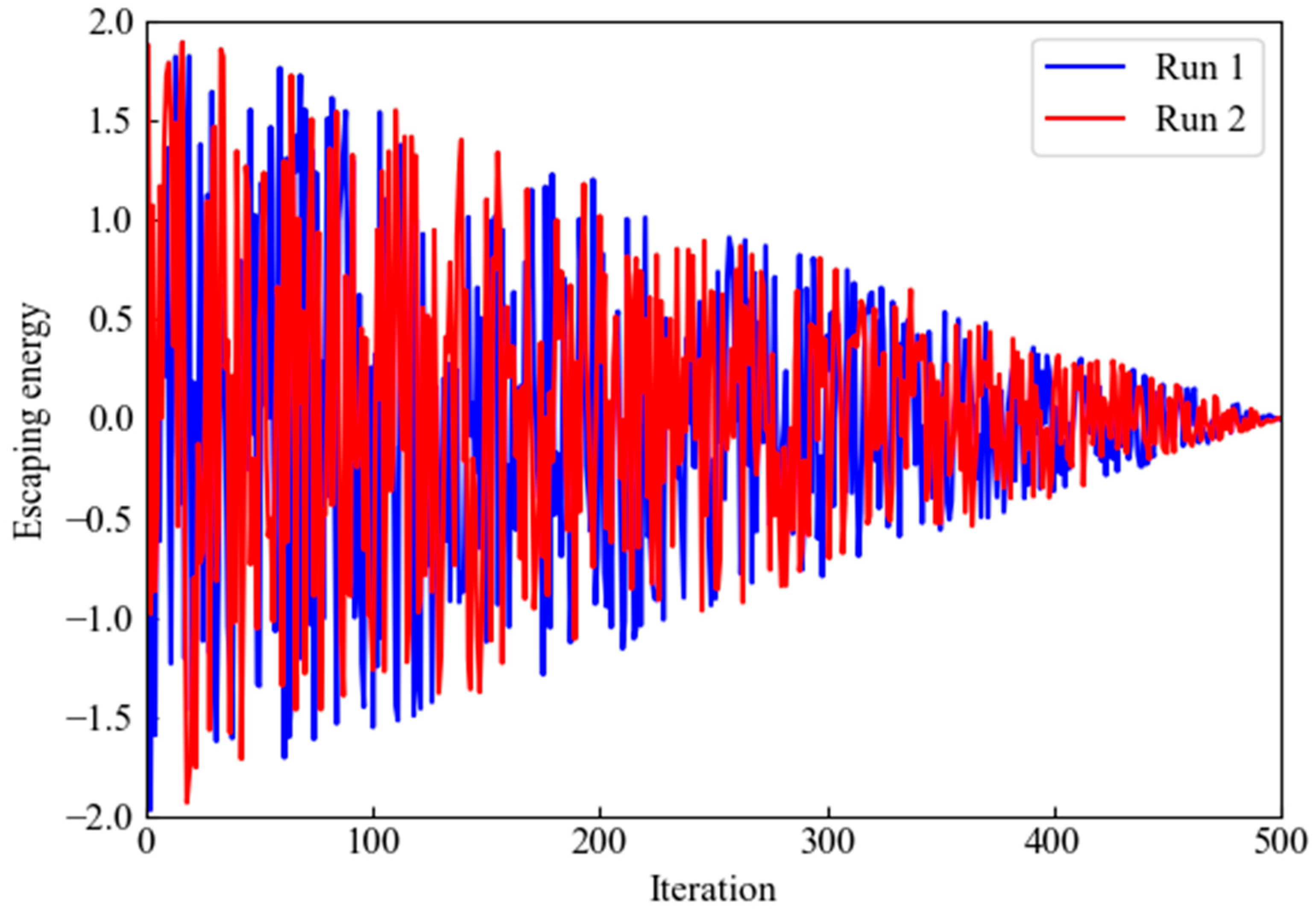
HHO’s transitions from exploration phase to exploitation phase are subject to the prey’s remaining escape energy. As the prey attempts to escape, its energy depletes significantly. The prey’s energy at the start, , fluctuates randomly in the range (−1, 1), while represents the escaping energy. The specific formula for describing this phenomenon is as follows:
here, represents maximum iteration count. Time-dependent behavior of is demonstrated in Figure 1.
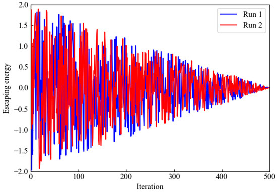
Figure 1.
Changes in across 2 runs and 500 iterations.
As shown in Figure 1, |E| must be less than 1 in the later iteration, resulting in unbalanced transition between the exploration and exploitation phases.
2.2.3. Exploitation Phase
HHO generates a random scalar within the range (0, 1) in this phase. The value of , in conjunction with the parameter , determines the update mechanism for the positions of Harris hawks. This update process is categorized into four distinct methods, as outlined in the following algorithm:
- (1)
- When r ≥ 0.5 and |E| ≥ 0.5, the formula used to update the location of the Harris hawk is the following:here, J is a value randomly chosen from the range (0, 2).
- (2)
- When r ≥ 0.5 and |E| < 0.5, the formula used to update the location of the Harris hawk is the following:
- (3)
- When r < 0.5 and |E| ≥ 0.5, the formula used to update the location of the Harris hawk is the following:here, is the dimensionality of the problem and is the stochastic generated vector. is a Levy flight strategy introduced to simulate the deceptive movements of a rabbit during the escape phase [26]. and are stochastic variables within the bounds of (0, 1). is assigned a default fixed value of 1.5.
- (4)
- When r < 0.5 and |E| < 0.5, the formula used to update the location of the Harris hawk is the following:
Through the prey’s escaping energy and random factors q and r, the HHO algorithm created multiple strategies for position updates. Then, it finally found the optimal solution in the search region by repeatedly adjusting the location of the Harris hawk.
2.3. Optimization of HHO Algorithm
2.3.1. Chaotic Mapping
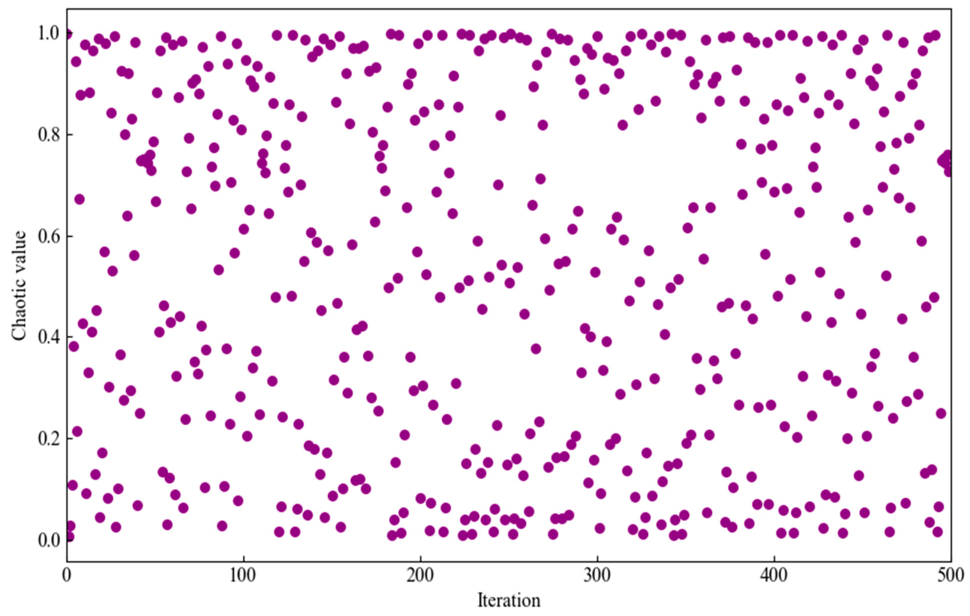
Chaos, a common nonlinear phenomenon in nature, is frequently utilized by researchers for optimizing search problems due to its inherent randomness, long-term unpredictability, and regularity. Experimental results have shown that chaotic mapping benefits optimization algorithms by maintaining population diversity, facilitating the evasion of local optima, as well as enhancing global search performance. One of the most commonly used chaotic maps is the logistic map, and its mathematical expression is as follows:
here, denotes the control parameter that dictates the behavior of the chaotic map. is a stochastic variable that lies within the bounds of 0 to 1. Experimental results indicate that when , the logistic map exhibits chaotic behavior; thus, is defined as 3.99 for the purposes of this research. The evolution of the logistic chaotic map values is shown in Figure 2.
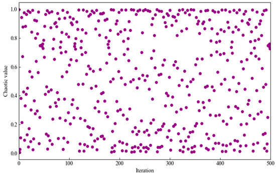
Figure 2.
Logistic map values over iterations.
2.3.2. Gaussian Mutation
Gaussian mutation, as an upgrade to the genetic algorithm, modifies the initial parameter by replacing it with a value randomly selected from a normal distribution with mean and variance . Mutation formula is shown as follows:
here, refers to the individual’s position post-mutation.
Given the properties of the Gaussian distribution, the main search region of Gaussian mutation is localized around the original entity. This method enhances both the algorithm’s robustness and its local search capability, thereby enabling the algorithm to efficiently locate the global minimum.
2.3.3. CHHO Algorithm
HHO relies on a linear decay method to change the escape energy factor, which leads to an imbalance in exploration and development and cannot accurately represent the actual multi-round hunting and escaping process between eagles and prey because |E| must be less than 1 in the later iterations; only local search is performed, so the search is not global; if the initial population is close to the local optimum, it may lead to the algorithm becoming trapped in a local extremum in later stages and unable to escape. A non-linear decay method can be used to dynamically adjust the algorithm parameters .
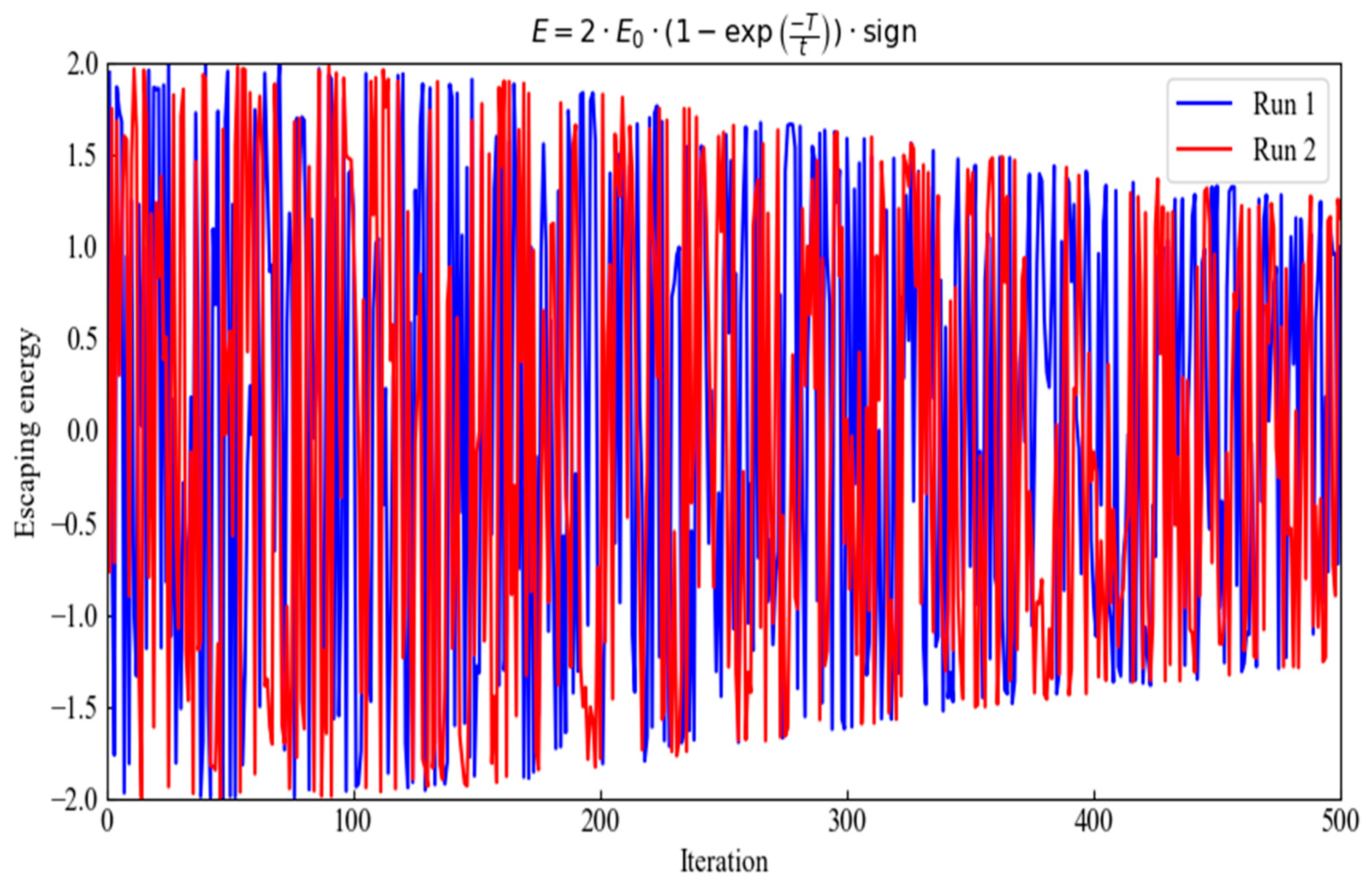
So, in this paper, chaotic mapping is employed to update the initial escape energy , and an exponential decay factor is utilized to update in the HHO algorithm, thereby ensuring sufficient population diversity during the global exploration phase. The updated formulas for and are provided below, and the variation in escape energy is illustrated in Figure 3.
here, is a random value of −1 or 1.
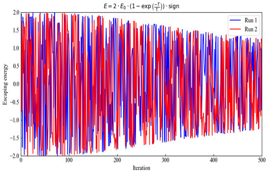
Figure 3.
Changes in new across 2 runs and 500 iterations.
As Figure 3 shows, compared to Figure 1, in the later iterations, the value of |E| fluctuates around 1 instead of remaining strictly below 1, achieving a balanced transition from the exploration phase to the exploitation phase.
The incorporation of the Gaussian mutation operator can significantly help the algorithm avoid being stuck in regional optima. In this paper, Gaussian mutation is applied to the current optimal solution with a specified probability (in this study ). Additionally, by referencing the concept of “greedy selection”, the selection rule based on the survival of the fittest is employed, and the following represents the update to the population’s position:
Figure 4 demonstrates the dynamic selection of VMD parameters through CHHO.
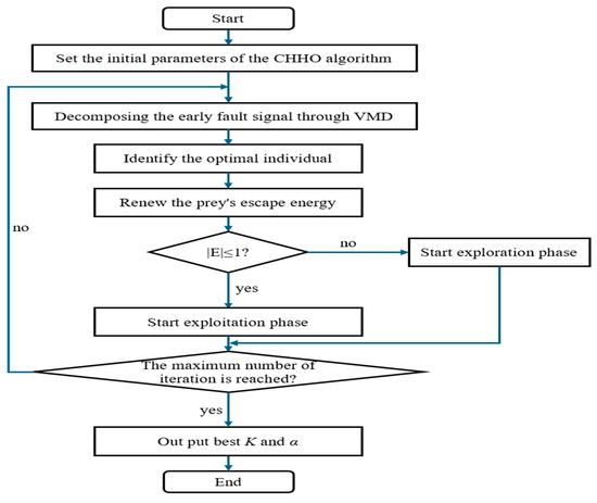
Figure 4.
Flowchart illustrating the adjustment of VMD parameters via CHHO technique.
2.4. Proposed Method
2.4.1. Selection of Fitness Function and Signal Reconstruction Index
A smaller energy entropy in a bearing signal containing a fault indicates that the vibration or shock signals caused by the fault are significant and concentrated, leading to periodic signal enhancement, making the fault characteristics more distinct. Therefore, this study uses the average minimum energy entropy as the iterative index in the optimization process, and the specific calculation formula is given below:
where is the component of the k-th IMF; denotes the average energy entropy of component ; represents the proportion of energy of the component in total energy; refers to the energy of the components; and indicates the cumulative energy of the components.
Kurtosis, a dimensionless metric, gauges sharpness or peak of a waveform and is particularly sensitive to impact signals. During bearing failure, the vibration signal generates a shock component, resulting in an elevation in the signal’s kurtosis value. Additionally, cross-correlation coefficient assesses the strength of correlation among signals. A higher correlation coefficient among IMF signal components indicates more sensitive information, whereas a lower coefficient suggests the presence of more additional disruptive components. Taking this into account, in processing rolling-bearing-fault signals, this study will apply both criteria to choose the signal components used for fault signal rebuilding. The formula for the two criteria is as follows:
here, and correspond to the signal’s mean and standard deviation, respectively, and stands for its expected value. represents the i-th data point’s value in the IMF component, with denoting the average of IMF component. Similarly, indicates the value associated with the i-th data point in the raw signal, where represents the mean of the raw signal.
2.4.2. Algorithmic Flow
According to the preceding analysis, and are key factors that significantly affect the VMD decomposition outcomes. Improper parameter selection can lead to modal component loss or mode aliasing. To overcome this challenge, this paper integrates CHHO algorithm into the VMD parameter optimization process, allowing for the adaptive selection of optimal parameters, thus eliminating the need for manual parameter setting derived from experience.
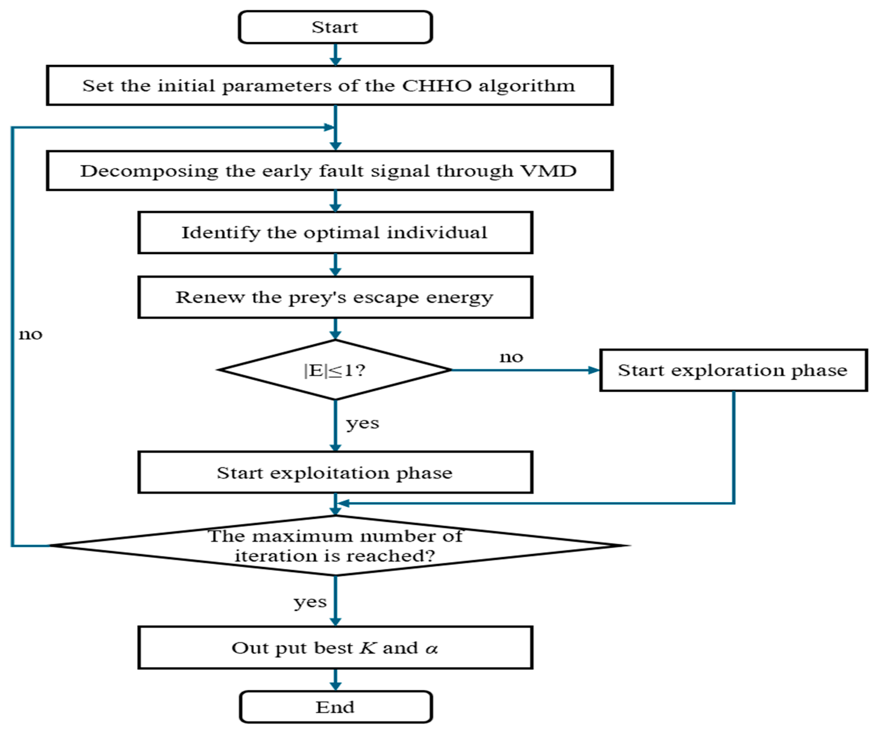
Therefore, this study adopts the minimum average energy entropy as its optimization goal, uses kurtosis value as evaluation criteria for selecting IMF components, and the CHHO algorithm is applied for the optimization of the VMD parameters [α, K]. This approach aims to effectively extract the bearing-fault characteristic frequencies. Figure 5 depicts the process, and specific steps are outlined below.
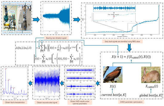
Figure 5.
Flowchart illustrating the early-fault feature extraction process with the CHHO–VMD.
Step 1: With the horizontal vibration signal, the CHHO algorithm was employed to adjust the VMD parameters adaptively, resulting in the optimal values for the parameter pair [, ]. In this study, the VMD algorithm’s two key parameters [α, K] were set to [400, 2] and [5000, 15], while the CHHO algorithm was configured with 50 sparrows in the population and a cap of 30 iterations.
Step 2: IMFs with a kurtosis value greater than 3 and cross-correlation coefficient exceeding 0.45 are selected for signal reconstruction.
Step 3: CHHO–VMD algorithm effectively extracted both the bearing rotation frequency and the early-fault characteristic frequencies.
3. Application
3.1. Early Weak Bearing-Fault Feature Frequency Extraction Using the IMS Bearing Dataset
3.1.1. IMS Bearing Dataset
Among the experimental datasets in this paper is the bearing dataset collected at the University of Cincinnati. A total of four identical bearing samples were evaluated in this dataset, and a sample exhibiting an outer-ring failure was specifically selected for this experiment in this paper. The rolling-bearing test rig, as depicted in Figure 6, utilizes Rexnord ZA-2115 bearings, which were sampled at 20 kHz and rotated at a frequency of 33.3 Hz. Further, the test rig possesses the following characteristics: a 6000-pound load is applied to the shaft and bearing via a spring mechanism, and PCB 253B33 high-sensitivity Quart accelerometers are utilized. A comprehensive list of the parameters is provided in Table 1.
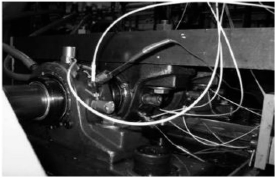
Figure 6.
Testbed of rolling-element bearings of Cincinnati University [27].

Table 1.
Parameters of bearings.
To compute the theoretical fault feature frequencies for the rolling bearings, the following formulas are used.
here, represents the bearing rotation frequency, denotes the quantity of rolling elements, refers to the rolling elements’ diameter, stands for the bearing mean diameter, and indicates the contact angle between the rolling elements.
Data from Table 1 are substituted into Formula (23) for calculation, yielding an outer-ring fault frequency of 236 Hz.
3.1.2. Extraction of Early-Fault Characteristic Frequency
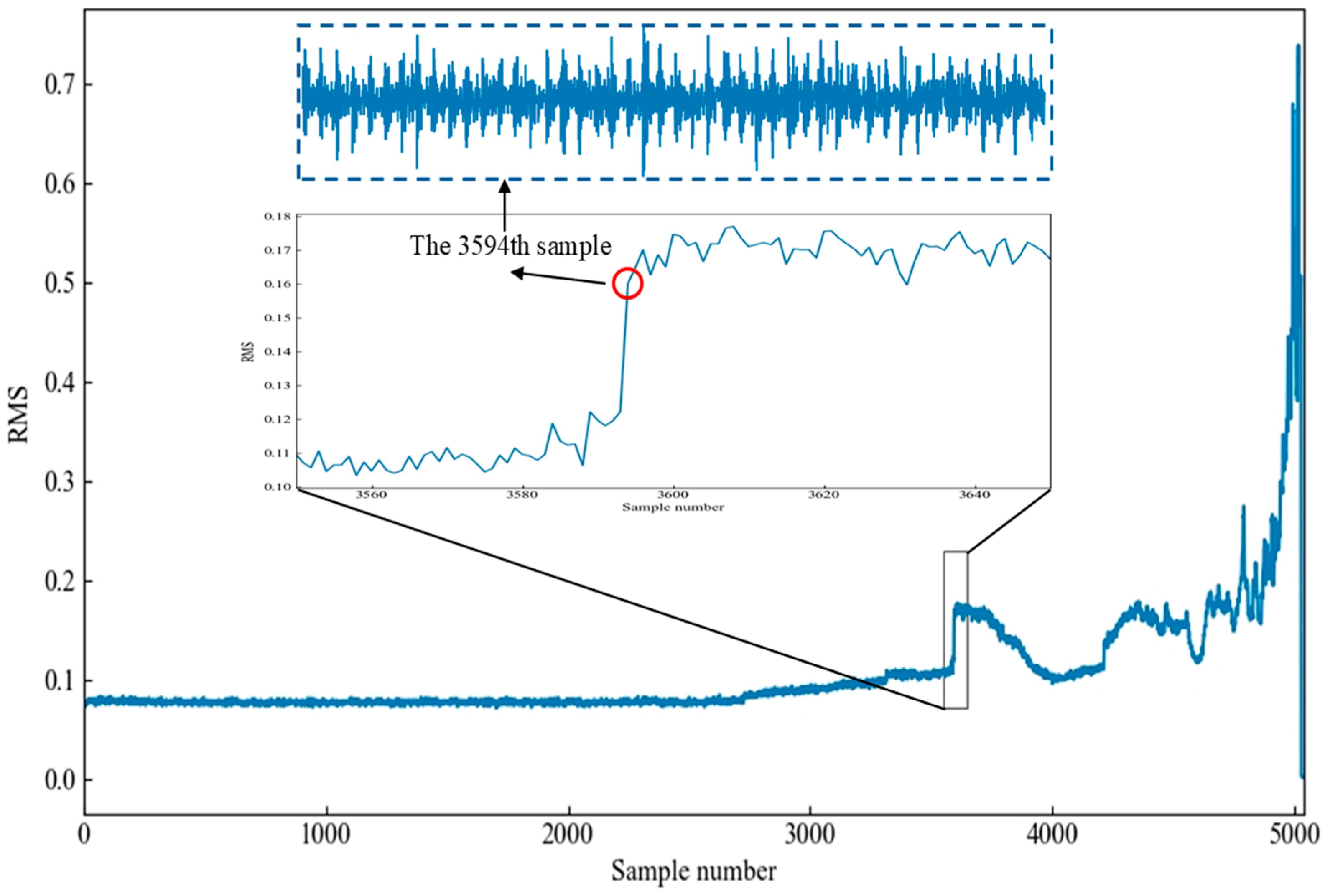
Early-fault signals within the original bearing vibration data are identified by utilizing the root mean square (RMS) value for analysis. RMS calculation is provided in Formula (24). A sample is formed by grouping 4000 (0.2 fs) points of the original vibration signal, with each sample’s RMS value plotted as the ordinate and the sample number as the abscissa to create Figure 7. As well, the extracted early-fault signal from the outer-ring bearing is highlighted within the blue dashed box in Figure 7.
here, represents the signal value of the i-th data point within a sample, while denotes the total count of signal points in the sample.

Figure 7.
Life chart of the outer-ring bearing using RMS value as the performance index and the results of early-fault signal extraction.
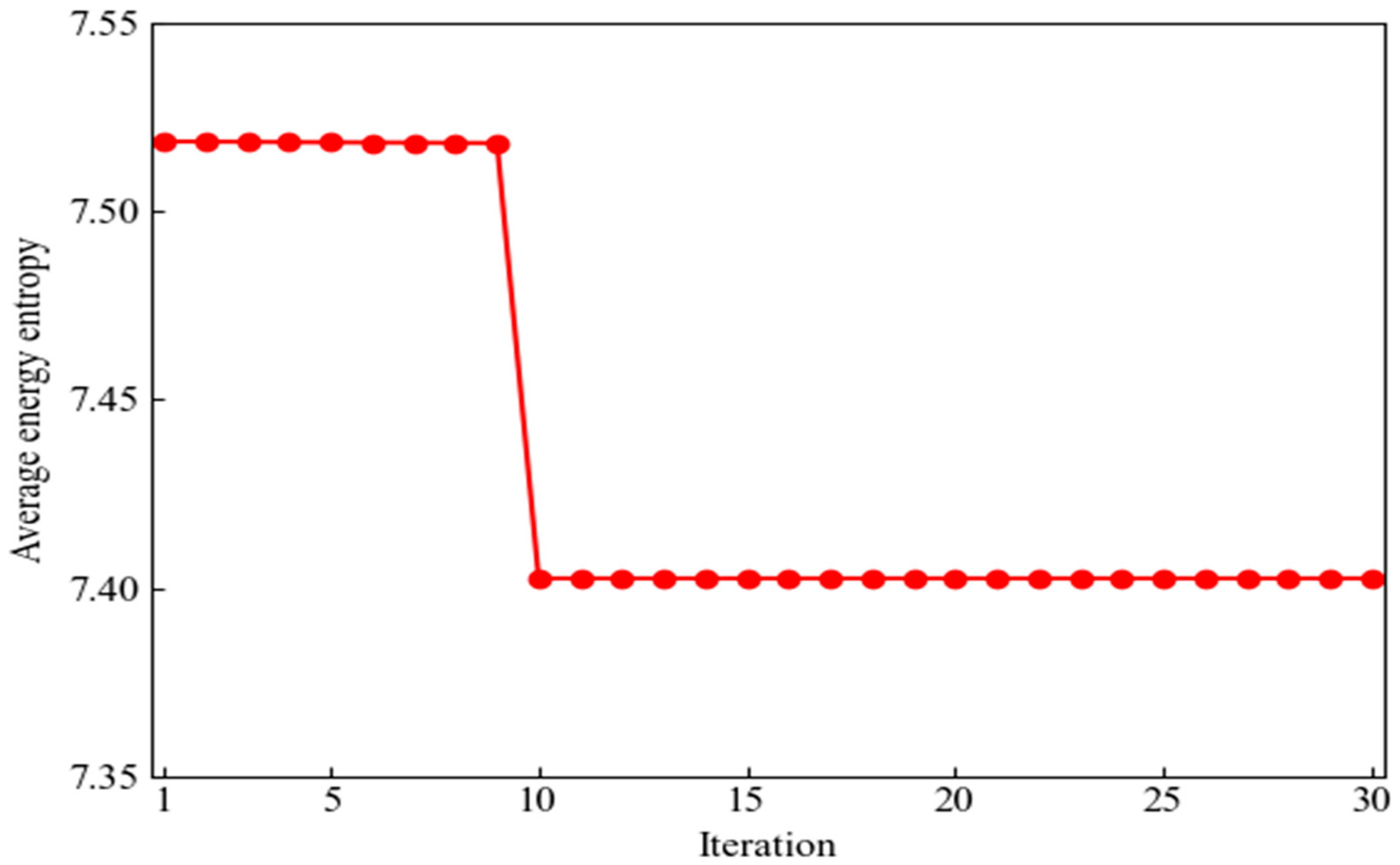
CHHO–VMD algorithm extracts early-fault features from the outer ring’s rolling-bearing-fault signals. Figure 8 depicts how the average energy entropy converges with increasing iterations during the adjustment of the VMD parameters.

Figure 8.
Convergence curve of the average energy entropy value during parameter optimization.
Optimal values for [K, α] were found to be [3, 400], resulting in minimum average energy entropy values of 7.4027, after CHHO optimization. The VMD decomposition results with these optimal parameters and the frequency domain diagram for each IMF are presented in Figure 9.
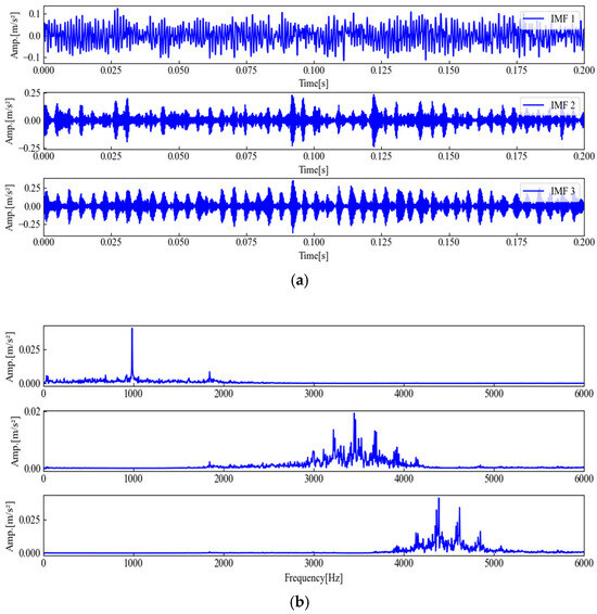
Figure 9.
Rolling-bearing vibration signal’s time-domain and spectrum plots after CHHO–VMD decomposition: (a) Temporal domain diagram; (b) Spectrum diagram.
The kurtosis and cross-correlation coefficient values for individual IMF are listed in Table 2.
Table 2.
The kurtosis and cross-correlation coefficient values for individual IMF.
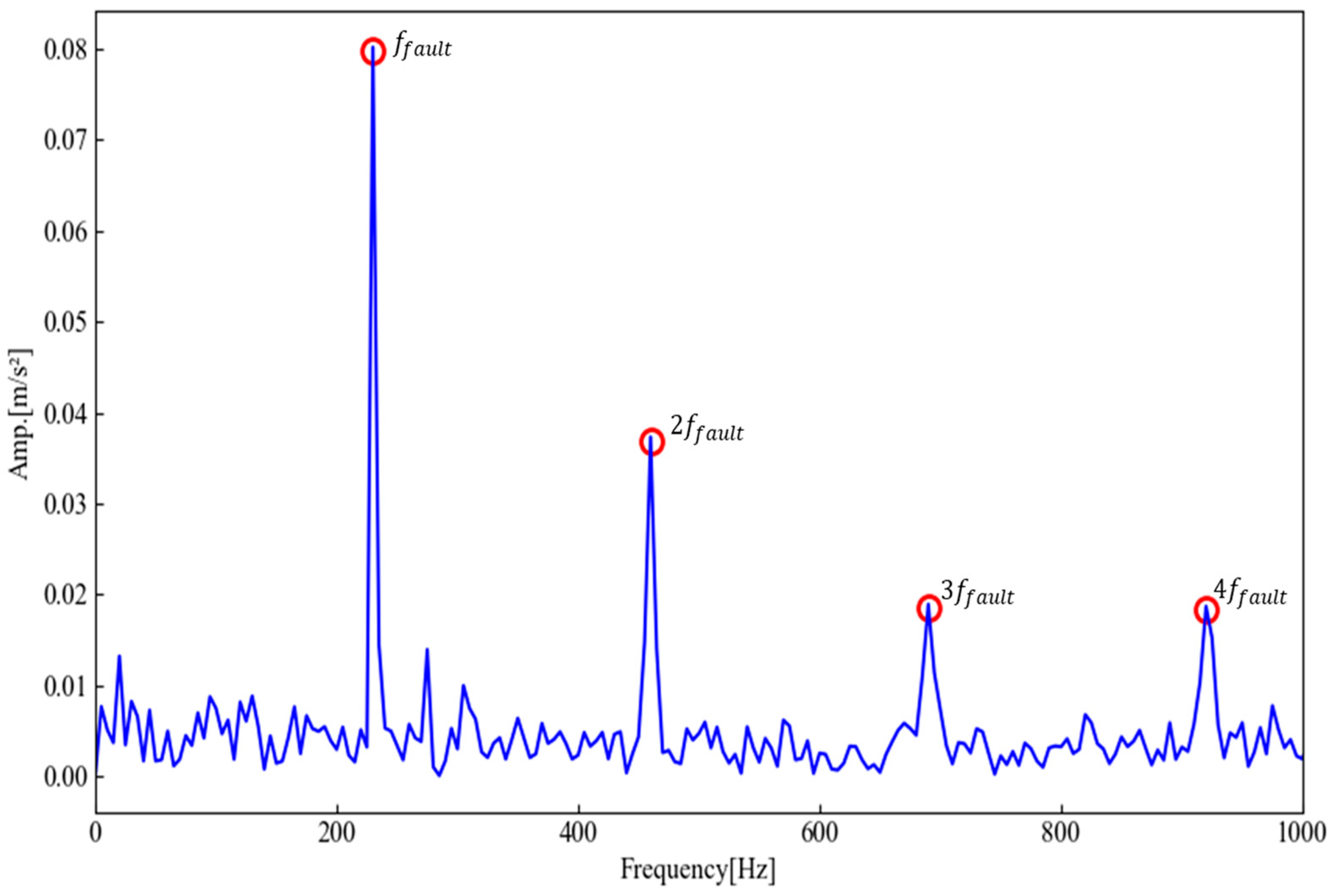
Based on kurtosis and correlation criteria, for the outer-ring results, both IMF2 and IMF3 are utilized in reconstructing the signal. Figure 10 shows the reconstructed signal’s envelope spectrum.
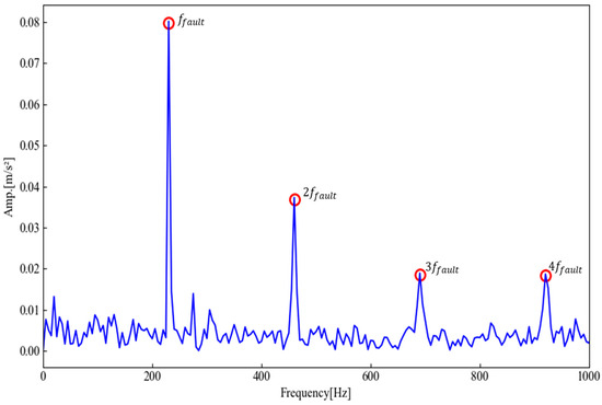
Figure 10.
Reconstructed signal’s envelope spectrum.
Figure 10 shows that the final envelope spectrum accurately extracts the early-fault characteristic frequency of the outer ring at 230 Hz, closely matching the theoretical value of 236 Hz.
3.2. Early Weak Bearing-Fault Characteristic Frequency Extraction Utilizing the Bearing Dataset of XJTU-SY
3.2.1. The XJTU-SY Bearing Dataset
One experimental dataset utilized in this paper is sourced from the XJTU-SY bearing dataset. Fifteen bearing samples were assessed in this dataset, with one showing outer-ring failure and another showing inner-ring failure selected for the experiment. The rolling-bearing test bed is shown in Figure 11, where two PCB 352C33 accelerometers are mounted at 90° on the bearing housing: one on the horizontal axis and the other on the vertical axis. The bearings tested are of type LDK UER204, and the sampling frequency was set to 25.6 kHz. Table 3 provides detailed parameters.
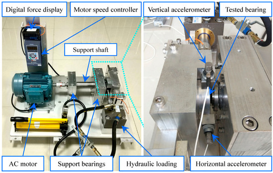
Figure 11.
Rolling element bearing test setup at Xi’an Jiaotong University [28].
Table 3.
Tested bearing parameters.
Table 4 lists the details of the two tested bearings used in this article, including bearing life and faulty components.
Table 4.
Data from the XJTU-SY bearing dataset employed in this research.
3.2.2. Extraction of Early-Fault Feature Frequency
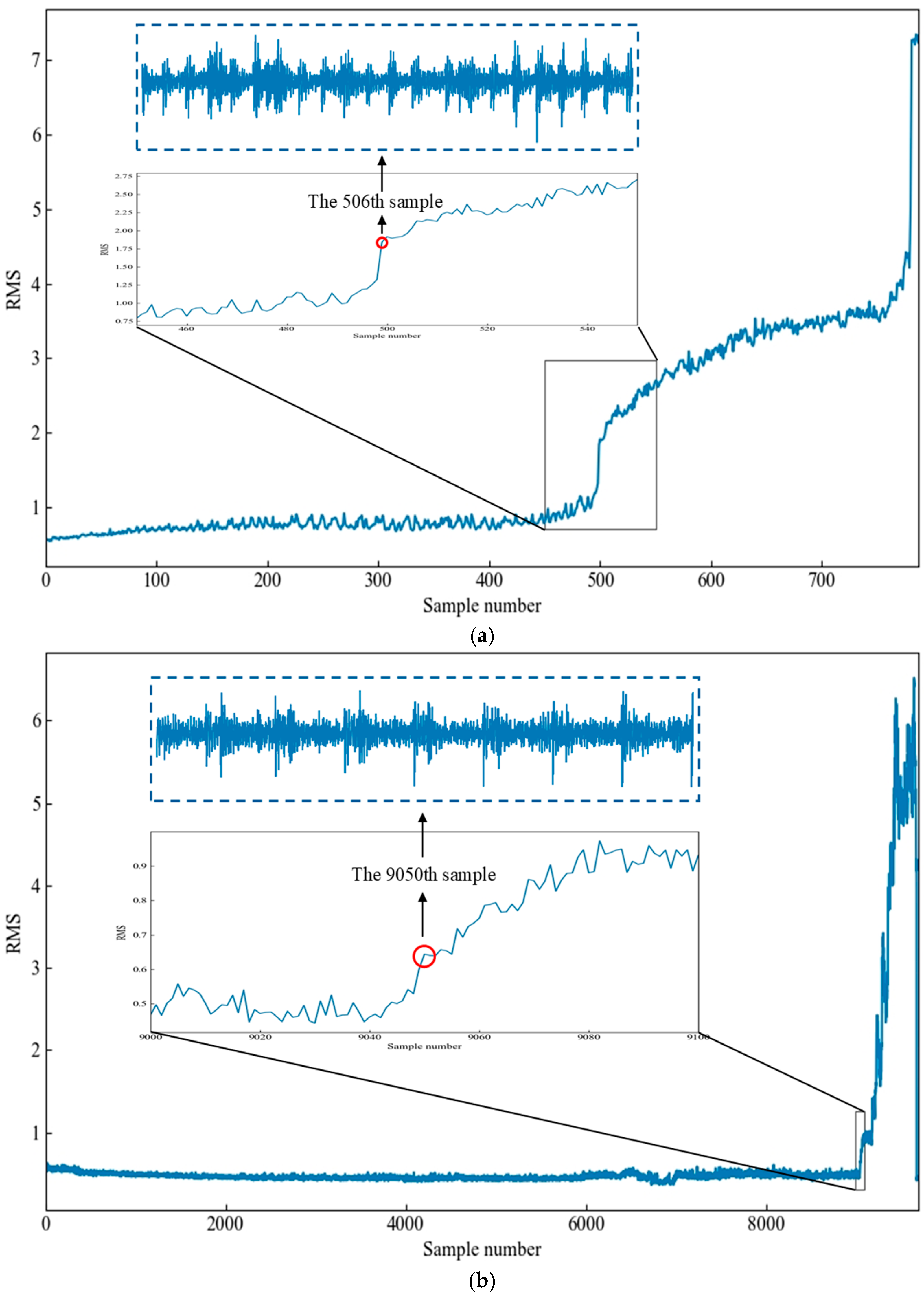
Similar to the first experiment, RMS value was used to detect early bearing-fault signals. Each sample was created by grouping 5120 (0.2 fs) points from the raw vibration signal, with RMS value as the ordinate and the sample count as the abscissa to form Figure 12. The early-fault signals extracted from the outer- and inner-ring bearings are highlighted within the blue dashed boxes in Figure 12, respectively.
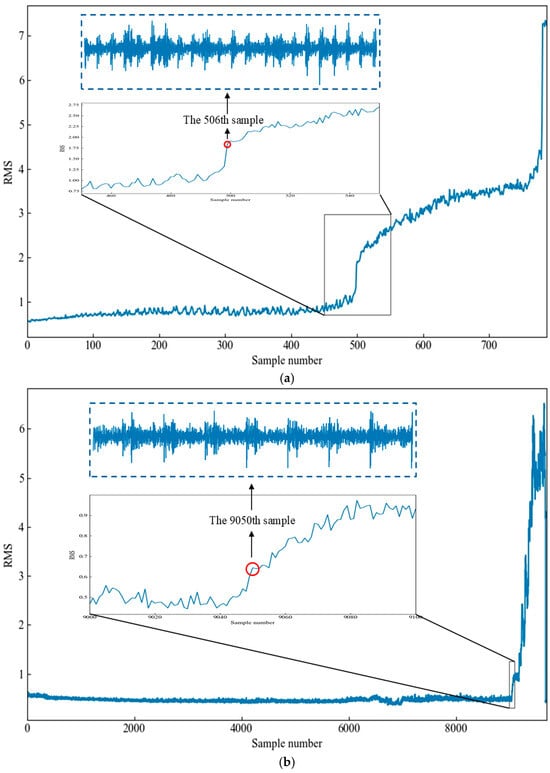
Figure 12.
Life chart of the outer and inner-ring bearings using the RMS value as the performance index and the results of early-fault signal extraction: (a) outer-ring bearing; (b) inner-ring bearing.
Figure 13 presents the spectrum diagram of the early-fault signals for both the inner- and outer-ring bearings. The fault signal, depicted above, is faint and comprises substantial noise frequencies. Characteristic frequencies of the fault states are not readily identifiable in the spectrum, thereby requiring further analysis. The application of the CHHO–VMD algorithm, introduced here, to extract fault features from rolling-bearing signals under real operating conditions is of critical importance.
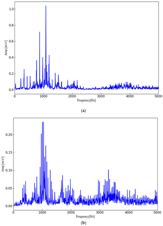
Figure 13.
Spectrum of rolling bearing: (a) outer-ring failure signal; (b) inner-ring failure signal.
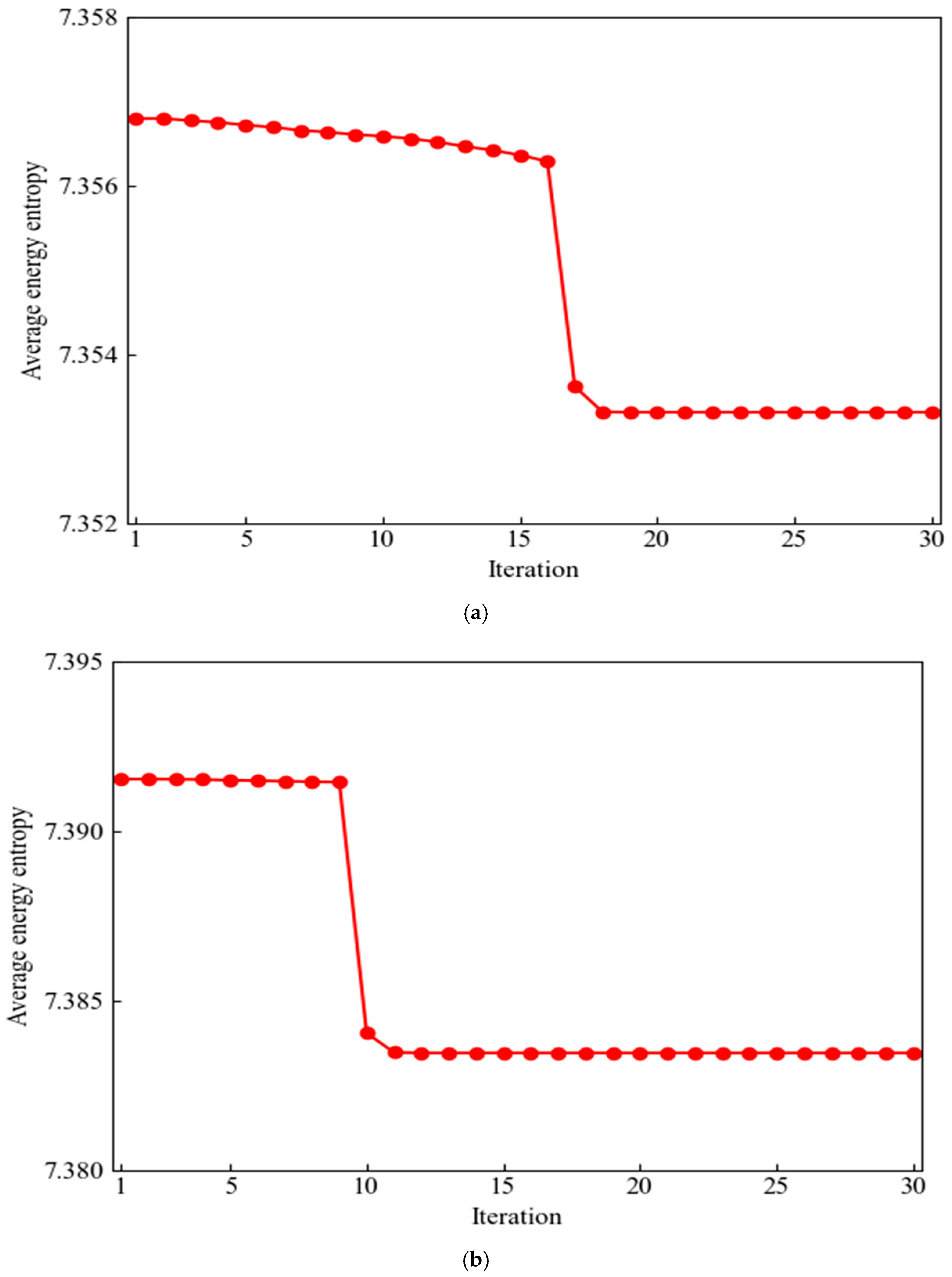
In this experiment, the CHHO–VMD algorithm is employed to extract early-fault characteristics from inner- and outer-ring rolling-bearing faults. Figure 14 illustrates the convergence curve of the average energy entropy concerning the number of iterations during the VMD parameter optimization procedure.
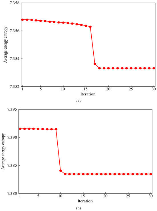
Figure 14.
Convergence curve of average energy entropy during VMD parameter optimization: (a) Outer-ring failure signal; (b) Inner-ring failure signal.
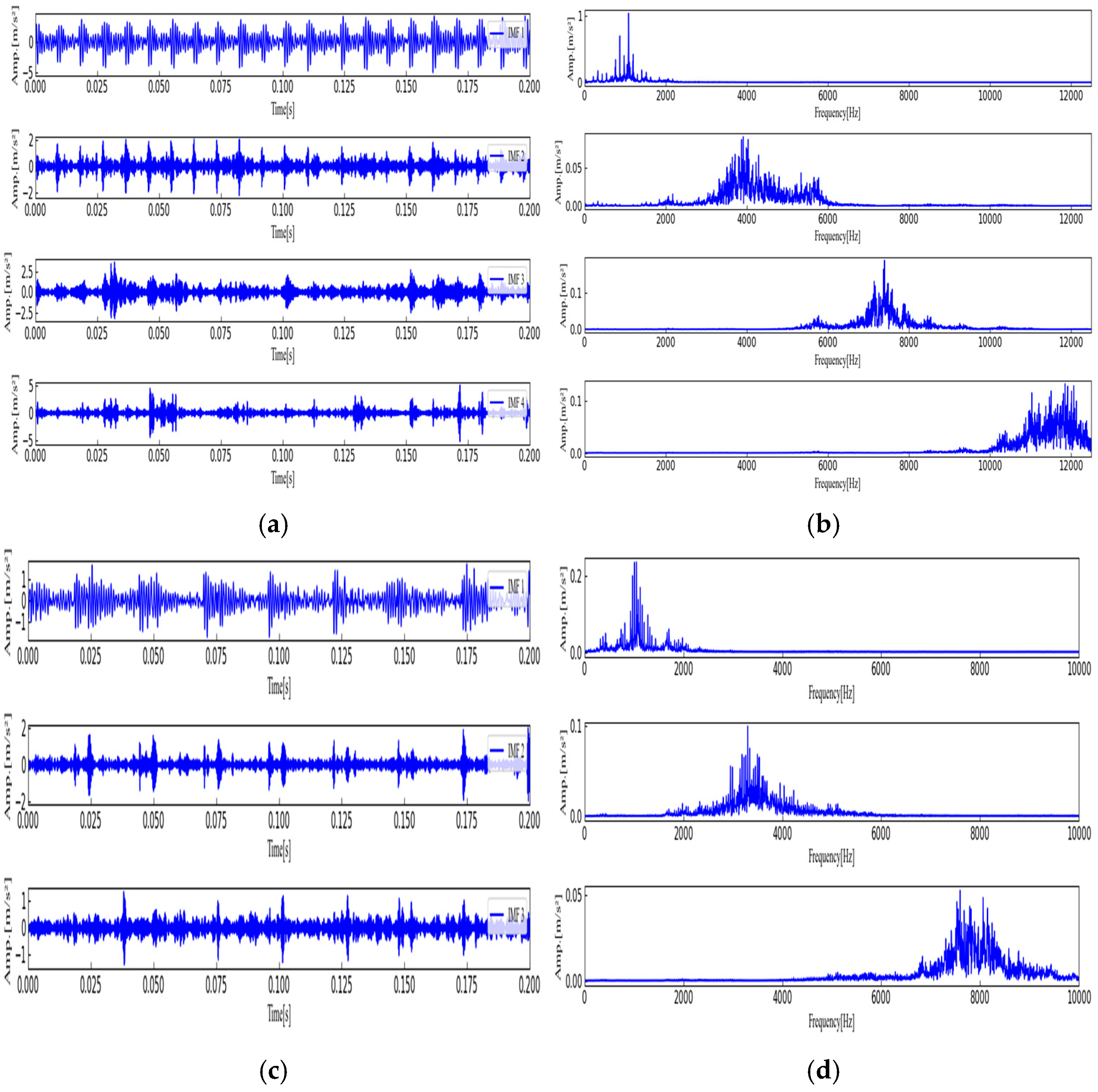
Optimal values for [K, α] were found to be [4, 550] and [3, 549], resulting in minimum average energy entropy values of 7.3533 and 7.3835, respectively, after CHHO optimization. Figure 15 illustrates the early-fault signals of the bearing, after applying the optimal parameter settings. From Figure 15, the modal components appear evenly spread across the frequency bands, without mode confusion, suggesting the signal is neither under-decomposed nor over-decomposed.
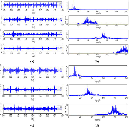
Figure 15.
Rolling-bearing vibration signal’s time-domain and spectrum plots after CHHO–VMD decomposition: (a) Outer-rolling-bearing signal in the temporal domain; (b) Outer-rolling-bearing signal in the spectrum; (c) Inner-rolling-bearing signal in the temporal domain; (d) Inner-rolling-bearing signal in the spectrum.
Table 5 shows the kurtosis and cross-correlation coefficient values of individual IMF components.
Table 5.
The kurtosis and cross-correlation coefficient values of individual IMF.
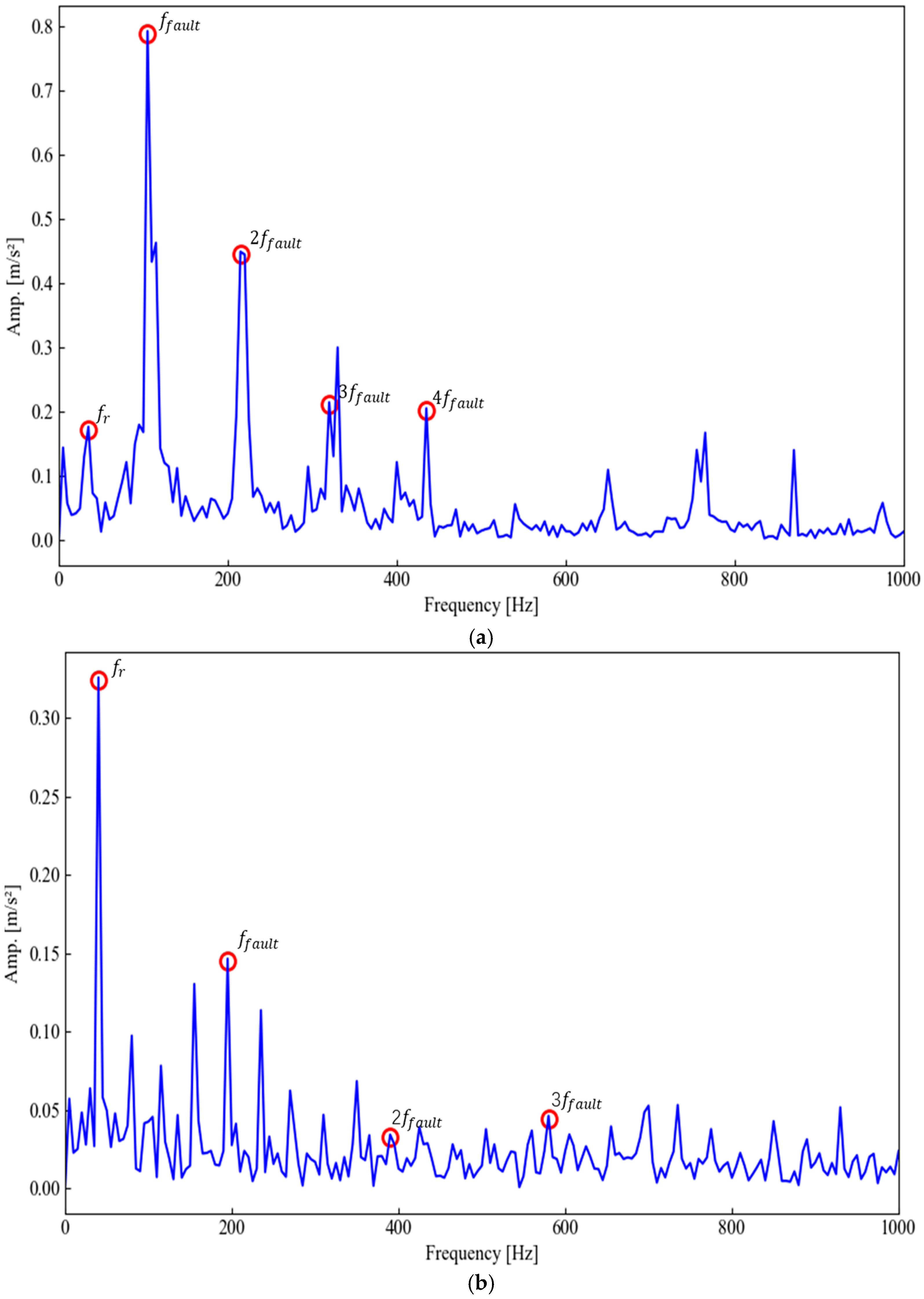
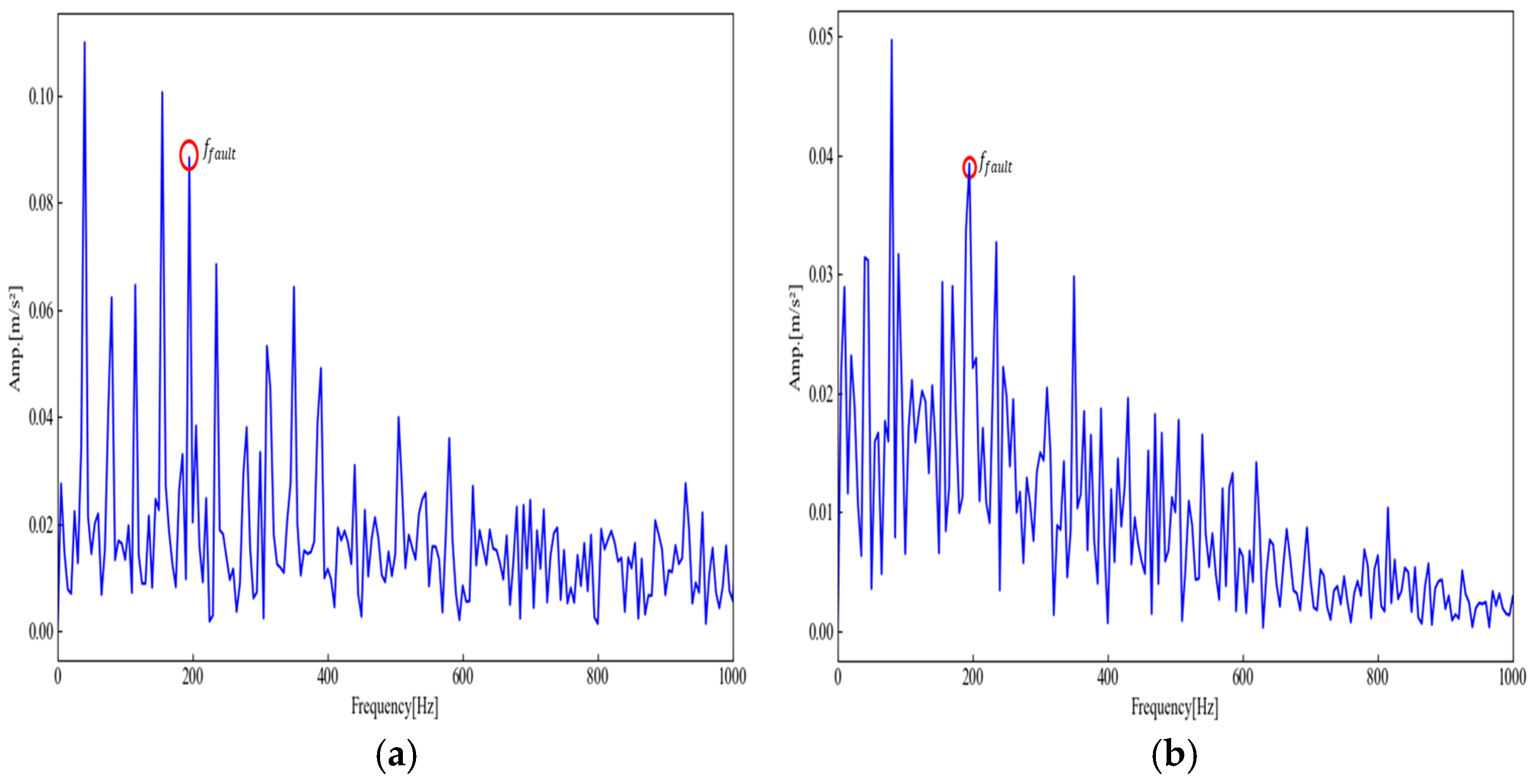
Based on kurtosis and correlation criteria, IMF1 was chosen to reconstruct the signal for the bearing’s outer rings. For the inner rings of the bearing, both IMF1 and IMF2 were selected for signal reconstruction. Figure 16 shows the reconstructed signal’s envelope spectrum.
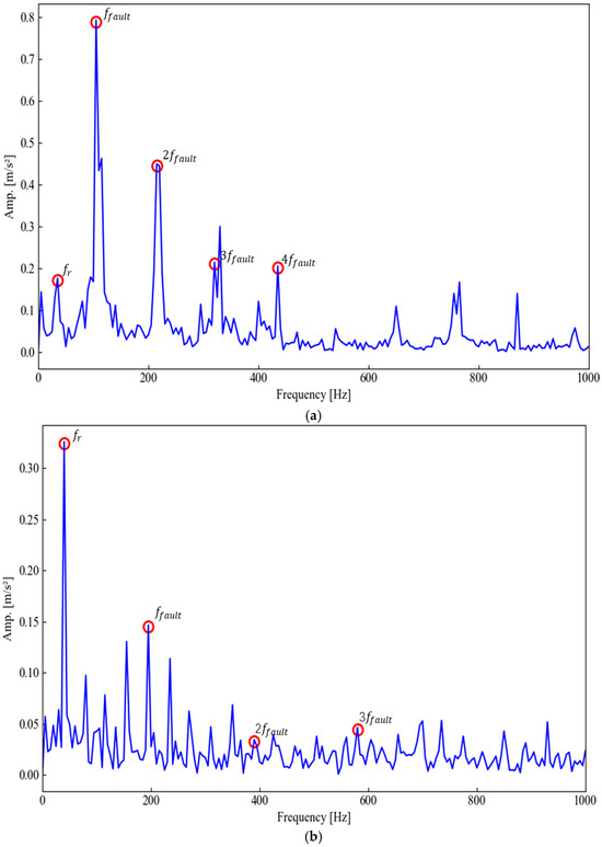
Figure 16.
Envelope spectrum corresponding to the reconstructed signal: (a) Bearing having outer race failure; (b) Bearing having inner race failure.
The analysis of Figure 16 reveals that the final envelope spectrum successfully extracts both the rotation frequency and fault feature frequency of the early-fault signal across both the outer and inner rings. At 35 Hz, the outer ring of the bearing rotates, while the inner-ring bearing rotates at 40 Hz. Figure 16 illustrates that the early-fault feature frequencies of both outer and inner-ring bearings are 110 Hz and 195 Hz, respectively, closely matching their theoretical values of 107.3 Hz and 196.9 Hz. Additionally, the frequency doubling of the fault feature for both outer and inner rings of the bearing is effectively extracted. It is evident that CHHO–VMD algorithm proves effective in addressing the challenge of extracting the characteristic frequency of early bearing faults to some degree.
To compare the CHHO–VMD algorithm with other methods, the EEMD, Fixed parameter VMD, PSO–VMD and ACO–VMD algorithms were employed to analyze the data from both outer and inner-ring rolling bearings in experiment 2. The envelope spectrum of the outer and inner-ring faults in the rolling bearing vibration signal, derived from different algorithms, is shown in Figure 17 and Figure 18: (a) EEMD algorithm, (b) Fixed parameter VMD algorithm (c) PSO–VMD algorithm, (d) ACO–VMD algorithm.
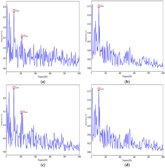
Figure 17.
Envelope spectra of the reconstructed outer-ring-bearing signals extracted using different methods (a) EEMD; (b)Fixed parameter VMD; (c) PSO–VMD; (d) ACO–VMD.
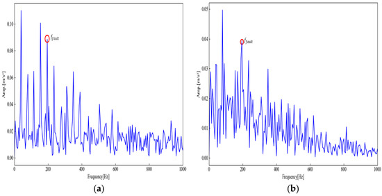
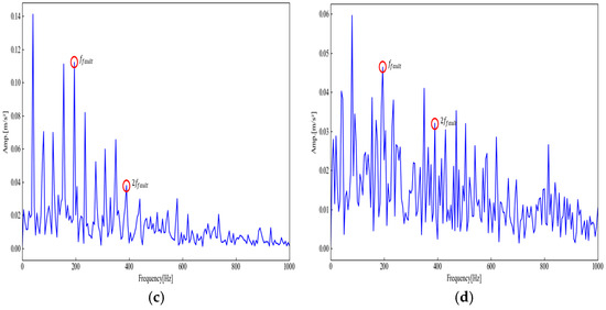
Figure 18.
Envelope spectra of the reconstructed inner-ring-bearing signals extracted using different methods (a) EEMD; (b)Fixed parameter VMD; (c) PSO–VMD; (d) ACO–VMD.
Comparisons of the envelope spectra in Figure 16a and Figure 17, as well as Figure 16b and Figure 18, reveal that these five algorithms are limited in extracting fault characteristic frequencies. Excessive noise in the spectra leads to identification inaccuracies, hindering harmonic frequency extraction. The signal decomposition results of the EEMD algorithm are highly unstable, with harmonic frequencies in the extracted correlation envelope spectrum being completely obscured by noise. Additionally, the algorithm lacks a solid mathematical basis. Selecting reasonable parameters for a fixed-parameter VMD algorithm is challenging; thus, the envelope spectrum extracted without parameter optimization is often unsatisfactory and contains significant noise. PSO and ACO are recent intelligent optimization algorithms with strong parameter optimization capabilities. However, they often fall into local optima and exhibit sluggish convergence. When combined with VMD, these algorithms can extract the fault feature frequency, but the envelope spectrum still contains substantial noise. In contrast, the CHHO algorithm can extract the bearing rotation frequency, outer-ring fault feature frequency, and their harmonics.
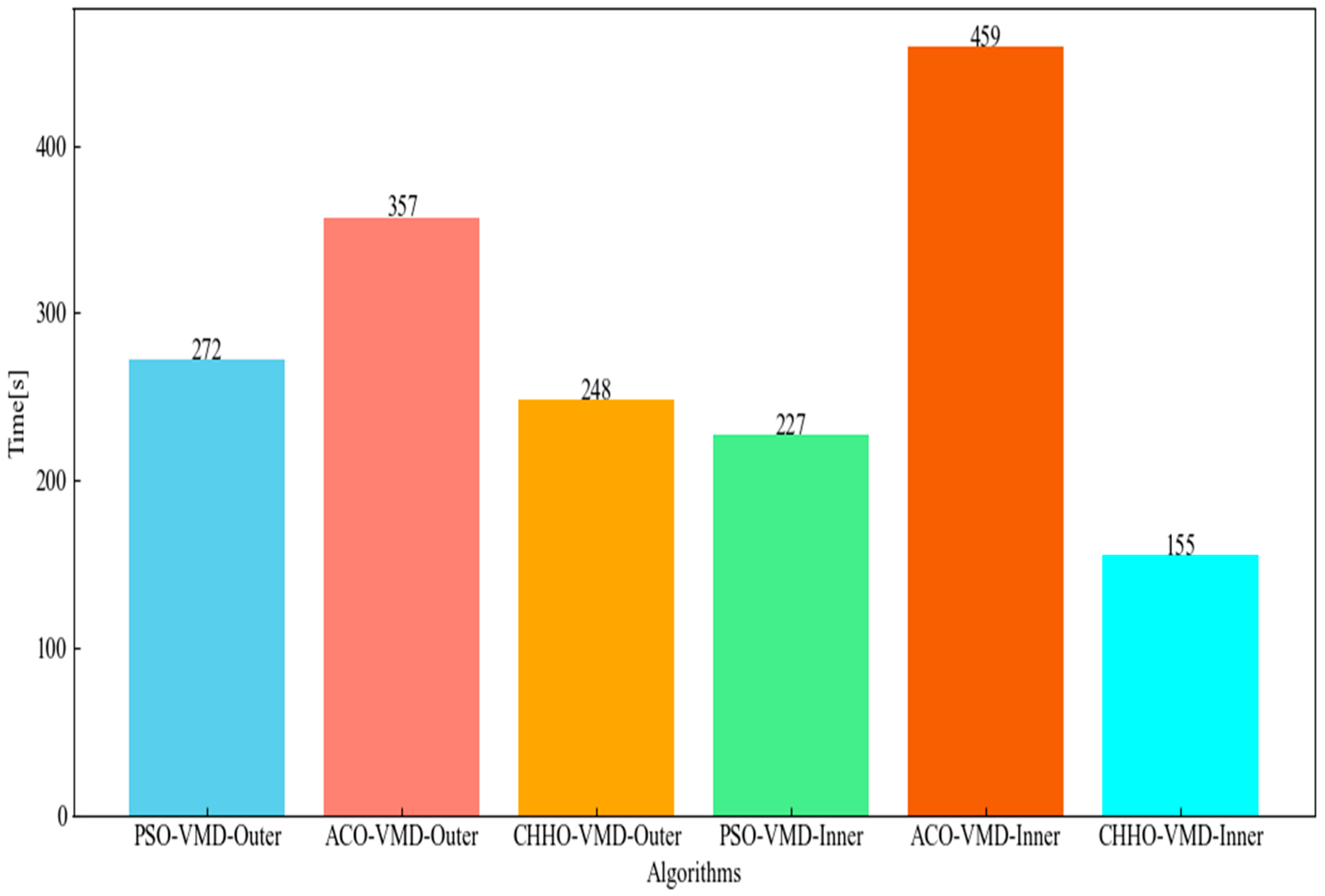
To further validate the CHHO algorithm’s fast convergence and ability to avoid local optima, the time consumption for completing the identical optimization task by three algorithms is shown in Figure 19.

Figure 19.
Time taken by different optimization algorithms to complete VMD parameter optimization tasks.
As shown in Figure 19, the CHHO–VMD algorithm converges faster and more accurately than the PSO–VMD and ACO–VMD algorithms. Based on prior experimental findings, the CHHO algorithm exhibits enhanced computational efficiency, a reduced likelihood of converging to local optima, and a more effective global search capability.
4. Conclusions
This paper introduces a novel technique for early-fault characteristics extraction in rolling bearings using CHHO–VMD. The method substantially enhances the precision of VMD signal decomposition by reframing the signal decomposition task as a parameter optimization problem. It tackles the issue of weak and challenging early-fault feature extraction in rolling bearings. At the outset, the method employs minimum average energy entropy with its objective function, the Chaotic Harris Hawk Optimization, to determine the best VMD parameters, effectively mitigating the impact of improper parameter selection. Based on kurtosis and cross-correlation coefficient, a dual rule is introduced to choose the appropriate components of the early-fault signal, enabling the reconstructed signal to reduce interference while preserving crucial fault information. Finally, envelope spectrum analysis successfully extracts the rotational frequency and the early-fault feature frequencies. The effectiveness of this method is confirmed through two experiments involving rolling bearings.
However, the CHHO algorithm still depends on several control parameters. Improper parameter settings may lead to unstable algorithm performance. And the effect of early-fault characteristic frequency extraction for inner-ring rolling bearings is not as efficient as that for the outer ring. Moreover, the fault extraction approach developed can be employed to evaluate wear severity in various forms of rotating machinery, extending the engineering implications and practical uses of this research. For future scientific research, researchers can explore further optimization of the CHHO algorithm to enhance both the speed and accuracy of parameter optimization in the VMD algorithm. Additionally, more rolling-bearing data can be collected from complex and extreme environments, and the CHHO–VMD algorithm can be applied to extract early-fault characteristic frequencies, further verifying the effectiveness of the algorithm.
Author Contributions
Conceptualization, J.N.; funding acquisition, G.H.; investigation, J.Y.; project administration, J.F.; software, J.N.; supervision, G.H.; validation, N.W.; writing—original draft, J.N.; writing—review & editing, J.N. All authors have read and agreed to the published version of the manuscript.
Funding
This research was funded by Sichuan Civil Aviation Flight Technology and Flight Safety Engineering Technology Research Center Project (No. GY2024-41E).
Data Availability Statement
The raw data supporting the conclusions of this article will be made available by the authors on request.
Conflicts of Interest
The authors declare no conflicts of interest.
References
- Pastukhov, A.; Timashov, E.; Stanojević, D. Temperature Conditions and Diagnostics of Bearings. Appl. Eng. Lett. J. Eng. Appl. Sci. 2023, 8, 45–51. [Google Scholar] [CrossRef]
- Desnica, E.; Ašonja, A.; Radovanović, L.; Palinkaš, I.; Kiss, I. Selection, dimensioning and maintenance of roller bearings. In Proceedings of the International Conference on Organization and Technology of Maintenance 2022, Osijek, Croatia, 29–30 November 2022; Springer International Publishing: Cham, Swizterland, 2022; pp. 133–142. [Google Scholar]
- Liu, X.; He, Y.; Wang, L. Adaptive transfer learning based on a two-stream densely connected residual shrinkage network for transformer fault diagnosis over vibration signals. Electronics 2021, 10, 2130. [Google Scholar] [CrossRef]
- Li, Y.; Wang, S.; Deng, Z. Intelligent fault identification of rotary machinery using refined composite multi-scale Lempel–Ziv complexity. J. Manuf. Syst. 2021, 61, 725–735. [Google Scholar] [CrossRef]
- Li, Y.; Wang, X.; Liu, Z.; Liang, X.; Si, S. The entropy algorithm and its variants in the fault diagnosis of rotating machinery: A review. IEEE Access 2018, 6, 66723–66741. [Google Scholar] [CrossRef]
- Smith, J.S. The local mean decomposition and its application to EEG perception data. J. R. Soc. Interface 2005, 2, 443–454. [Google Scholar] [CrossRef]
- Kankar, P.K.; Sharma, S.C.; Harsha, S.P. Fault diagnosis of ball bearings using continuous wavelet transform. Appl. Soft Comput. 2011, 11, 2300–2312. [Google Scholar] [CrossRef]
- Huang, N.E.; Shen, Z.; Long, S.R.; Wu, M.C.; Shih, H.H.; Zheng, Q.; Yen, N.C.; Tung, C.C.; Liu, H.H. The empirical mode decomposition and the Hilbert spectrum for nonlinear and non-stationary time series analysis. Proc. R. Soc. Lond. Ser. A Math. Phys. Eng. Sci. 1998, 454, 903–995. [Google Scholar] [CrossRef]
- Wu, Z.; Huang, N.E. Ensemble empirical mode decomposition: A noise-assisted data analysis method. Adv. Adapt. Data Anal. 2009, 1, 1–41. [Google Scholar] [CrossRef]
- Torres, M.E.; Colominas, M.A.; Schlotthauer, G.; Flandrin, P. A complete ensemble empirical mode decomposition with adaptive noise. In Proceedings of the 2011 IEEE International Conference on Acoustics, Speech and Signal Processing (ICASSP) 2011, Prague, Czech Republic, 22–27 May 2011; p. 41444147. [Google Scholar]
- Zhen, D.; Li, D.; Feng, G.; Zhang, H.; Gu, F. Rolling bearing fault diagnosis based on VMD reconstruction and DCS demodulation. Int. J. Hydromechatronics 2022, 5, 205–225. [Google Scholar] [CrossRef]
- Dragomiretskiy, K.; Zosso, D. Variational mode decomposition. IEEE Trans. Signal Process. 2013, 62, 531–544. [Google Scholar] [CrossRef]
- Li, H.; Fan, B.; Jia, R.; Zhai, F.; Bai, L.; Luo, X. Research on multi-domain fault diagnosis of gearbox of wind turbine based on adaptive variational mode decomposition and extreme learning machine algorithms. Energies 2020, 13, 1375. [Google Scholar] [CrossRef]
- Deng, W.; Liu, H.; Zhang, S.; Liu, H.; Zhao, H.; Wu, J. Research on an adaptive variational mode decomposition with double thresholds for feature extraction. Symmetry 2018, 10, 684. [Google Scholar] [CrossRef]
- Ding, J.; Huang, L.; Xiao, D.; Li, X. GMPSO-VMD algorithm and its application to rolling bearing fault feature extraction. Sensors 2020, 20, 1946. [Google Scholar] [CrossRef] [PubMed]
- Li, Y.; Tang, B.; Jiang, X.; Yi, Y. Bearing fault feature extraction method based on GA-VMD and center frequency. Math. Probl. Eng. 2022, 2022, 2058258. [Google Scholar] [CrossRef]
- Lv, M.; Liu, S.; Chen, C. A new feature extraction technique for early degeneration detection of rolling bearings. IEEE Access 2022, 10, 23659–23676. [Google Scholar] [CrossRef]
- Mirjalili, S.; Mirjalili, S.M.; Lewis, A. Grey wolf optimizer. Adv. Eng. Softw. 2014, 69, 46–61. [Google Scholar] [CrossRef]
- Liu, Z.; Li, S.; Wang, R.; Jia, X. Research on Fault Feature Extraction Method of Rolling Bearing Based on SSA–VMD–MCKD. Electronics 2022, 11, 3404. [Google Scholar] [CrossRef]
- Wang, H.D.; Deng, S.E.; Yang, J.X.; Liao, H.; Li, W.B. Parameter-Adaptive VMD Method Based on BAS Optimization Algorithm for Incipient Bearing Fault Diagnosis. Math. Probl. Eng. 2020, 2020, 5659618. [Google Scholar] [CrossRef]
- Jin, Z.; He, D.; Lao, Z.; Wei, Z.; Yin, X.; Yang, W. Early intelligent fault diagnosis of rotating machinery based on IWOA-VMD and DMKELM. Nonlinear Dyn. 2023, 111, 5287–5306. [Google Scholar] [CrossRef]
- Heidari, A.A.; Mirjalili, S.; Faris, H.; Aljarah, I.; Mafarja, M.; Chen, H. Harris hawks optimization: Algorithm and applications. Future Gener. Comput. Syst. 2019, 97, 849–872. [Google Scholar] [CrossRef]
- Gezici, H.; Livatyalı, H. Chaotic Harris hawks optimization algorithm. J. Comput. Des. Eng. 2022, 9, 216–245. [Google Scholar] [CrossRef]
- Ibrahim, A.; Ali, H.A.; Eid, M.M.; El-kenawy, E.S. Chaotic harris hawks optimization for unconstrained function optimization. In Proceedings of the 2020 16th International Computer Engineering Conference (ICENCO), Cairo, Egypt, 29–30 December 2020; pp. 153–158. [Google Scholar]
- Dhawale, D.; Kamboj, V.K.; Anand, P. An improved Chaotic Harris Hawks Optimizer for solving numerical and engineering optimization problems. Eng. Comput. 2023, 39, 1183–1228. [Google Scholar] [CrossRef]
- Yang, X.S. Nature-Inspired Metaheuristic Algorithms; Luniver Press: Bristol, UK, 2010. [Google Scholar]
- Gousseau, W.; Antoni, J.; Girardin, F.; Griffaton, J. Analysis of the Rolling Element Bearing data set of the Center for Intelligent Maintenance Systems of the University of Cincinnati. CM2016 10 October 2016. Available online: https://hal.science/hal-01715193/ (accessed on 15 December 2024).
- Wang, B.; Lei, Y.; Li, N.; Li, N. A hybrid prognostics approach for estimating remaining useful life of rolling element bearings. IEEE Trans. Reliab. 2018, 69, 401–412. [Google Scholar] [CrossRef]


Disclaimer/Publisher’s Note: The statements, opinions and data contained in all publications are solely those of the individual author(s) and contributor(s) and not of MDPI and/or the editor(s). MDPI and/or the editor(s) disclaim responsibility for any injury to people or property resulting from any ideas, methods, instructions or products referred to in the content. |
© 2025 by the authors. Licensee MDPI, Basel, Switzerland. This article is an open access article distributed under the terms and conditions of the Creative Commons Attribution (CC BY) license (https://creativecommons.org/licenses/by/4.0/).