Article

The Application of Recurrence Plots to Identify Nonlinear Responses Using Magnetometer Data for Wind Turbine Design

by
Juan Carlos Jauregui-Correa
* and
Luis Morales-Velazquez
Facultad de Ingeniería, Universidad Autónoma de Querétaro, Cerro de las Campanas S/N, Col. las Campanas, Santiago de Querétaro 76010, Mexico
*
Author to whom correspondence should be addressed.
Machines 2025, 13(3), 233; https://doi.org/10.3390/machines13030233
Submission received: 27 January 2025 / Revised: 9 March 2025 / Accepted: 10 March 2025 / Published: 13 March 2025
(This article belongs to the Special Issue Nonlinear Mechanical Vibration in Machine Design)

Abstract

:
This work uses recurrence plots (RPs) to identify nonlinearities and non-stationary conditions in wind turbines. Traditionally, recurrence plots have been applied to vibration or acoustic data; this paper applies them to magnetometer and accelerometer data to compare the sensitivity. The recurrence plots are generated by plotting points in the phase space and identifying those points where the dynamic system returns to a similar configuration, meaning that the state variables are similar to previous conditions. The state variables for the acceleration data are the position and velocity, whereas, for the magnetometer data, they are the magnitude of the magnetic field and its integral. The time series are integrated by combining the shifting principle of harmonic functions and the empirical mode decomposition. The EMD method separates the original signal into several modes, shifts them, and combines them back. The time series were obtained from an accelerometer and a magnetometer mounted in a wind turbine. The results showed that the RP presents different patterns depending on the signal; magnetometer signals identify low-frequency components, such as magnetic field anomalies, and accelerometer signals identify high-frequency components, such as bearings and gears.

1. Introduction

Recurrence plots (RPs) are an insightful tool for identifying nonlinear dynamic patterns in time-series data. This technique enables the analysis of complex systems such as machine trains that combine electric machines, gearboxes, and turbines or impellers, among other complex systems. The operating conditions can be measured with different sensors; the most commonly used are accelerometers or proximities [1]. The challenge of using accelerometers is the preprocessing process because the RPs are built using the state variable and its time derivative. Henri Poincare introduced the concept, and Eckmann, Kamphorst, and Ruelle formally presented it in 1987 [2]. In their work, they defined the basic concepts used today. Weber et al. [3] related the dynamic system trajectories (phase plane) with its non-stationary and nonlinear behavior.
Several researchers have worked on applying recurrence plots for different dynamic systems [4]. Some researchers have applied recurrence plots to identify nonlinearities in nonlinear systems, such as the Rössler attractor ([5,6,7]). Kwuimy et al. [8] applied RPs to identify bifurcations in a nonlinear pendulum. Girault [9] applied recurrence plots to analyze the symmetry in time series. Belaire and Contreras [10] studied the organization of attractors in nonlinear dynamic systems with RPs. They decomposed the time series into a set of embedded vectors with a time delay; in this way, they found the state variables and produced the phase plane. Bot et al. [11] extracted an unknown deterministic signal from a noise time series using RPs. Other researchers reconstructed all active states from a single sample of data ([12,13,14]).
In most cases, the phase plane was built using fractional derivatives or shifting the time series a quarter of a period. The recurrence plots easily identified the unstable orbits that appeared in the phase plane. Another analytical study found synchronization between two nonlinear dynamic systems using RPs. In a different work, Kwuimy et al. [15] studied the synchronization of two Van der Pol-type oscillators coupled by a linear spring. The synchronization was determined by measuring the ratio between the corresponding RPs ([15,16,17]).
Recurrence plots have been applied to analyze encephalogram signals. Since these signals have only one dominant frequency, it is easy to construct the phase diagram by shifting the original signal by one-quarter of the main period ([18,19,20,21]). The application of recurrence plots to field data is also widely reported. Viana [22] produced experimental data using Chua’s circuit and determined self-organized periodic windows and synchronization. Other applications include the analysis of cutting forces [23], the machining process [24], friction ([25,26]), the formation of air bubbles in a water flow ([27,28]), and city traffic flow [29,30,31,32]. Fontaine et al. characterized the nonlinear dynamics of fibrous materials [33].
Two methods are used to analyze recurrence plots: one studies the plot’s topology, and the other measures different parameters to characterize the dynamic system. Faure and Lesne [34] described the “topologies” for large-scale patterns and “textures” for small ones.
Recurrence quality analysis (RQA) metrics like determinism, entropy, and laminarity can identify patterns produced by a nonlinear or chaotic response to further quantify nonlinearities. High determinism might indicate regular, periodic motion, while high entropy suggests complex, possibly chaotic dynamics. Nonlinear behaviors produce patterns like clusters of points, discontinuous diagonals, or curvilinear shapes.
Using magnetometer data to produce RPs is innovative since it is a non-invasive low-frequency sensor that records variations in the magnetic field (in the electric generator). Nevertheless, since the generator is attached to the rotor and gearbox, it can identify different operating conditions of the entire machine [35].
This paper presents the application of recurrence plots to two different types of signals, one generated with a magnetometer and the other with an accelerometer. Both signals were recorded simultaneously from a permanent magnet generator connected through a gearbox to a wind turbine. The following section describes the procedure for constructing a recurrence plot and the measurements and analysis of both signals.

2. Recurrence Plots

A recurrence plot is a measurement of the variations in a dynamic system. A stable and linear system displays a phase plane (phase diagram) with a constant trajectory. The evolution of the phase plane repeats every cycle, and it reverts to a previous state. In other words, in a stable system, every state will repeat every cycle. Thus, a Hamiltonian system always returns to its initial state. This recurrence implies that a state condition returns to a region of the phase space close to the starting point. Any variation in the state condition, such as nonlinear or chaotic behaviors, will not recur every cycle. There are different types of recurrence: periodic, quasi-periodic, or chaotic. Thus, the recurrence plots identify the discrepancy of a dynamic system with respect to an ideal Hamiltonian system. The recurrence analysis identifies a time series pattern and can be used to predict future behaviors. Therefore, it is important to construct the phase plane since it represents the state condition at any time.

2.1. Phase Plane

The phase plane represents the trajectory of the state variables of a dynamic system. If the reference system is represented using Hamilton’s model, then one of the state variables is proportional to the potential energy and the other to the kinetic energy. Thus, it can be expressed as follows:
H p , q = p 2 2 m + V q
This equation depends on the linear momentum p and the potential energy V q that is a function of the particle’s position q . Thus, φ p , q exists when it satisfies the following condition:
d φ d t = φ q H p φ p H q
φ p , q describes the dynamic condition at time t, showing how the phase plan evolves. The stability condition, according to Liouville’s theorem, occurs when
d H d t = H q q ˙ + H p p ˙ = 0
Equation (3) implies that the volume of the phase plane is constant.
If the mass is constant, the phase plane will only depend on the particle’s position and velocity, which become the state variables. The dynamic behavior of a machine can be analyzed by converting measurements into time series that contain regular and irregular responses. The regular responses have a defined frequency spectrum, while the irregular responses have a variable spectrum. Taking into account the fact that a deterministic and stationary system is the reference for evaluating actual time series, any nonlinear behavior shows irregular trajectories along the phase plane that are easily identified [36].
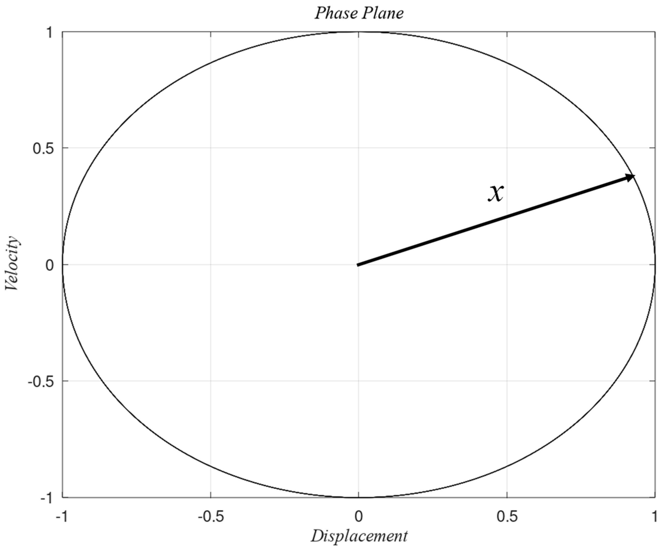
Figure 1 shows the evolution of the phase plane, and Figure 2 shows the phase plane of a Hamiltonian system with steady conditions.

2.2. Construction of the Phase Plane

The procedure for obtaining a phase plane with analytical models is straightforward because the state variables can be calculated by deriving the time series. In addition, the phase plane of a single frequency signal, such as an encephalogram signal, can be constructed with the original signal as one state variable, and the other state variable can be obtained by shifting the original signal by one-quarter of its period. Nevertheless, vibration data cannot be integrated numerically, and the phase plane cannot be constructed using the original signal and its shifted values [37].
The phase diagram from an accelerometer must be obtained by processing the time series to find the velocity and displacement components. Numerical integration introduces errors since it calculates the explicit integration instead of finding a function. Another characteristic of vibration signals is that they result from many frequencies and nonlinear components; therefore, they cannot be integrated only using the shifting principle. In addition, the spectrum domain integration is inadequate since the Fourier transform eliminates the nonlinear terms.
A new method is applied to overcome the difficulties of building the phase plane from the acceleration data. The method is based on two principles: decomposing the original data into a set of time series and integrating using the shifting principle. The original data are separated into discrete time series using the empirical model decomposition (EMD) method. The EMD decomposes the time series into a set of intrinsic mode functions (IMFs), and each IMF has a dominant frequency. The integration is conducted by shifting each IMF a quarter of its fundamental frequency; the integrated time series is built by recomposing the shifted signals and adding the shifted IMFs together. The advantage of the EMD over the Fourier decomposition is that every IMF keeps the transient and nonlinear components of the original signal. The original signal is fully reconstructed, whereas the Fourier decomposition cannot completely rebuild the original signal [38]. The acceleration signal is decomposed into a series of the following form:
a t = i = 1 n I M F i t + R n t
The decomposition produces n number of I M F , and R n are the residuals.

2.3. Recurrence Plot

The trajectory that the system describes in a phase plane can be represented as vector:
x ¯ = x ¯ 1 ,   x ¯ 2 ,   . , x ¯ n
where x ¯ i is the state variable vector that is obtained at every measurement. This vector is calculated at every cycle, as shown in Figure 2. The vector components are the position and time values at time i. From this vector, the recurrence plot is calculated as follows:
A i j = 1   :   x ¯ i = x ¯ j 0   :   x ¯ i x ¯ j     i , j = 1 , , N
where N is the number of data in the time-series vector. Since A i j is a matrix of ones and zeroes, it reflects the system’s dynamic. That is the reason for calling it the recurrence plot. Due to the time-series nature, it is impossible to have identical vectors; thus, the recurrence plot is calculated with a tolerance as follows:
A i j = 1   :   x ¯ i x ¯ j < ε , 0   :   x ¯ i x ¯ j > ε ,         i , j = 1 , , N
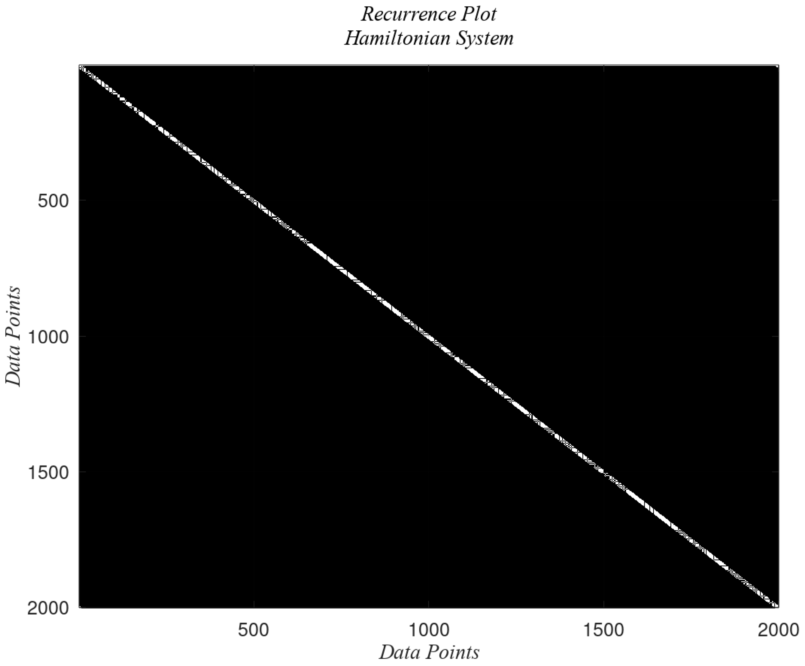
where ε is a tolerance value. The tolerance should be less than 10% of the mean diameter of the phase plane, or five times larger than the standard deviation of the observational noise. The recurrence plot of a Hamiltonian conservative system will be a single diagonal, as shown in Figure 3.
The white lines in Figure 3 are the one values of A i j ; the rest are zeroes. This simple example was calculated with 2000 data points that represent the fundamental period of a sine wave function. The horizontal distance between the diagonals is equivalent to the fundamental period of the system’s response. This example represents the ideal system; any variations of this plot are related to nonlinearities, transient responses, and the presence of multiple frequencies. As stated before, there are two procedures to evaluate the implications of these variations. The first evaluation is the quantitative analysis (recurrence quantitative analysis [21]). The analysis includes several parameters that measure the deviation from an ideal system. Table 1 lists the most commonly used parameters and describes them.
Table 2 includes the RQA parameters for a Hamiltonian system with a single diagonal. The parameters correspond to a time series of two thousand points. It is clear that the longest diagonal has the number of data points, the recurrence rate is the one over the number of points, and the determinism and entropy have the minimum values.

2.4. Topology Analysis

The recurrence plots’ topology represents deviations from the ideal Hamiltonian conservative system. The topology analysis determines the possible causes of these variations. The most common patterns are as follows:
The recurrence plots have different topologies, representing the state variables and helping to describe the dynamic behavior of the mechanical system. Some of the most characteristic pattern meanings include the following:
-
Stationary systems show homogenous patterns (continuous diagonals);
-
Slow state changes display horizontal and vertical lines;
-
Non-stationary systems display drifts;
-
Constant variations of the states show single points;
-
Sudden changes in the system show clusters of white points;
-
Drifting systems produce black fringes.
In general, the diagonal lines are the principal characteristic because they represent the return of the trajectory along the phase to the initial point or the same point at its first period. Only diagonal lines define the pattern for a periodic system. The diagonal length is related to the amount of time the trajectory takes. A short and irregular length represents a chaotic system. Tilted diagonals are characteristic of recurrent states at different intervals. The irregular separation between diagonals comes from irrational frequency ratios.

3. Field Measurements

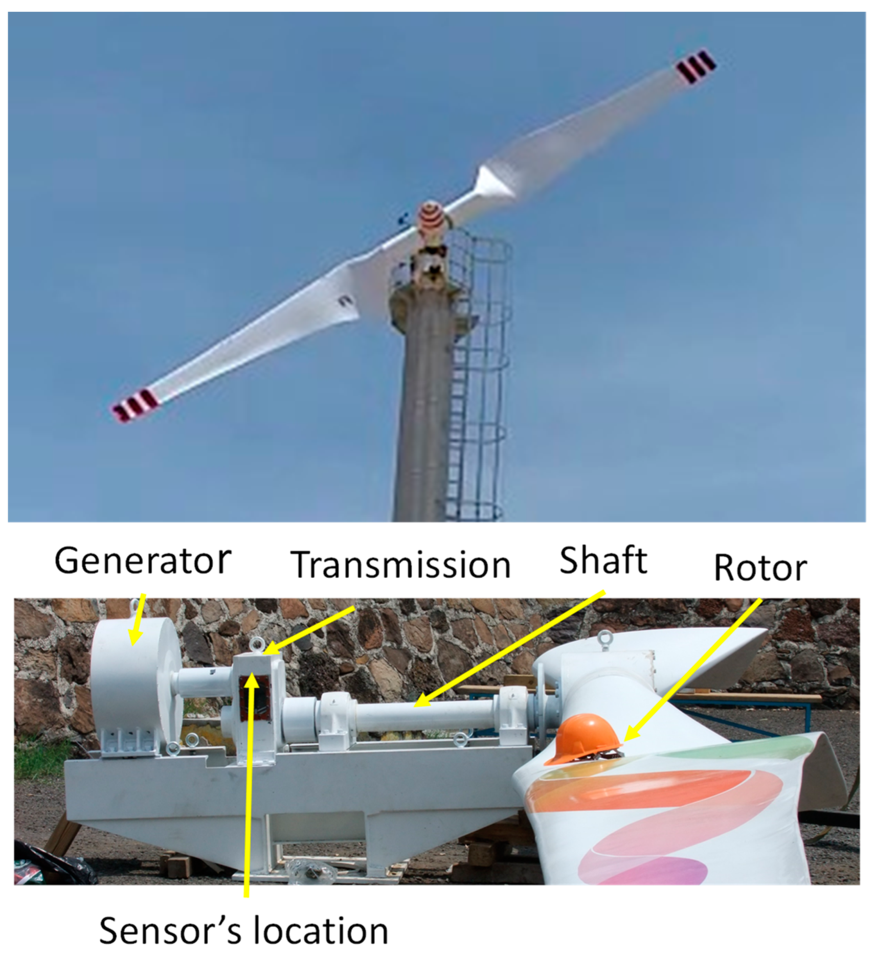
The data were recorded at an experimental wind turbine located at the Autonomous University of Queretaro. The wind turbine consists of a 12 m two-blade rotor connected through a main shaft, which moves a 1:2 gearbox increaser, which rotates a 12 KW permanent magnet electric generator. Figure 4 shows a picture of the experimental wind turbine.
The wind turbine is mounted on an 18 m tower. The gearbox was instrumented with a three-axis accelerometer and three Hall-effect magnetometers connected orthogonally. The field data were recorded on different days. Some measurements were recorded at low wind speed and without the rotor’s rotation; other data were recorded when the rotor was rotating.
The measuring system consists of the following:
-
A three-axial MEMs magnetometer with a resolution of 0.58 mgaus/LSB (least significant bit) and a range of ±16 gauss;
-
A three-axial MEMs accelerometer with a resolution of 0.244 mg/LSB with a range of ±8 g;
-
An FPGA data processor;
-
A data acquisition system with a sampling rate of 1 kHz.
This paper includes only the data recorded on four different dates. Table 3 shows the four cases.
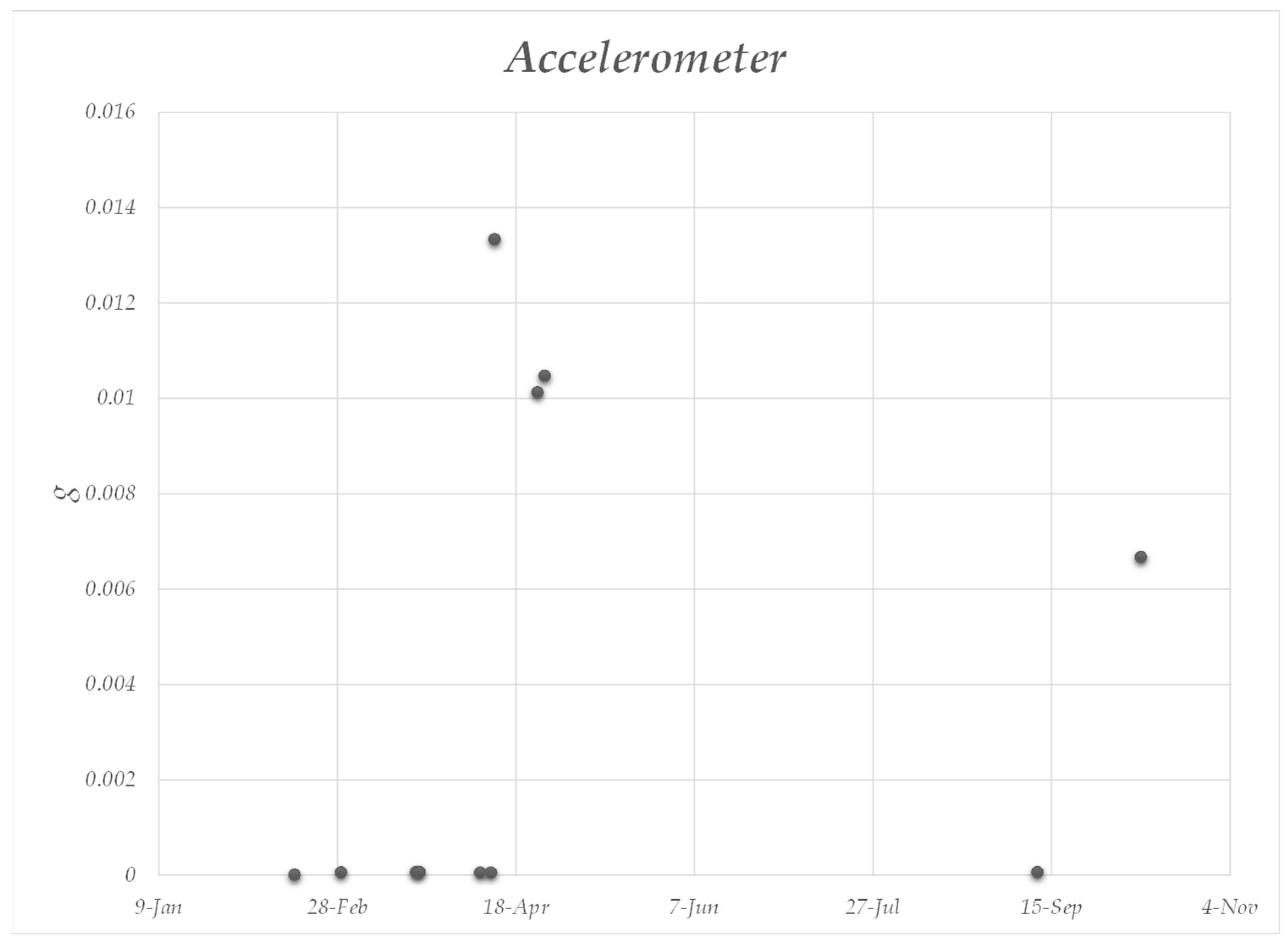
The frequency spectrum of all the measurements was calculated to complement the analysis, and the highest peaks were recorded. Figure 5 and Figure 6 compare the accelerometer and magnetometer data.
The four data points were selected from the higher amplitude values. The following section describes the results of the recurrence plots of both signals, the accelerometer measurements, and the magnetometer data.

4. Results

This section is divided into two parts: the analysis of the accelerometer data and the magnetometer data, respectively. For each analysis, four cases are included in this paper. Case 0 corresponds to measurements when the rotor did not rotate. The vibration measurements correspond to the tower movements due to the low-speed wind velocity, and the magnetometer measurements correspond to the magnetic field of the permanent magnets. Due to the generator construction, the permanent magnets are the rotating element, and the solenoids are the stator.
Before analyzing the data with the recurrence plot, the measurements were analyzed using the Fourier spectrum and the wavelet transform. These analyses are used as a reference to determine the dynamic conditions. The wavelet transform was the basis for producing the spectrograms, also known as time–frequency maps. The best technique for vibration signals is the continuous wavelet transform with the Morlet mother function. The parameters used in the further analysis were determined using the frequency range of the dominant peaks.

4.1. Analysis of the Accelerometer Data

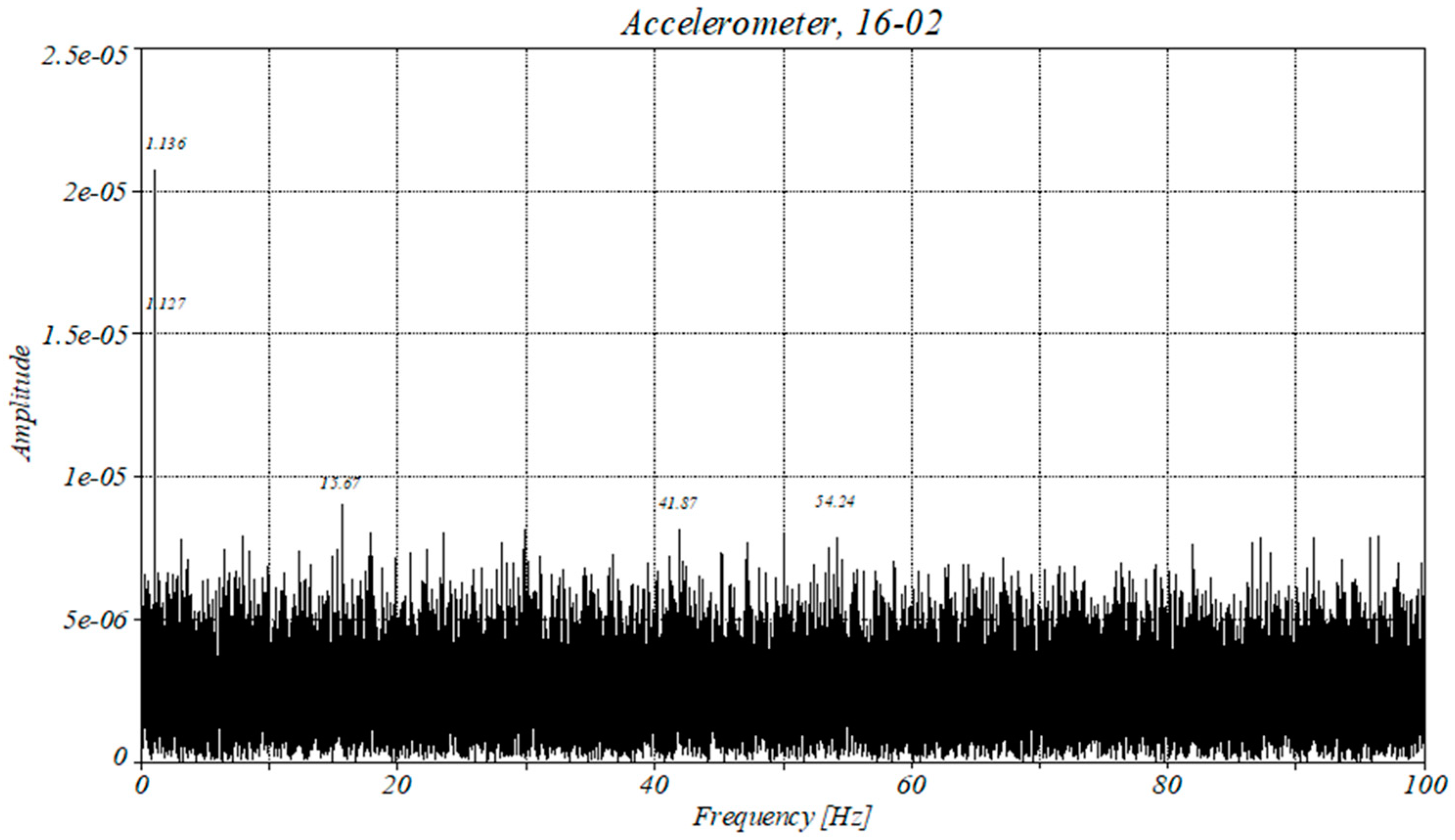
Figure 7 shows the frequency spectrum of the accelerometer data corresponding to case 0. The spectrum shows that the amplitude is relatively low, and the dominant peak corresponds to the tower movement due to the wind pressure. The rest of the peaks have not been identified as having any vibration source.
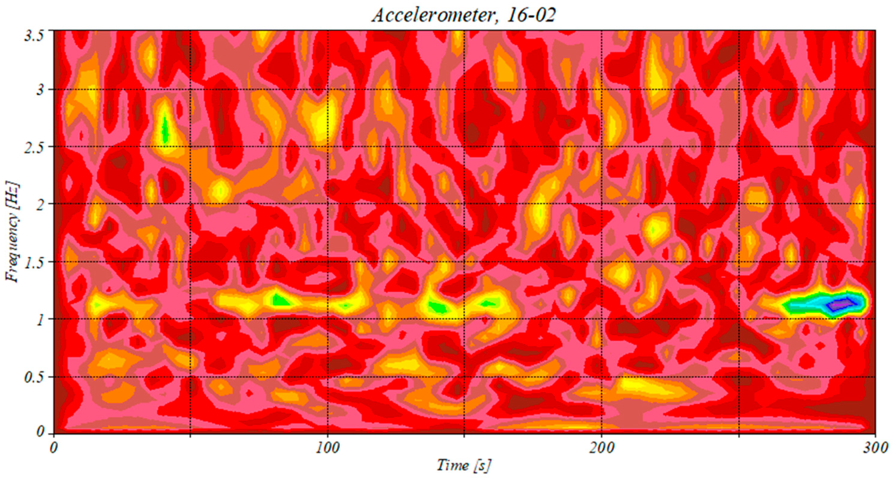
The spectrogram confirms a single dominant frequency corresponding to the tower’s movement (Figure 8).
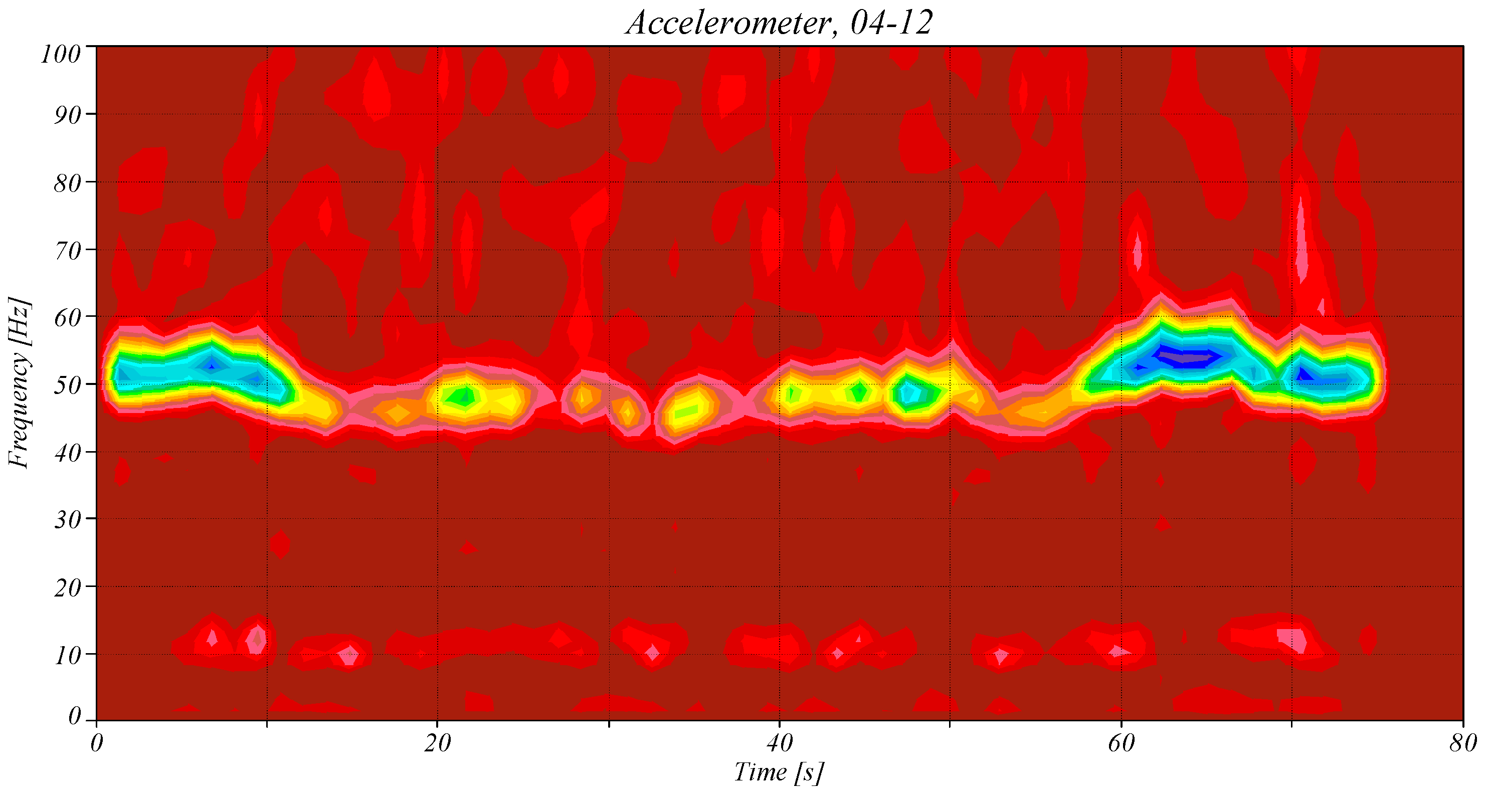
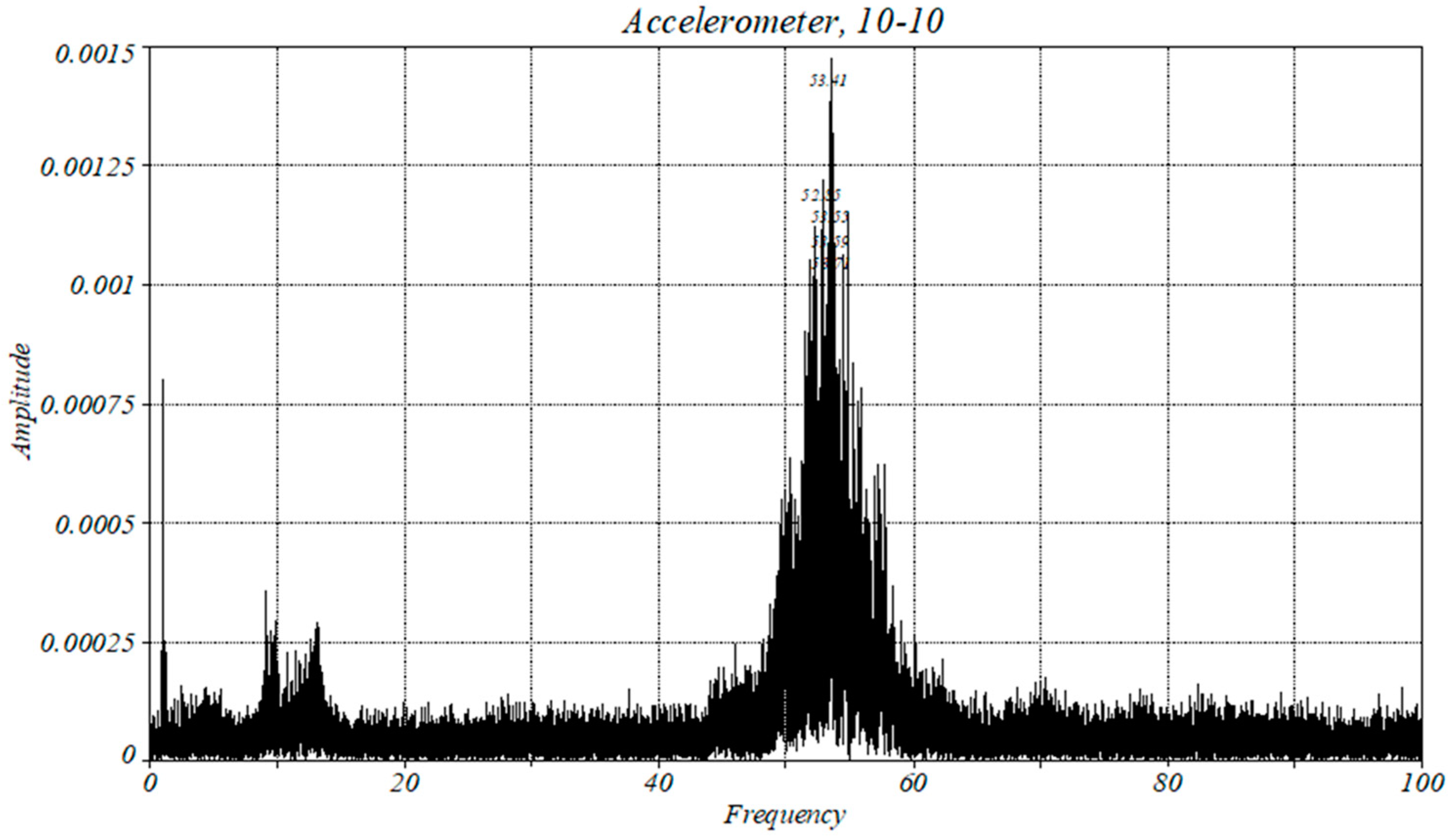
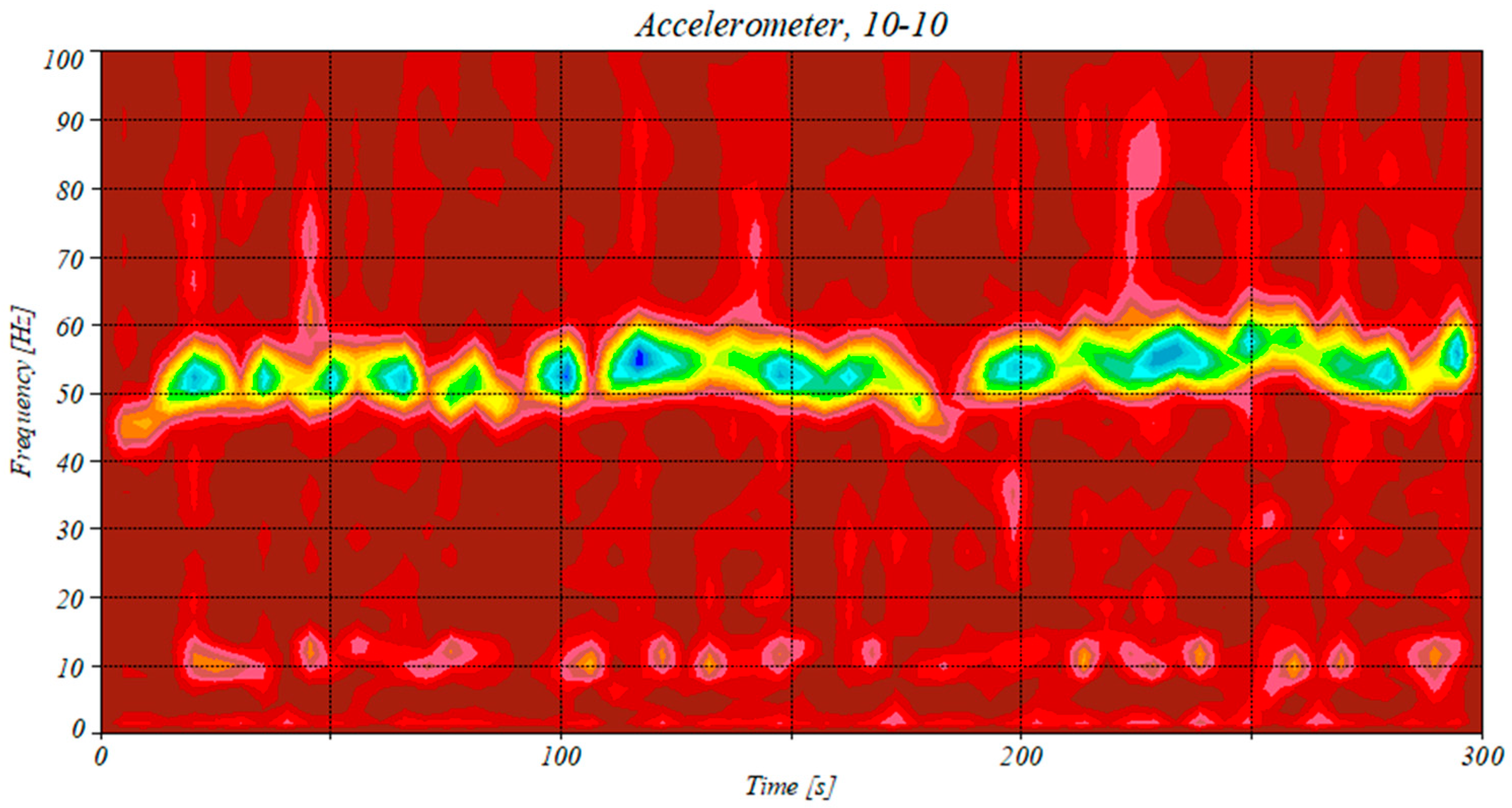
Figure 9 shows the frequency spectrum of case 1. In this case, the dominant frequency corresponds to the gear-mesh frequency, the second-highest peak corresponds to a bearing frequency, and the peak around 1.07 Hz is the generator’s rotating speed. The wind speed variations are identified in the spectrogram as discontinuities and changes in frequency (Figure 10). The dominant peak occurs at 51 Hz, which corresponds to the gear-mesh frequency (the input gear has 47 teeth, which when multiplied by the rotating frequency gives the gear-mesh frequency, and the spectrum shows lateral side bands with a separation of the rotating speed, which is a characteristic pattern of the gear-mesh frequency). The gearbox roller bearings produce the other peaks.
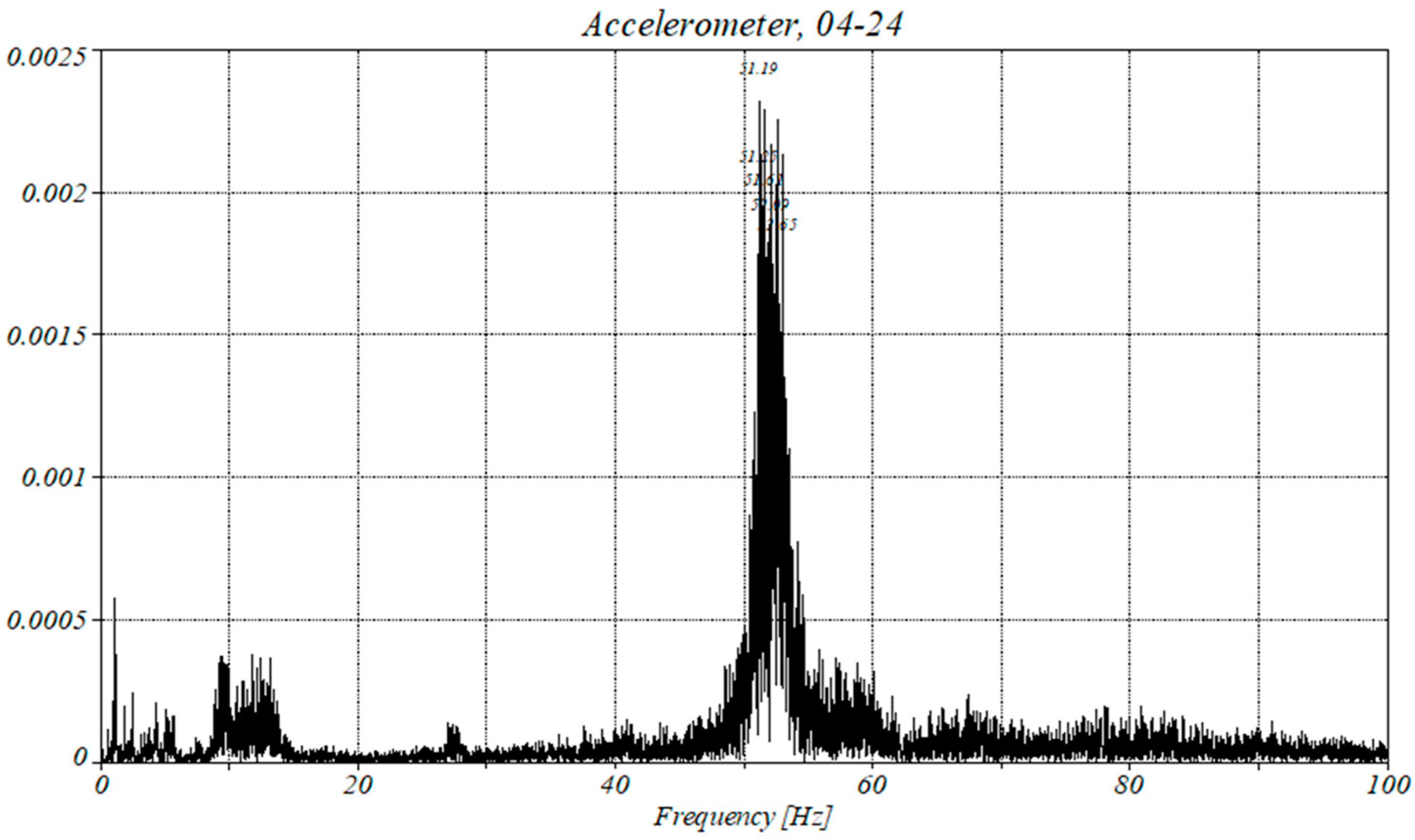
Figure 11 and Figure 12 show similar results as described in the previous paragraph. The frequency spectrum and spectrogram correspond to case 2. These figures confirm the vibration pattern of the wind turbine under high wind speeds. Figure 13 and Figure 14 show case 3’s frequency spectrum and spectrogram. The only difference from the other two cases is the amplitude. The dominant frequency has values similar to those of cases 1 and 2.
Table 4 summarizes the values of the highest amplitudes. When the generator is idle, the amplitude is relatively low; the other three cases have variations of 40%. The analysis of these variations corresponds to the conditioning monitoring system.
After the Fourier and the wavelet transform (spectrogram) analyses, the acceleration data were analyzed using the recurrence plot method described in the previous sections.

4.2. Application of the RPs to the Accelerometer Data

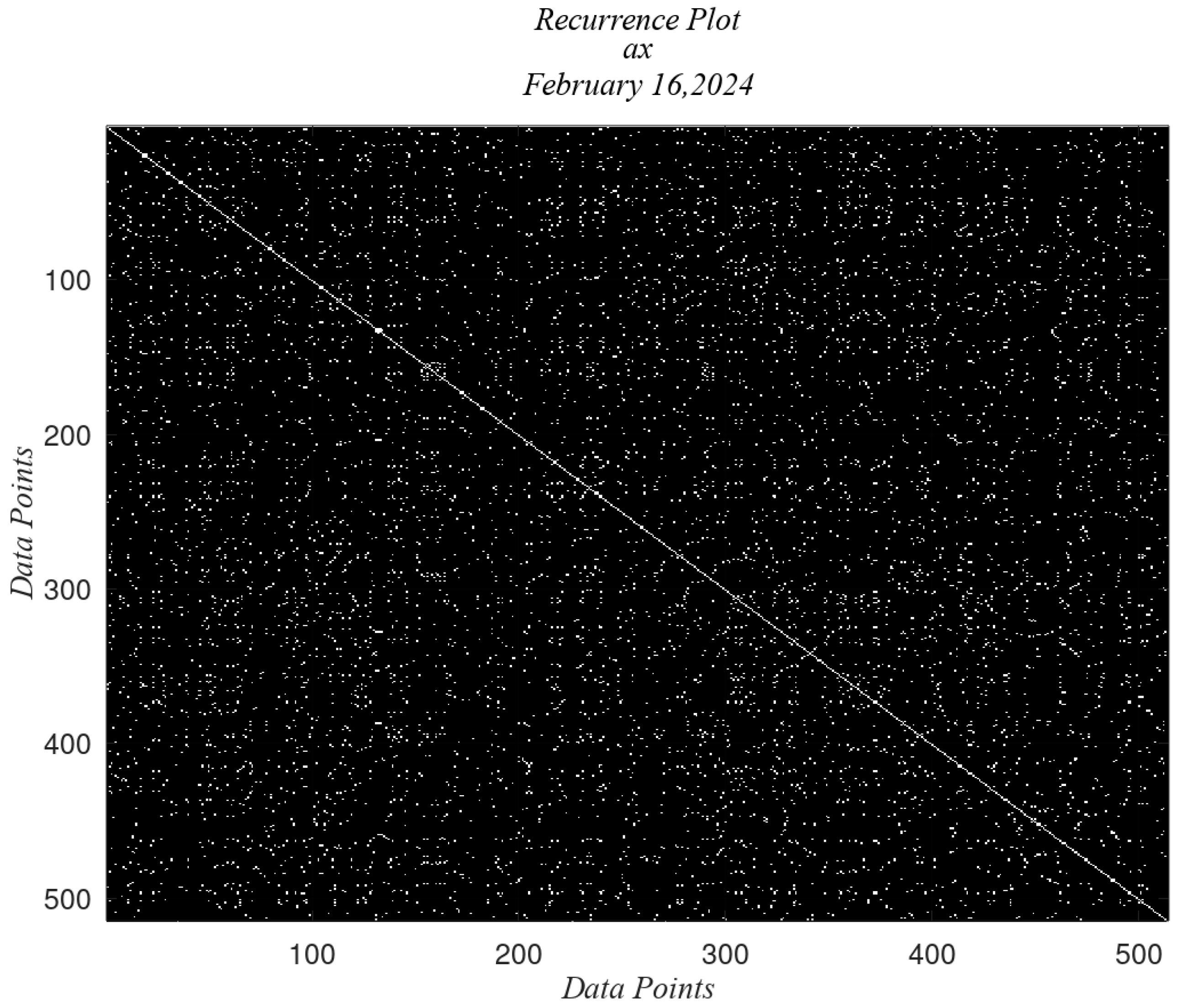
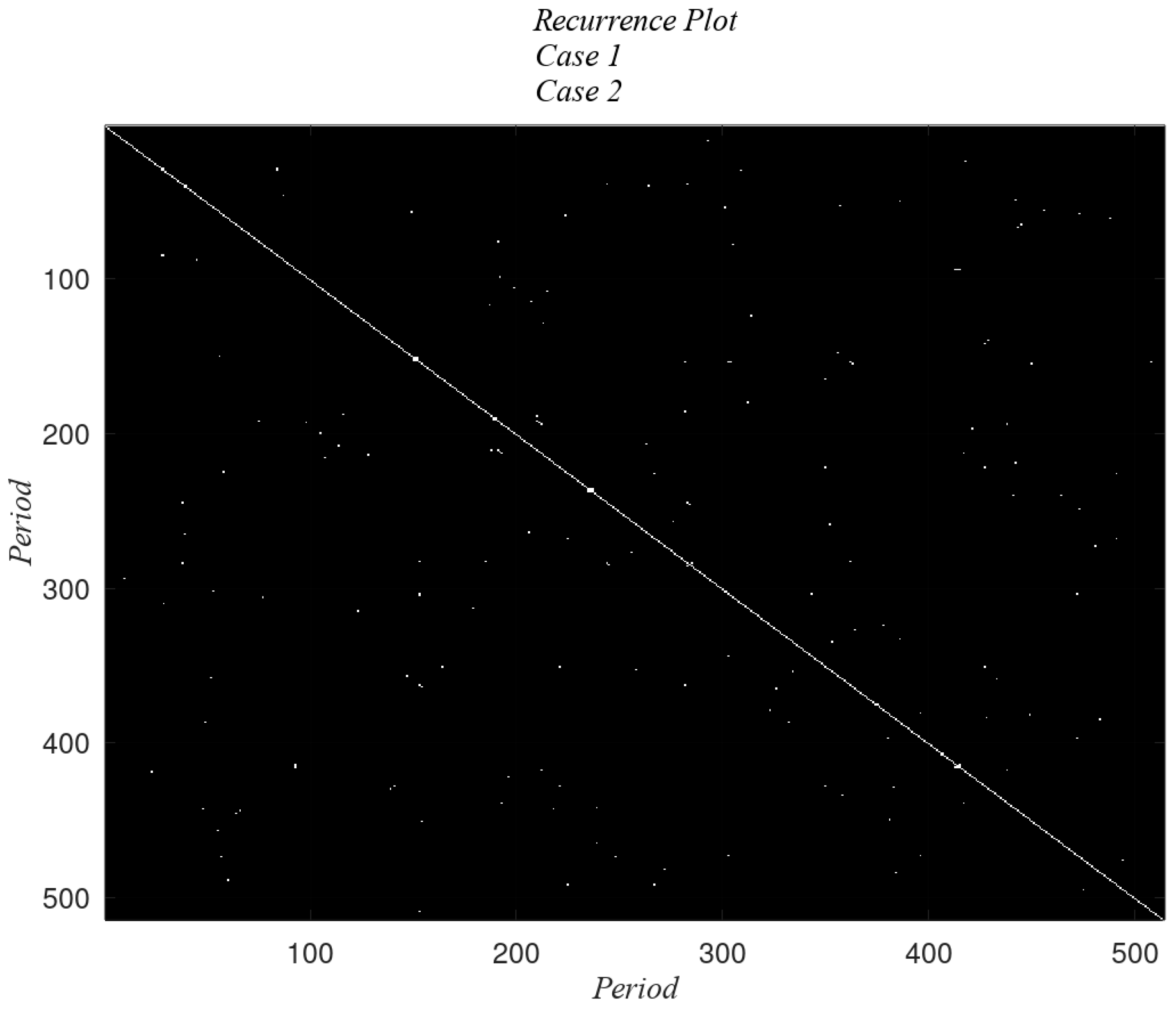
The acceleration data have dominant peaks at frequencies around 50 Hz; thus, the periods correspond to 20 data points. Figure 15 shows the RP of the no-wind condition. This figure shows only a dominant diagonal; the remaining points are randomly distributed throughout the image. The graphs were limited to 500 data points. The number of points is determined from the frequency of the highest peak and the sampling rate of 1000 Hz. Besides the main diagonal, the figure shows distributed points without a defined pattern, clustering, or horizontal and vertical lines. This plot is the reference since it is considered the unload condition. The number of points was selected to display the lowest frequency and the 50 Hz loops.
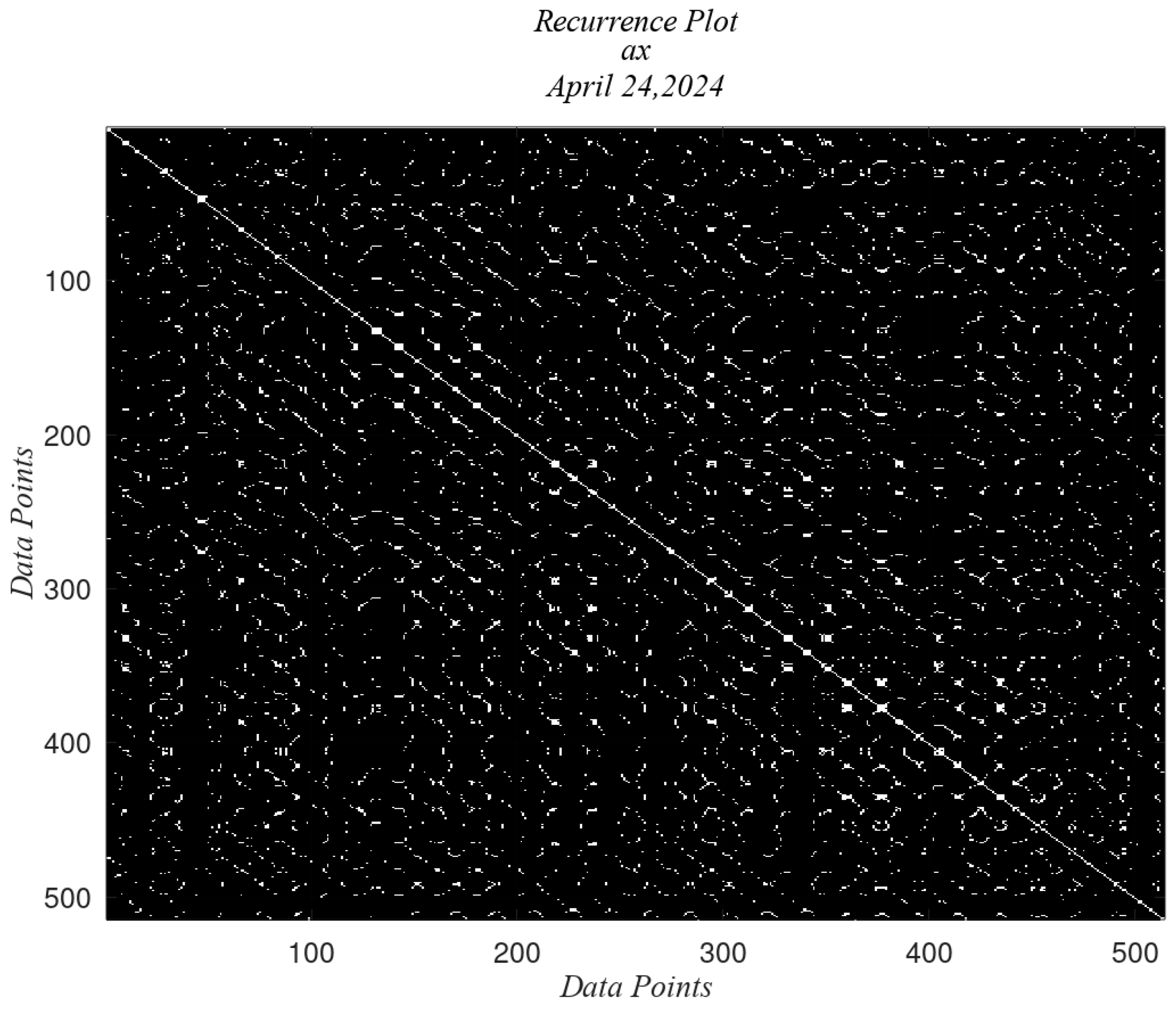
Figure 16 shows a different pattern. Although the diagonals are discontinuous (except the main diagonal), several diagonals are clearly separated around 20 points. The figure also shows clusters and vertical and horizontal lines (these lines are discontinuous, but it is easy to identify the hollow areas).
The lateral diagonals are discontinuous because some of the loops coincide outside the tolerance. Those that lie within the tolerance range appear as white dots with a trend and, ideally, a straight line. This figure shows 25 lateral diagonals separated by 20 data points, forming the 500 data points of the recorded data.
Figure 17 shows the recurrence plot of case 2. In comparison with case 1, this figure shows longer diagonals and fewer clusters. In addition, the horizontal and vertical diagonals are more difficult to identify.
Figure 18 shows the recurrence plot for case 3. In this case, the diagonals are less defined, and the clusters are similar to those in case 1.
The following section describes the results obtained with the magnetometer data. All the figures are equivalent to the accelerometer data and are presented in the same order.

4.3. Analysis of the Magnetometer Data

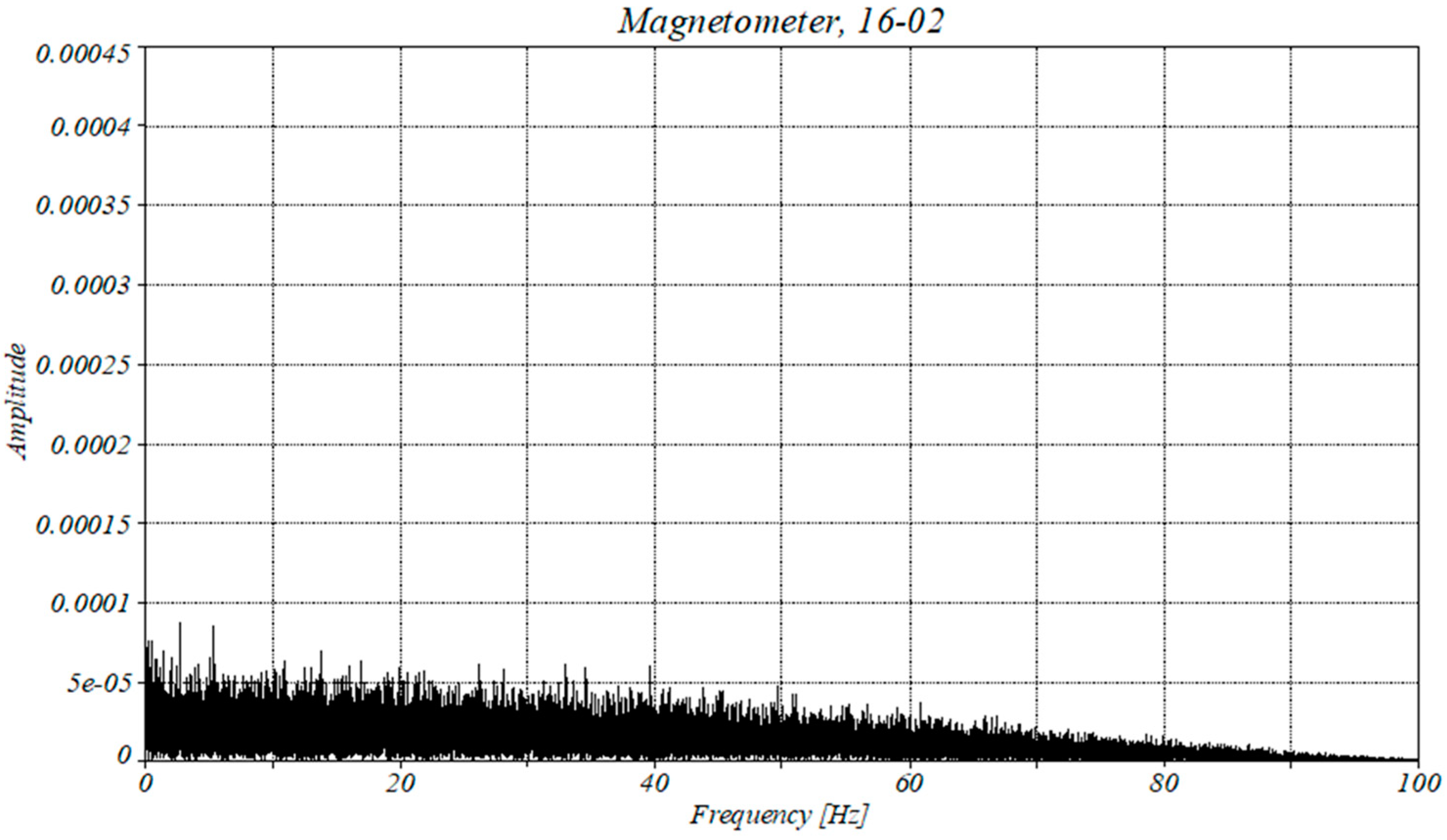
Figure 19 shows the frequency spectrum obtained with the magnetometer data without rotation (case 0). Only a very low-frequency component is related to the permanent magnet field.
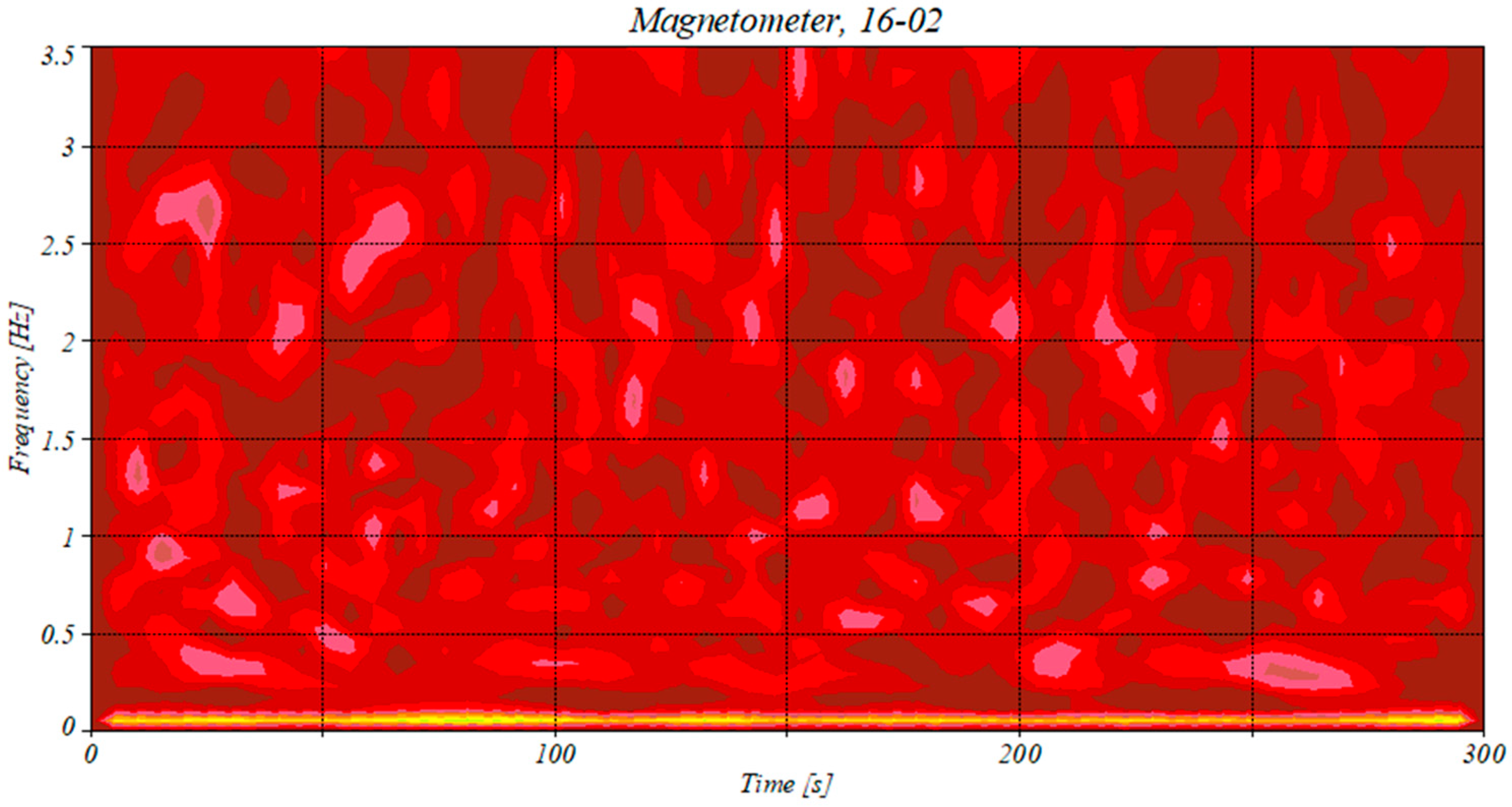
The spectrogram (Figure 20) shows the low-frequency component and a noisy response elsewhere.
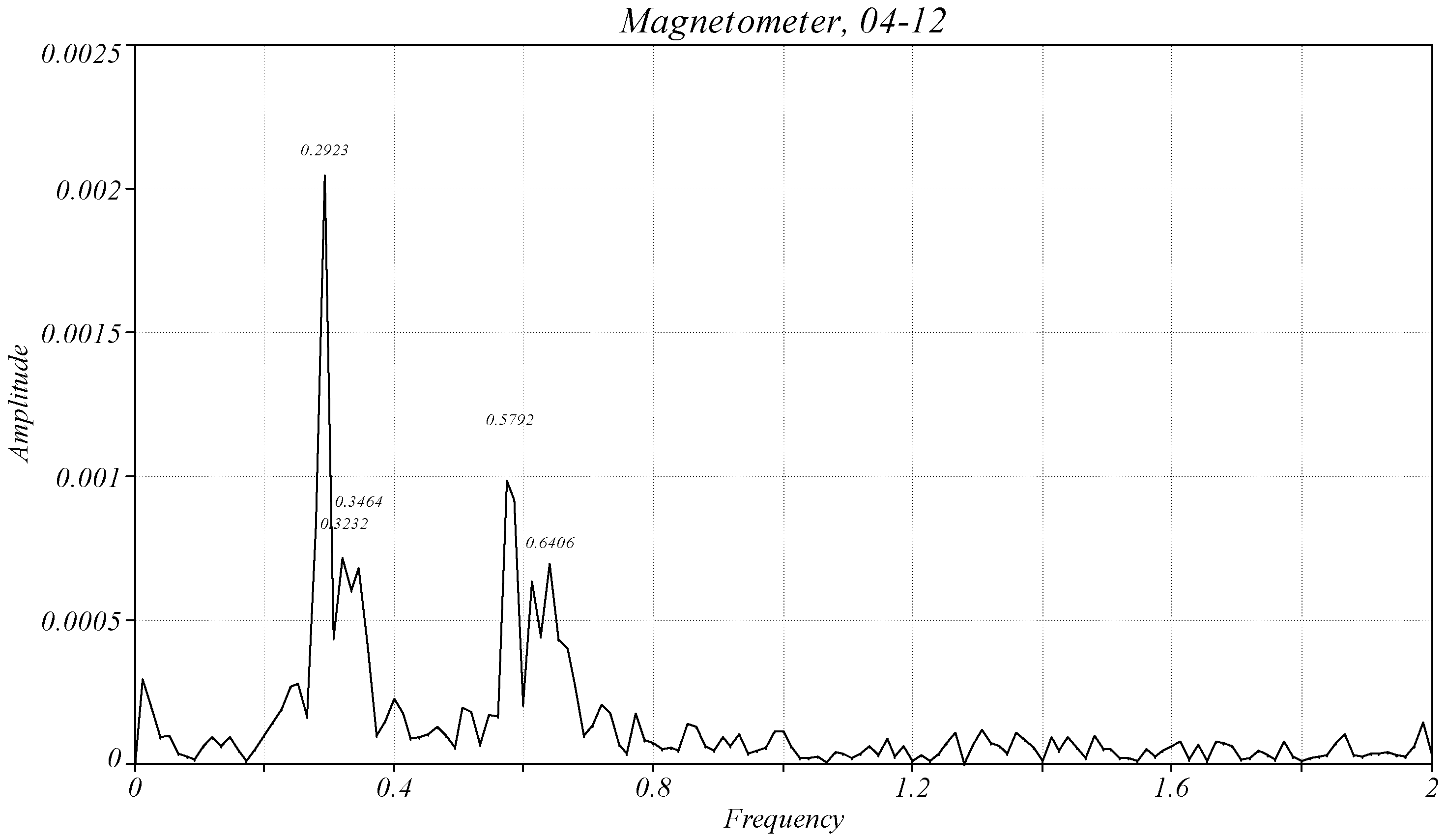
Once the generator starts rotating, the dynamic response is entirely different. Figure 21 shows the frequency spectrum. It shows two dominant peaks at 0.29 Hz and 0.58 Hz. These frequencies appear in all the spectra when the generator rotates. They are associated with magnetic low-frequency variations. The dominant frequency is 0.29 Hz, and it has a harmonic at 0.58 Hz. The other two have asynchronous modes.
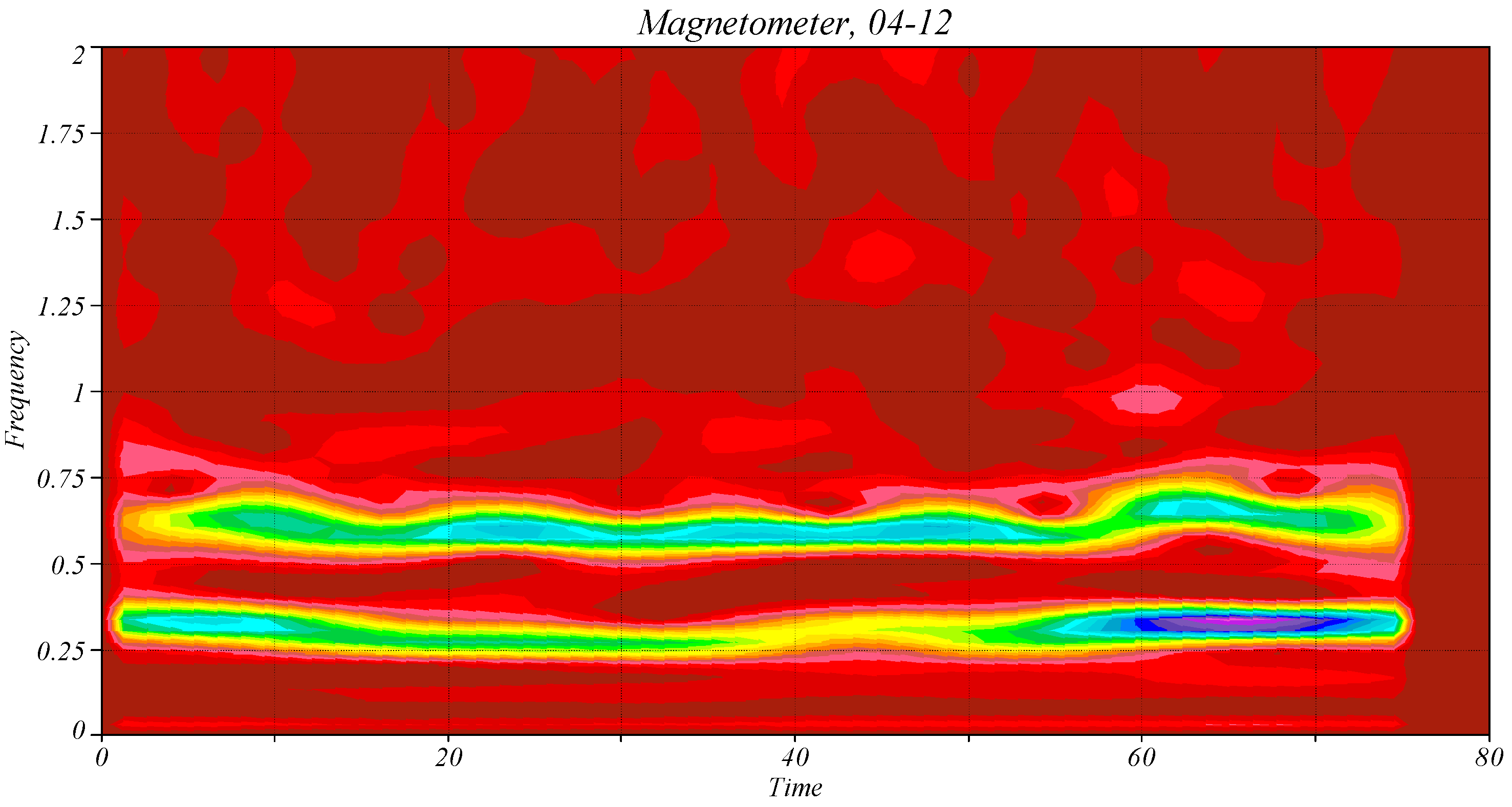
The spectrogram (Figure 22) shows the same dominant frequencies, which remain constant at all times.
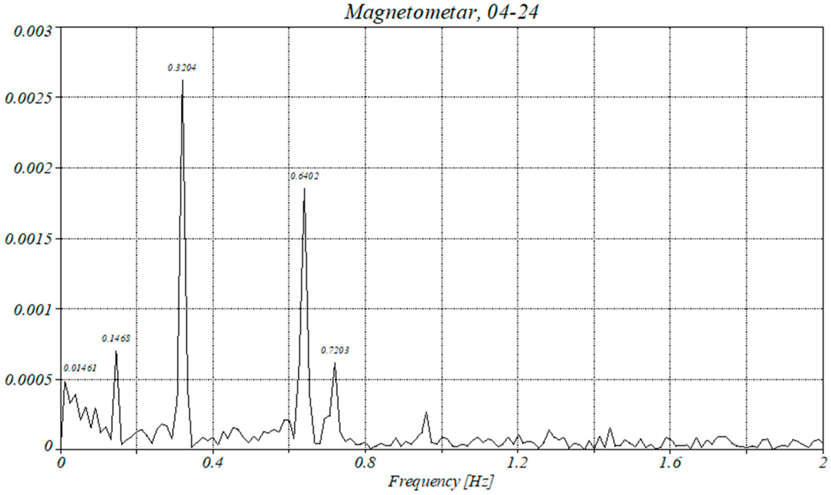
Case 2 shows a similar pattern to case 1. The frequencies vary because of the wind speed but are in the same range (Figure 23). It has two extra peaks, at 0.14 Hz and 0.72 Hz. The spectrogram (Figure 24) shows slight time variations.
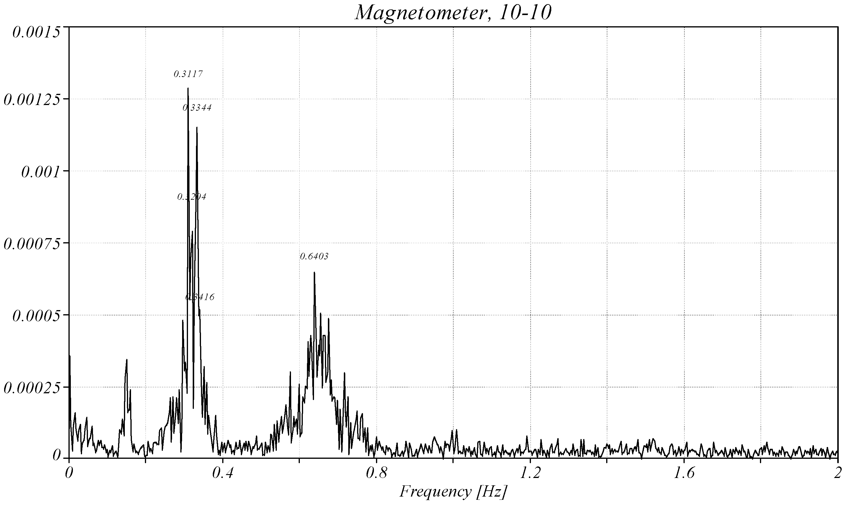
Case 3 behaves the same as case 1; the only difference is a small amplitude variation. Figure 25 shows the frequency spectrum, and Figure 26 shows the spectrogram. The wider variations in the spectrogram reflect wind speed variations.
Table 5 summarizes the highest amplitude values. The amplitude variations follow a similar pattern to the acceleration data, but the relative variations differ. Particularly, when the rotor is idle, the permanent magnet field shows a very low-frequency oscillation.

4.4. Application of the RPs to the Magnetometer Data

The recurrence plots complement traditional vibration analysis and provide a means for understanding the non-stationary and nonlinearity responses. Since the magnetometer is more sensitive at low frequencies, it was necessary to analyze a large number of points. The lower frequencies require a larger number of points. In the case of the magnetometer, the number of points for producing the RPs was 8000 data points since it covers loops of the lowest frequency (0.25 Hz).
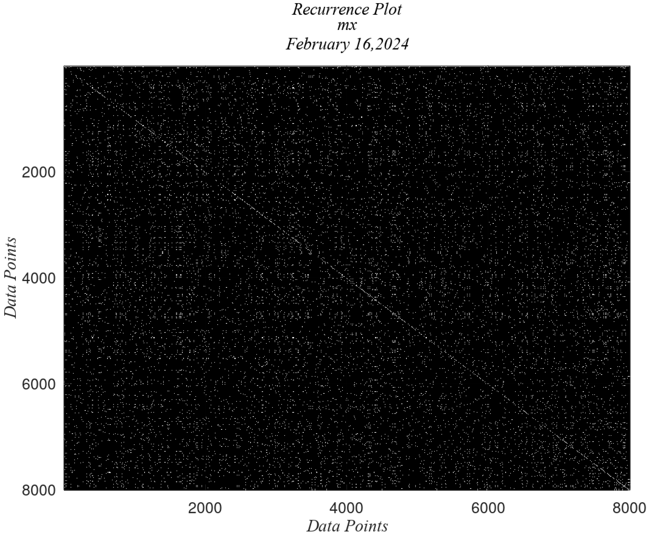
Figure 27 shows the RP when the rotor is idle (no rotation). Besides the main diagonal, the graph shows a heterogeneous distribution of points without clusters or dominant lines.
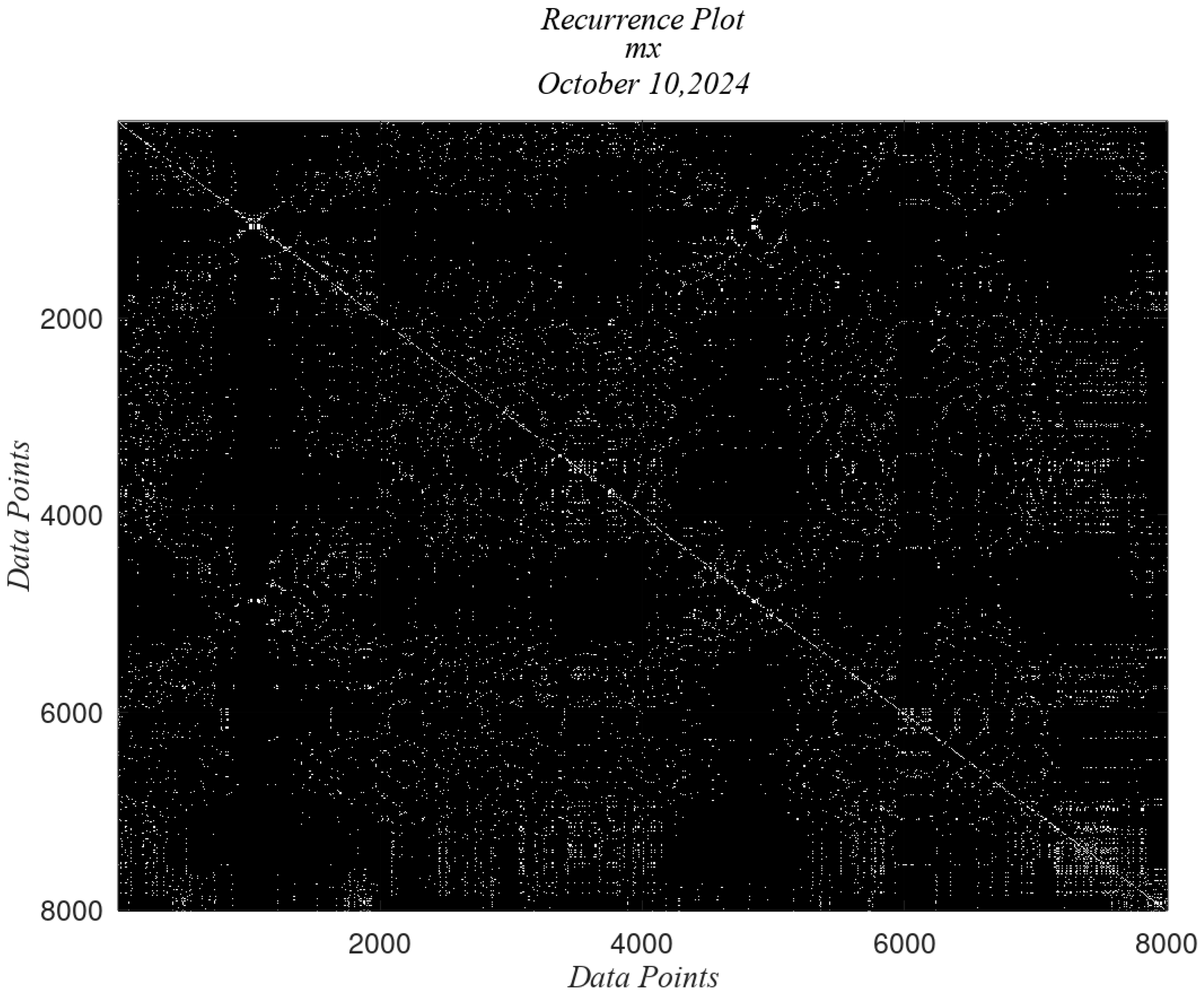
Figure 28 shows case 1 results. This graph has well-defined clusters and horizontal and vertical patterns reflecting nonlinear responses. These patterns are associated with nonlinear magnetic field variations that are difficult to identify in the frequency spectrum or the spectrogram. The following section describes the analysis of the quantitative analysis. The RP for cases 2 and 3 are shown in Figure 29 and Figure 30.

5. Discussion

The topology analysis of both recurrence plots, namely the acceleration and magnetometer data, identifies the sources of deviations from the ideal Hamiltonian system. For the four cases, both data sources show diagonal discontinuities, clusters of values, vertical and horizontal non-continuous lines, and black fringes. The diagonal discontinuities are due to non-stationary behavior, sudden energy changes, and external perturbations. The evident source of perturbation is the wind speed and the nonlinear responses. Other evidence of sudden changes is the presence of white clusters, while the black fringes are due to slow deviations from the steady state condition.
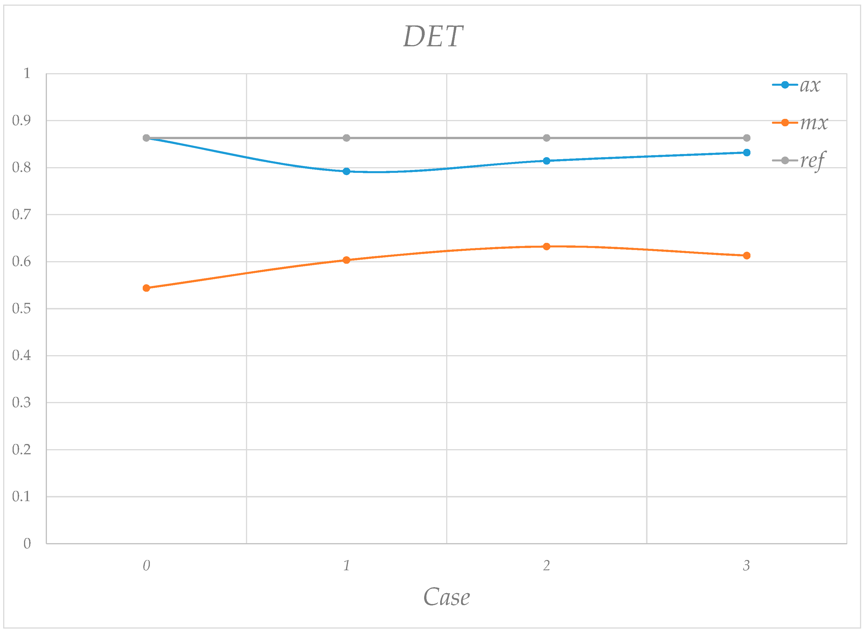
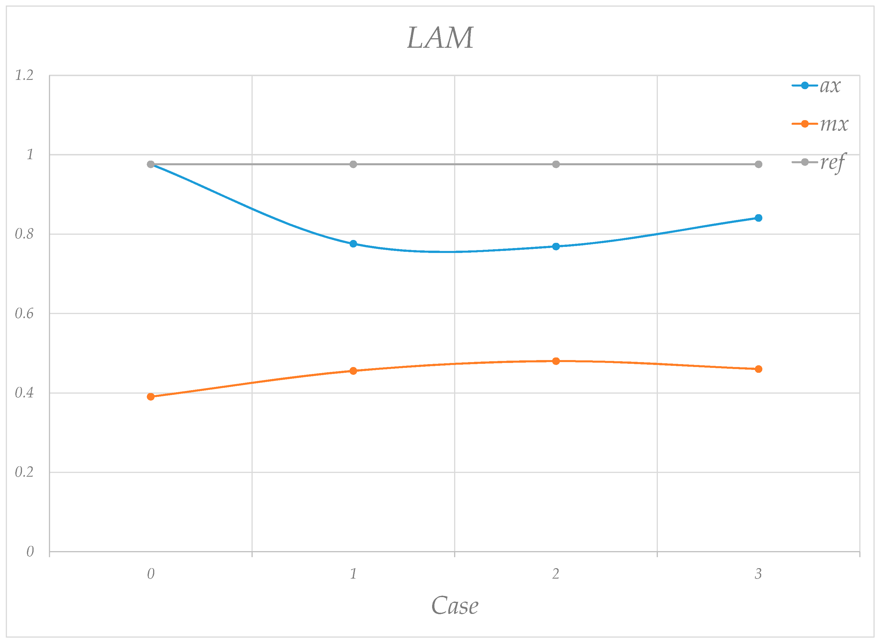
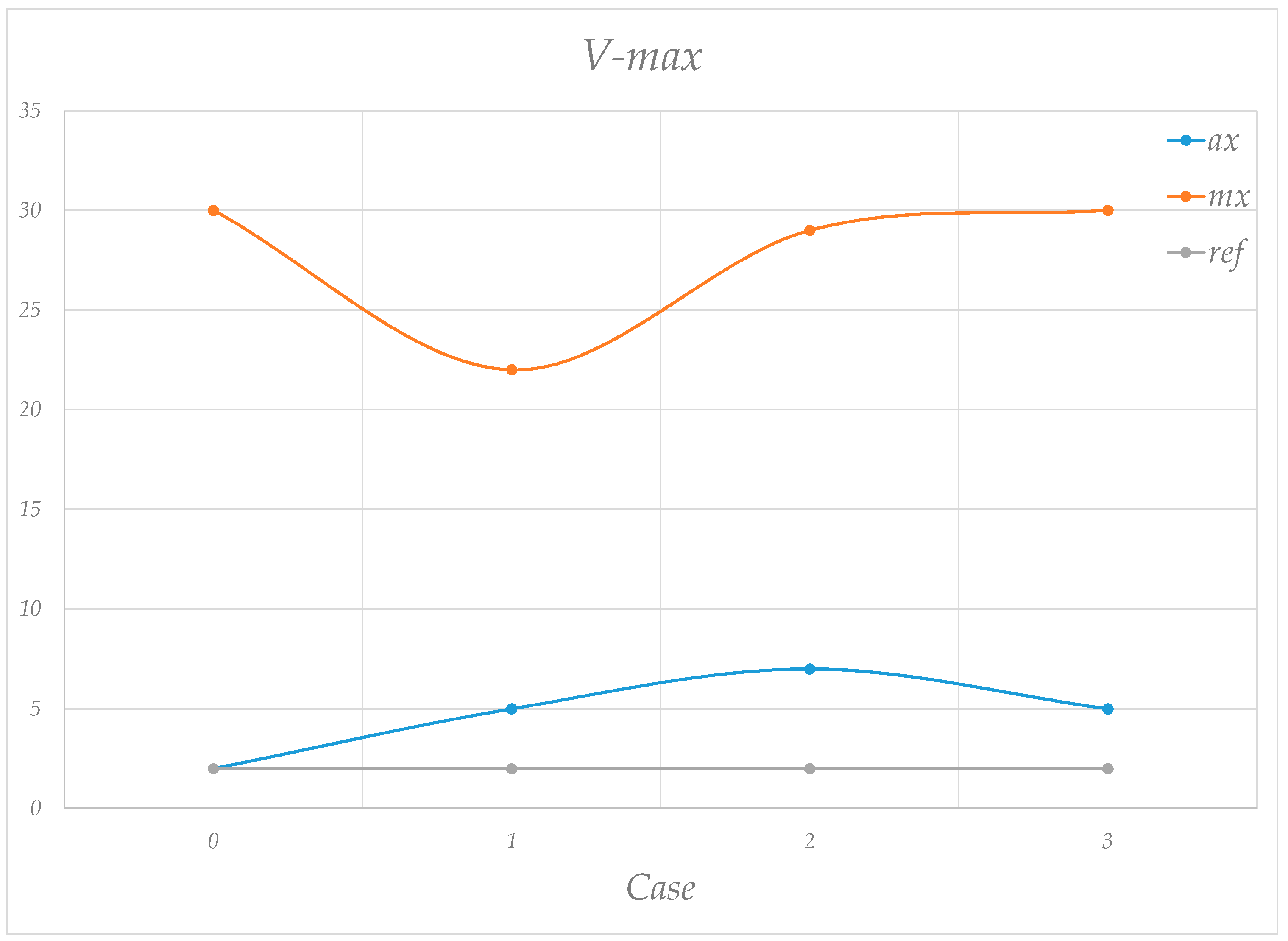
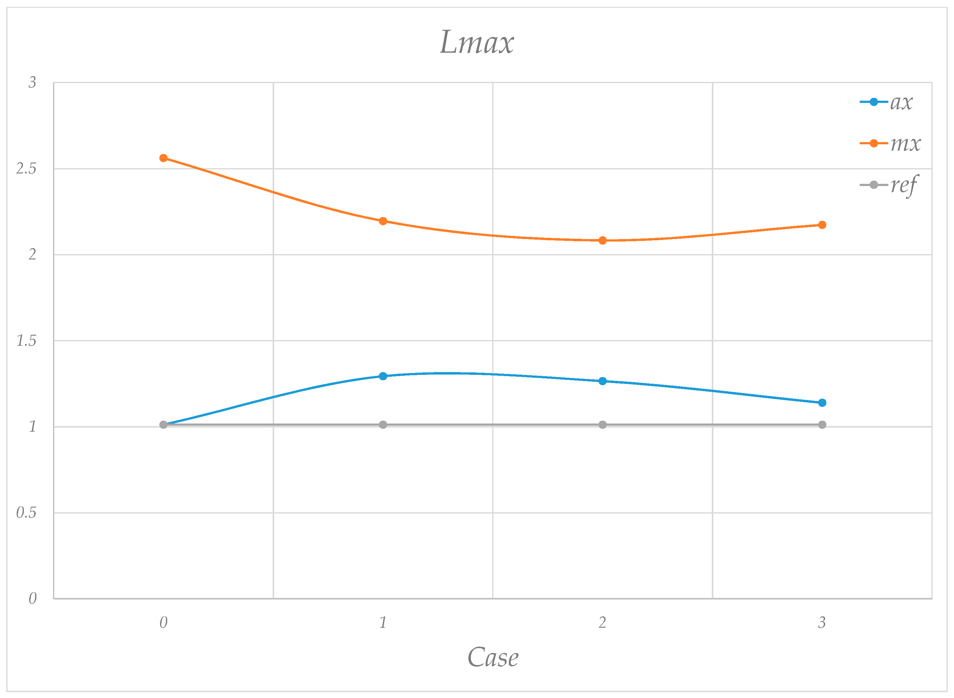
The following figures show the analysis of RQA. The graphs include the values for the accelerometer and the magnetometer, with reference to the no-wind condition (case 0). The values correspond to the four cases.
Figure 31 compares the recurrence rate for the accelerometer and magnetometer data. The accelerometer data show the highest value in case 1, whereas the magnetometer data show the largest value in case 3.
Figure 32 shows the determinism. This parameter measures the percentage of points that lie on the diagonal. It is less sensitive to the acceleration data than the magnetometer data. Thus, the analysis of the magnetometer data with this parameter better reflect the nonlinear behavior.
Figure 33 shows the laminarity parameter. In this case, the acceleration data better reflect the non-linear behavior. The acceleration data show an inverse behavior to the magnetometer data, and the magnetometer data have a similar pattern to the maximum signal amplitude.
Figure 34 shows the longest vertical line. This parameter’s pattern is similar to RR’s, which suggests that sudden changes are less sensitive to acceleration data. The longest diagonal is plotted in Figure 35.
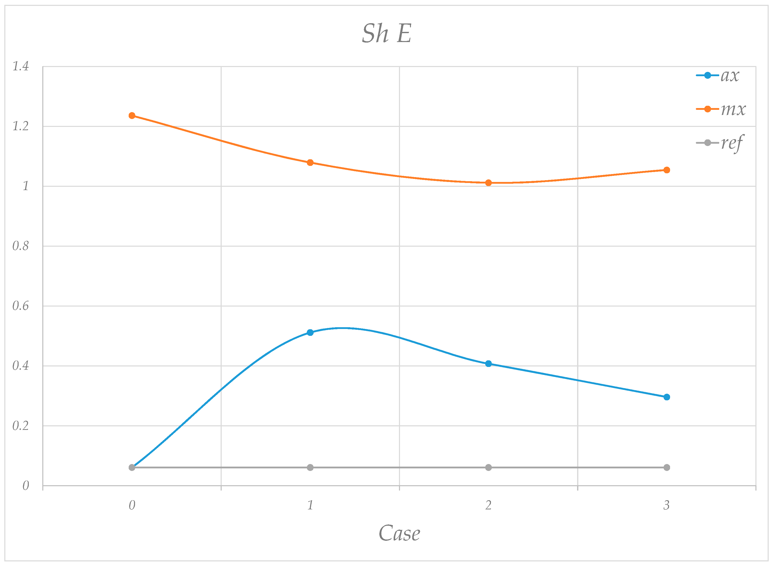
The last analysis is the Shannon entropy (Figure 36). The variations in the magnetometer data have a higher impact on the Shannon entropy than the acceleration data.
The cross-recurrence plot (CRP) was also applied to identify the difference between the two measurements [24]. The CRP identifies the coincidences between two RPs. In this case, the analysis was applied to cases 1 and 2. Figure 37 shows the CRP of the accelerometer data, and Figure 38 shows the magnetometer data.
Both figures show that the recurrence plots hardly coincide, and the wind turbine’s dynamic behavior has significant variation. The comparison of Figure 37 and Figure 38 with the recurrence plots shows few coincidences besides the diagonal. To monitor the dynamic behavior, all the parameters and the CRP provide a powerful tool for monitoring sudden changes, and, if these changes are not related to operating conditions, then they are a reasonable estimation of premature failures.
Regarding the authors’ knowledge, other analysis techniques, such as cyclostationarity or spectral kurtosis, are helpful for different problem detection. Cyclostationarity provides better results for signals with periodic statistical variations; spectral kurtosis detects impulsive events but might not detect complex nonlinearities. Recurrence plots are the most robust tool for identifying nonlinear dynamics and chaotic behavior.

6. Conclusions

Recurrence plots are an alternative tool for identifying nonlinearities in mechanical systems. This paper presents the application of the RPs to two different signals obtained in an Eolic generator. The data were generated with an accelerometer and a magnetometer. The accelerometer data were used as a reference to compare the effectiveness of using magnetometers as a data source for monitoring the operating conditions.
The accelerometer data show a good sensitivity to high frequencies, whereas the magnetometer has a good resolution at low frequencies. The recurrence plot analysis of both sets of data was able to identify the nonlinear and non-stationary behavior of the system. The analysis included the topology and the recurrence quantitative analysis. The quantitative analysis demonstrated that the magnetometer data provide better information regarding the system’s energy variations because it is more sensitive to changes in the operating conditions. Thus, the magnetometer can serve as an alternative sensor for monitoring sudden variations in operating conditions. This alternative method for monitoring a wind turbine overcomes the limitations of determining the operating conditions when measuring the wind velocity. The wind measurements have larger time intervals, whereas the magnetometer measures at higher sample rates; thus, monitoring with the magnetometer can identify gusty wind conditions and sudden variations that cannot be identified with the wind sensors. The analysis with the recurrence plots helps us identify the opportunity to monitor the wind turbine with a more sensitive method.
Recurrence plots are better when dealing with nonlinear or non-stationary signals. Cyclostationarity is best suited for signals with periodic statistical variations. Spectral kurtosis is recommended for detecting impulsive events but may not capture complex nonlinearities.
Future work involves the electronic implementation of an automatic system that continuously provides the RQA parameters for both signals.

Author Contributions

Methodology, L.M.-V.; Writing—original draft, J.C.J.-C. All authors have read and agreed to the published version of the manuscript.

Funding

This research received no external funding.

Data Availability Statement

The data presented in this study are available on request from the corresponding author.

Acknowledgments

The authors would like to thank CONAHCyT for supporting this work “Proyecto apoyado por el Conahcyt en el año 2023, Ciencia de Frontera con el número CF-2023-I-204”.

Conflicts of Interest

The authors declare no conflicts of interest.

References

  1. Jauregui-Correa, J.C.; Lozano-Guzmán, A. Mechanical Vibrations and Condition Monitoring, 1st ed.; Elsevier Inc.: Amsterdam, The Netherlands, 2020; ISBN 978-0-12-819796-7. [Google Scholar]
  2. Eckmann, J.; Oliffson, S.; Ruelle, D. Recurrence Plots of Dynamical Systems. Eur. Lett. 1987, 4, 973–977. [Google Scholar] [CrossRef]
  3. Webber, C.L.; Ioana, C.; Marwan, N.; Symposium, I.; Plots, R. Recurrence Plots and Their Quantifications: Expanding Horizons; Springer: Berlin/Heidelberg, Germany, 2015; ISBN 9783319299211. [Google Scholar]
  4. Marwan, N.; Webber, C.L. Mathematical and Computational Foundations of Recurrence Quantifications. In Recurrence Quantification Analysis; Marwan, N., Webber, C.L., Eds.; Springer International Publishing: Cham, Switzerland, 2015; pp. 3–43. ISBN 9783319071558. [Google Scholar]
  5. Thiel, M.; Romano, M.; Kurths, J. Spurious Structures in Recurrence Plots Induced by Embedding. Nonlinear Dyn. 2006, 44, 299–305. [Google Scholar] [CrossRef]
  6. Carrión, A.; Miralles, R. New Insights for Testing Linearity and Complexity with Surrogates: A Recurrence Plot Approach. In Recurrence Plots and Their Quantifications: Expanding Horizons; Webber, C.L., Ed.; Springer Proceedings in Physics; Springer: Berlin/Heidelberg, Germany, 2016; pp. 91–112. ISBN 9783319299228. [Google Scholar]
  7. Kiss, Z.; Hudson, J.L. Synchronization Analysis of Coupled Noncoherent Oscillators. Nonlinear Dyn. 2006, 2, 135–149. [Google Scholar] [CrossRef]
  8. Kwuimy, C.; Samadani, M.; Nataraj, C. Bifurcation analysis of a nonlinear pendulum using recurrence and statistical methods: Applications to fault diagnostics. Nonlinear Dyn. 2014, 76, 1963–1975. [Google Scholar] [CrossRef]
  9. Girault, J.-M. Recurrence and symmetry of time series: Application to transition detection. Chaos, Solitons and Fractals 2015, 77, 11–28. [Google Scholar] [CrossRef]
  10. Belaire-Franch, J.; Contreras, D. Recurrence Plots in Nonlinear Time Series Analysis: Free Software. J. Stat. Softw. 2002, 7, 1–18. [Google Scholar] [CrossRef]
  11. Bot, O.L.; Mars, J.I.; Gervaise, C. Similarity matrix analysis and divergence measures for statistical detection of unknown deterministic signals hidden in additive noise. Phys. Lett. A 2015, 379, 2597–2609. [Google Scholar] [CrossRef]
  12. Feeny, B.F.; Lin, G. Fractional Derivatives Applied to Phase-Space Reconstructions. Nonlinear Dyn. 2004, 38, 85–99. [Google Scholar] [CrossRef]
  13. Lin, G.; Feeny, B.; Das, T. Fractional derivative reconstruction of forced oscillators. Nonlinear Dyn. 2009, 55, 239–250. [Google Scholar] [CrossRef]
  14. Feeny, B.F.; Liang, J.W. Phase-Space Reconstructions and Stick-Slip. Nonlinear Dyn. 1997, 13, 39–57. [Google Scholar] [CrossRef]
  15. Kwuimy, C.A.K.; Kadji, H.G.E. Recurrence analysis and synchronization of oscillators with coexisting attractors. Phys. Lett. A 2014, 378, 2142–2150. [Google Scholar] [CrossRef]
  16. Kwuimy, C.A.K.; Nataraj, S.A.A.C. Characterization of the vibration transmitted in the human arm using selected recurrence quantification parameters. Nonlinear Dyn. 2017, 88, 2873–2887. [Google Scholar] [CrossRef]
  17. Kwuimy, C.A.K.; Nataraj, C. Recurrence and Joint Recurrence Analysis of Multiple Attractors Energy Harvesting System. In Structural Nonlinear Dynamics and Diagnosis: Selected Papers from CSNDD 2012 and CSNDD 2014; Springer International Publishing: Cham, Switzerland, 2015. [Google Scholar] [CrossRef]
  18. Joelle, E.; Bialonski, S.; Marwan, N.; Kurths, J.; Geier, C.; Lehnertz, K. Evaluation of selected recurrence measures in discriminating pre-ictal and inter-ictal periods from epileptic EEG data. Phys. Lett. A 2016, 380, 1419–1425. [Google Scholar] [CrossRef]
  19. Puthanmadam, N.; Hyttinen, J. Characterization of dynamical systems under noise using recurrence networks: Application to simulated and EEG data. Phys. Lett. A 2014, 378, 3464–3474. [Google Scholar] [CrossRef]
  20. Yan, J.; Wang, Y.; Ouyang, G.; Yu, T.; Li, X. Using max entropy ratio of recurrence plot to measure electrocorticogram changes in epilepsy patients. Physica A 2016, 443, 109–116. [Google Scholar] [CrossRef]
  21. Leonardi, G. A Method for the computation of entropy in the Recurrence Quantification Analysis of categorical time series. Physica A 2018, 512, 824–836. [Google Scholar] [CrossRef]
  22. Viana, E.; Rubinger, R.; Albuquerque, H.; Dias, F.; Oliveira, A.; Ribeiro, G. Periodicity detection on the parameter-space of a forced Chua’ s circuit. Nonlinear Dyn. 2012, 67, 385–392. [Google Scholar] [CrossRef]
  23. Syta, A.; Bowen, C.R.; Kim, H.A.; Rysak, A.; Litak, G. Responses of bistable piezoelectric-composite energy harvester by means of recurrences. Mech. Syst. Signal Process. 2016, 76–77, 823–832. [Google Scholar] [CrossRef]
  24. Elias, J.; Namboothiri, V.N.N. Cross-recurrence plot quantification analysis of input and output signals for the detection of chatter in turning. Nonlinear Dyn. 2014, 76, 255–261. [Google Scholar] [CrossRef]
  25. Stender, M.; Tiedemann, M.; Hoffmann, N.; Oberst, S. Impact of an irregular friction formulation on dynamics of a minimal model for brake squeal q. Mech. Syst. Signal Process. 2018, 107, 439–451. [Google Scholar] [CrossRef]
  26. Chelidze, T.; Lursmanashvili, O.; Matcharashvili, N.; Zhukova, N.; Mepharidze, E. High-order synchronization of stick–slip process: Experiments on spring–slider system. Nonlinear Dyn. 2010, 59, 259–275. [Google Scholar] [CrossRef]
  27. Litak, G.; Górski, G.; Mosdorf, R.; Rysak, A. Study of dynamics of two-phase flow through a minichannel by means of recurrences. Mech. Syst. Signal Process. 2017, 89, 48–57. [Google Scholar] [CrossRef]
  28. Zhai, L.; Zong, Y.; Wang, H.; Yan, C.; Gao, Z. Characterization of flow pattern transitions for horizontal liquid–liquid pipe flows by using multi-scale distribution entropy in coupled 3D phase space. Physica A 2017, 469, 136–147. [Google Scholar] [CrossRef]
  29. Xiong, H.; Shang, P.; Bian, S. Detecting intrinsic dynamics of traffic flow with recurrence analysis and empirical mode decomposition. Physica A 2017, 474, 70–84. [Google Scholar] [CrossRef]
  30. Tang, J.; Wang, Y.; Wang, H.; Zhang, S.; Liu, F. Dynamic analysis of traffic time series at different temporal scales: A complex networks approach. Physica A 2014, 405, 303–315. [Google Scholar] [CrossRef]
  31. Vlahogianni, E.I.; Karlaftis, M.G. Comparing traffic flow time-series under fine and adverse weather conditions using recurrence-based complexity measures. Nonlinear Dyn. 2012, 69, 1949–1963. [Google Scholar] [CrossRef]
  32. Ukherjee, S.; Ray, R.; Samanta, R.; Khondekar, M. Nonlinearity and chaos in wireless network traffic. Chaos Solitons Fractals Interd 2017, 96, 23–29. [Google Scholar] [CrossRef]
  33. Fontaine, S.; Dia, S.; Renner, M. Nonlinear friction dynamics on fibrous materials, application to the characterization of surface quality. Part I: Global characterization of phase spaces. Nonlinear Dyn. 2011, 66, 625–646. [Google Scholar] [CrossRef]
  34. Faure, P.; Lesne, A. Estimating kolmogorov entropy from recurrence plots. In Recurrence Quantification Analysis; Understanding Complex Systems; Springer: Berlin/Heidelberg, Germany, 2015; pp. 45–63. [Google Scholar] [CrossRef]
  35. Skowronek, K.; Barszcz, T.; Antoni, J.; Zimroz, R. Assessment of background noise properties in tima and time-frequency domains in the context of vibration-base local damage detection in real enviroment. Mech. Syst. Signal Process. 2023, 199, 110465. [Google Scholar] [CrossRef]
  36. Jauregui-Correa, J.C. Identification of nonlinearities in mechanical systems using recurrence plots. In Nonlinear Structural Dynamics and Damping; Springer International Publishing: Cham, Switzerland, 2019; Volume 69. [Google Scholar]
  37. Torres-Contreras, I.; Jauregui-Correa, J.C.; Lopez-Cajun, C.; Echeverria-Villagomes, S. Effects of Phase Shift Errors in Recurrence Plot for Rotating Machinery Fault Diagnosis. Appl. Sci. 2021, 11, 873. [Google Scholar] [CrossRef]
  38. Jauregui-Correa, J.C.; Torres-Contreras, I.; Villagomez, S.E.; Rangel, J.P.B. The Application of the Recurrence Plot to Analyze Rubbing in An Unbalance Rotating Disk. J. Vib. Eng. Technol. 2024, 12, 8993–9008. [Google Scholar] [CrossRef]
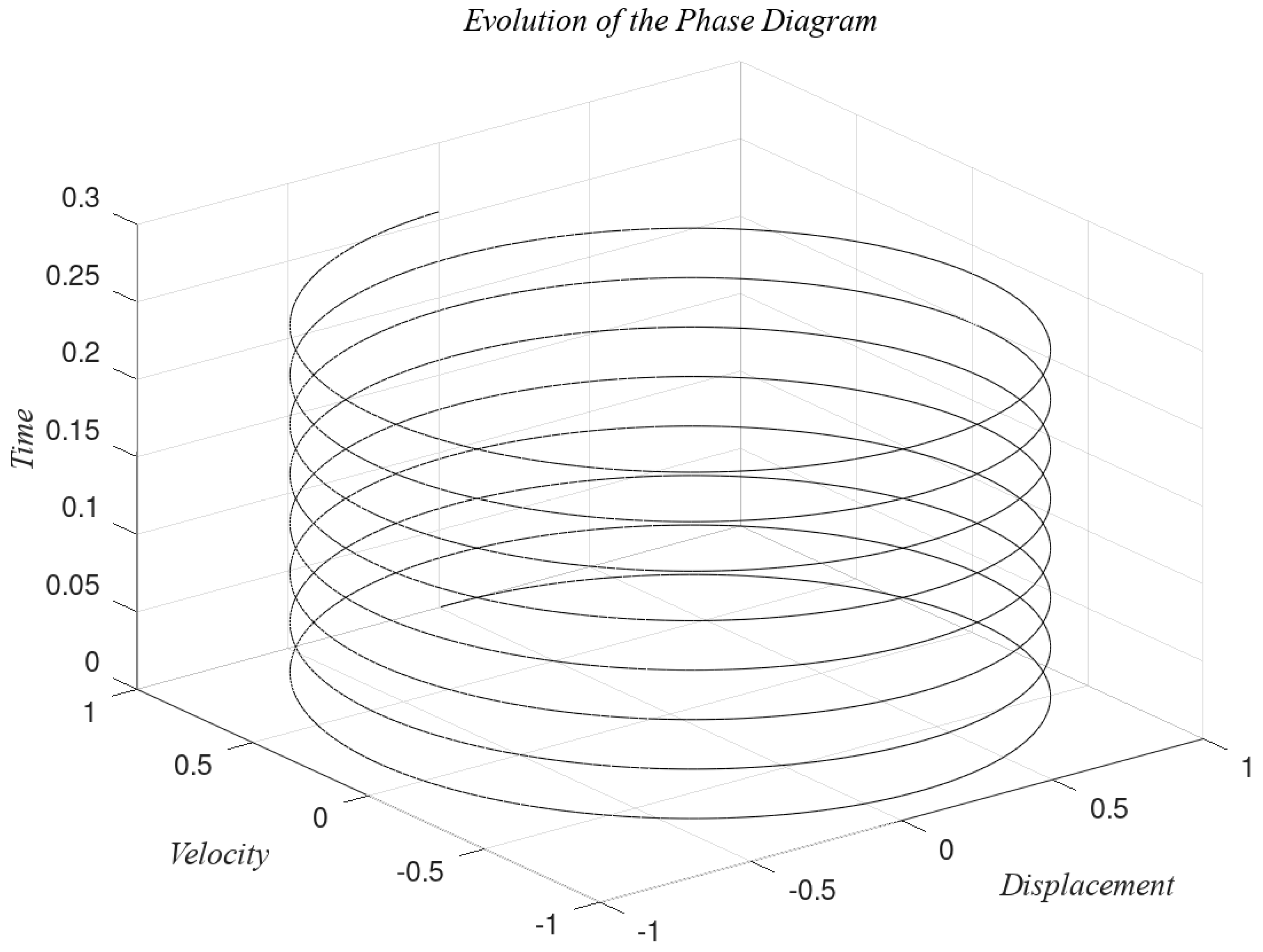
Figure 1. Evolution of a Hamiltonian system.
Machines 13 00233 g001
Figure 2. Phase plane of a Hamiltonian system with steady conditions.
Machines 13 00233 g002
Figure 3. Recurrence plot of a Hamiltonian system with steady conditions.
Machines 13 00233 g003
Figure 4. The experimental wind turbine.
Machines 13 00233 g004
Figure 5. Accelerometer measurements on ten different days.
Machines 13 00233 g005
Figure 6. Magnetometer measurements on ten different days.
Machines 13 00233 g006
Figure 7. Frequency spectrum, acceleration data, case 0.
Machines 13 00233 g007
Figure 8. Spectrogram, acceleration data, case 0.
Machines 13 00233 g008
Figure 9. Frequency spectrum, acceleration data, case 1.
Machines 13 00233 g009
Figure 10. Spectrogram, acceleration data, case 1.
Machines 13 00233 g010
Figure 11. Frequency spectrum, acceleration data, case 2.
Machines 13 00233 g011
Figure 12. Spectrogram, acceleration data, case 2.
Machines 13 00233 g012
Figure 13. Frequency spectrum, acceleration data, case 3.
Machines 13 00233 g013
Figure 14. Spectrogram, acceleration data, case 3.
Machines 13 00233 g014
Figure 15. Recurrence plot of the accelerometer data, case 0.
Machines 13 00233 g015
Figure 16. Recurrence plot of the accelerometer data, case 1.
Machines 13 00233 g016
Figure 17. Recurrence plot of the accelerometer data, case 2.
Machines 13 00233 g017
Figure 18. Recurrence plot of the accelerometer data, case 3.
Machines 13 00233 g018
Figure 19. Frequency spectrum, magnetometer data, case 0.
Machines 13 00233 g019
Figure 20. Spectrogram, magnetometer data, case 0.
Machines 13 00233 g020
Figure 21. Frequency spectrum, magnetometer data, case 1.
Machines 13 00233 g021
Figure 22. Spectrogram, magnetometer data, case 1.
Machines 13 00233 g022
Figure 23. Frequency spectrum, magnetometer data, case 2.
Machines 13 00233 g023
Figure 24. Spectrogram, magnetometer data, case 2.
Machines 13 00233 g024
Figure 25. Frequency spectrum, magnetometer data, case 3.
Machines 13 00233 g025
Figure 26. Spectrogram, magnetometer data, case 3.
Machines 13 00233 g026
Figure 27. Recurrence plot of the magnetometer data, case 0.
Machines 13 00233 g027
Figure 28. Recurrence plot of the magnetometer data, case 1.
Machines 13 00233 g028
Figure 29. Recurrence plot of the magnetometer data, case 2.
Machines 13 00233 g029
Figure 30. Recurrence plot of the magnetometer data, case 3.
Machines 13 00233 g030
Figure 31. Comparison of the recurrence rate with the ideal case. The orange line corresponds to the accelerometer and the blue line to the magnetometer.
Machines 13 00233 g031
Figure 32. Comparison of the determinism with the ideal case. The orange line corresponds to the accelerometer and the blue line to the magnetometer.
Machines 13 00233 g032
Figure 33. Comparison of the laminarity with the ideal case. The orange line corresponds to the ideal condition, the blue line to the magnetometer, and the gray line to the accelerometer.
Machines 13 00233 g033
Figure 34. Comparison of the longest vertical line with the ideal case. The orange line corresponds to the accelerometer and the blue line to the magnetometer.
Machines 13 00233 g034
Figure 35. Comparison of the longest diagonal with the ideal case. The orange line corresponds to the accelerometer and the blue line to the magnetometer.
Machines 13 00233 g035
Figure 36. Comparison of the Shannon entropy with the ideal case. The orange line corresponds to the accelerometer and the blue line to the magnetometer.
Machines 13 00233 g036
Figure 37. Cross-recurrence plot, cases 1 and 2, accelerometer data.
Machines 13 00233 g037
Figure 38. Cross-recurrence plot, cases 1 and 2, magnetometer data.
Machines 13 00233 g038
Table 1. Recurrence quantitative analysis parameters.
RQAEquationDescription
Recurrence Rate R R = 1 N 2 i , j N R i j Determines the average number of recurrence points.
Determinism D E T = l = l m i n N l P l l = 1 N l P l Determines the percentage of points that are on a diagonal. l is the index of each diagonal, and P l is the histogram of the diagonal. A chaotic system has short diagonals, and a periodic system forms regular diagonals, parallel to the main diagonal.
Longest Diagonal L M = max l i Measures the length (in points) of the longest diagonal.
Average Vertical Length T T = v = v m i n N v P v v = v m i n N P v Measures the percentage of recurrence points that lay on a vertical line. v is the index corresponding to the vertical line, and P v is the histogram of the vertical line.
Longest Vertical Line V M = max v i Measures the length of the longest vertical line.
Laminarity L A M = v = v m i n N v P v l = 1 N v P v Measures the percentage of recurrence points that create vertical lines. v is the index of the corresponding vertical line, P v is the histogram of the vertical line.
Shannon Entropy E = 1 N P i L n P i Measures the disorder of the phase plane. For a linear and periodic system, the Shannon entropy is almost zero. For a non-deterministic and noisy system, the Shannon entropy will be almost infinite. P i = P x j = x i is the relative frequency; it is calculated as the ratio of diagonal with non-recurrence points divided by the number of recurrent points.
Table 2. Recurrence quantitative analysis parameters for a Hamiltonian system with a single diagonal.
R R D E T L A M L M T T V M E
0.00050.001498512000110.63651
Table 3. Field case data.
CaseDateWind Condition
016 FebruaryNo
112 AprilYes
224 AprilYes
310 OctoberYes
Table 4. Highest amplitudes of the acceleration data corresponding to the four cases.
Case0123
Amplitude2 × 10−50.001250.00250.0015
Table 5. Highest amplitudes of the magnetometer data corresponding to the four cases.
Case0123
Amplitude0.000450.00210.00250.00125
Disclaimer/Publisher’s Note: The statements, opinions and data contained in all publications are solely those of the individual author(s) and contributor(s) and not of MDPI and/or the editor(s). MDPI and/or the editor(s) disclaim responsibility for any injury to people or property resulting from any ideas, methods, instructions or products referred to in the content.