Development and Validation of a Large Strain Flow Curve Model for High-Silicon Steel to Predict Roll Forces in Cold Rolling

Abstract

Accurately modeling the flow curve over a large strain range is crucial for predicting the flow stress behavior of high silicon steel undergoing strain hardening in the continuous cold rolling process. This study proposes a large strain flow curve model for high-silicon steel, a material commonly used in the cores of electromagnetic devices such as electric motors, generators, and transformers. This model was developed through a series of tensile tests on homogenously pre-strained specimens. Pilot cold rolling was performed at various thickness reduction ratios to impart different magnitudes of pre-strain to sheet-type tensile specimens. The proposed flow curve model was implemented in a VUHARD user-defined subroutine within Abaqus/Explicit, and the predicted roll separating forces were compared with those measured from the pilot cold rolling tests. The comparison demonstrated that the proposed flow curve model accurately captures the flow stress behavior of high-silicon steel at different strain rates over a large strain range, with an R-squared value of 0.9932. The predicted roll separating forces closely matched the measurements from the pilot cold rolling tests, with an average difference of 5.1%.

1. Introduction

The rapid growth of the global electric vehicle market has significantly increased the demand for non-grain-oriented high-silicon steel sheets (Si: 3–3.4%), which are essential for manufacturing laminations in electric motor rotors. These steel sheets (hereafter referred to also as “material”) are typically produced using a single-stand reversing cluster mill, where the sheet thickness is gradually reduced through multiple passes. A “pass” in the rolling process refers to each stage in which the material undergoes deformation between a pair of rolls in a stand. A commonly used cluster mill, the Sendzimir mill [1], features a configuration of two small-diameter work rolls supported by twenty large-diameter backup rolls, which minimizes work roll deflection and reduces vertical elastic deformation of the mill. However, this process has limited productivity due to the reversing nature of the mill.

To improve productivity, there is growing interest in using general continuous four-high cold rolling mills, configured in series with 5–7 stands. Each stand, however, experiences noticeable elastic vertical displacement due to the roll separating force, known as mill stretch (δ = P/M) [2,3,4]. Here, P indicates the roll separating force (referred to as roll force) acting on the material during rolling. All components that compose a rolling mill are subjected to elastic deformation by the roll force [5]. The mill modulus M, or mill stiffness, is defined as the ratio of a known load applied to the measured vertical deformation of the rolling mill, which includes the deformation of the rolls, screw-down device, and housing. The setup roll gap (G_set), the adjusted distance between the upper and lower rolls before rolling begins, is determined by subtracting δ from the reference roll gap (G_ref), also referred to as the design roll gap. Precise calculation of G_set is essential to prevent thickness deviations in continuous cold rolling, ensuring the final product meets required specifications.

As the material strain hardens while passing through multiple stands during the continuous cold rolling process, the roll force at each stand increases, causing a greater δ at each stand, and subsequently widening the roll gap. As mill modulus is an intrinsic property of each stand, accurately estimating the roll force is crucial for determining G_set.

To achieve accurate roll force predictions, a large strain flow curve for the material is needed, which accounts for the material’s strain hardening behavior. The large strain flow curve describes the relationship between stress and strain during plastic deformation at higher strains, typically covering strains up to 1.0.

Several studies have explored the large strain flow curve of silicon steel, often applying it to examine edge cracking during cold rolling. Yan et al. [6] investigated the effects of rolling parameters, such as the tension applied to a 2.5% silicon steel strip, thickness reduction per pass, and the friction coefficient, on edge cracking. Byon et al. [7] further examined how the ratio of work roll barrel length to the radius of curvature of the work roll surface profile influences crack growth direction and length in 3.0% silicon steel. Recently, Roh et al. [8] used finite element (FE) simulations to study edge cracking by altering the secondary work roll bending ratio and initial notch length in 3.4% silicon steel.

However, in works like Yan et al. [6] and Roh et al. [8], true stress-strain curves were only measured through tensile testing up to the necking point (approximately strain of 0.2) and extrapolated up to a strain of 1.0 using empirical hardening equations such as Swift [9] or Voce [10]. Additionally, these studies did not consider strain rate effects on strain hardening, despite the fact that strain rates in cold rolling typically range from 5 s⁻¹ to 40 s⁻¹, where higher strain rates increase material strength.

In this study, a series of tensile tests were performed using pre-strained specimens up to a strain of 0.9 to develop a flow curve model applicable to high-silicon steel (3.4% Si), while incorporating strain rate effects. Pre-straining was introduced in specimens using a reversible pilot cold rolling mill, reducing specimen thickness by various percentages. Standard tensile tests were then performed on these pre-strained specimens to measure the flow stress and equivalent strain at each thickness reduction ratio. To establish a comprehensive flow curve model applicable across a range of strains and strain rates, we integrated two existing models: the Hockett–Sherby flow curve model [11], which effectively describes plastic flow behavior at high strains, and the Johnson–Cook flow curve model [12], a widely used empirical model that accounts for strain, strain rate, and temperature effects.

The resulting large-strain flow curve model was implemented in Abaqus 2017/Explicit via a VUHARD user subroutine, incorporating stress derivatives with respect to strain hardening and strain rate. Finally, we validated the proposed model by comparing roll forces measured in pilot cold rolling tests with those obtained from finite element (FE) analysis, confirming its accuracy and practical applicability.

2. Experimental

Recently, Zheng et al. [13] introduced a non-contact method using digital image correlation (DIC) with laser speckles to evaluate large plastic deformations in thin metals. This technique achieved plastic strains of 0.45 at room temperature and 0.6 at 400 °C, surpassing the strain levels typically measured in conventional uniaxial tensile tests. However, DIC is not suitable for measuring flow stress across a wide strain range.

Coppieters et al. [14] reviewed various methods for acquiring large strain flow curves of metals, categorizing them into three approaches. As concluded by Gil Sevillano et al. [15], the drawing and rolling methods, which fall under the second approach, are ideal for imparting pre-strain to flat- or bar-shaped tensile specimens due to the associated compressive stress states that delay structural damage up to large strains. Byon et al. [16] and Zhuang et al. [17] used cold rolling to introduce plastic strain in their materials.

In this study, we employed the cold rolling method to prepare pre-strained specimens. The cold rolling test configuration for imparting pre-strains to the specimens is shown in Figure 1.

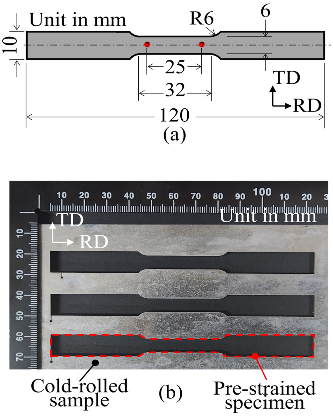
2.1. Preparation of the Test Samples and No-Strained Tensile Specimen

A portion of a 3.4 wt% silicon strip hot-rolled at POSCO was cut out and processed into samples, each with dimensions of 200 mm in length, 150 mm in width, and 2.1 mm in thickness. The samples were then immersed in hydrochloric acid for 1 h to remove the surface scales generated during hot rolling. The central part of one sample was machined into a standard tensile specimen, which will be referred to as the no-strained tensile specimen in this study. This specimen was prepared in accordance with ASTM E8/E8M-16a [18], ensuring that it was not subjected to any additional straining or heating during the machining process.

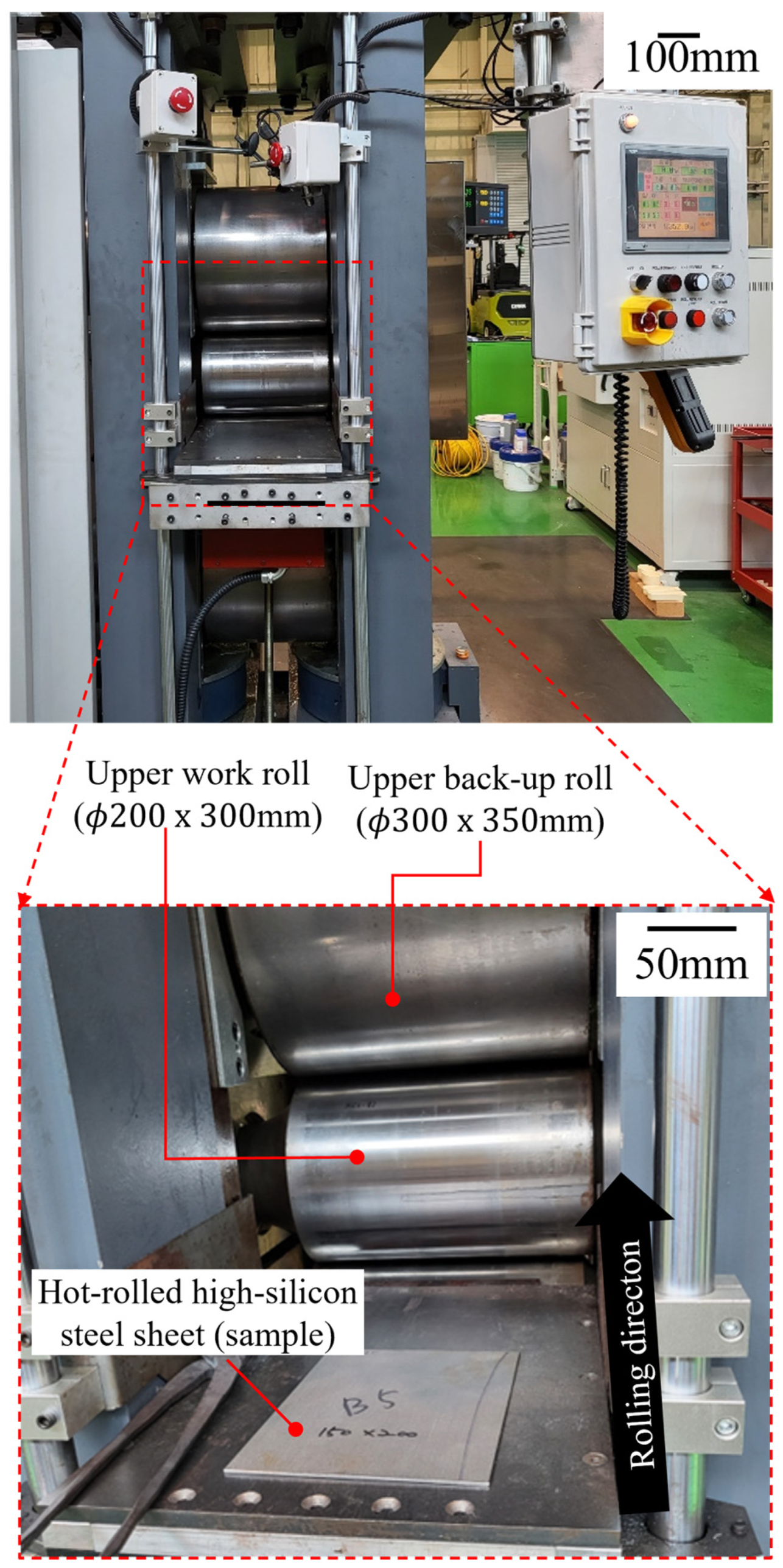
2.2. Pilot Cold Rolling to Prepare Pre-Strained Tensile Specimens

Nine samples were cold rolled at varying thickness reduction ratios to achieve a wide range of pre-strains. Figure 1 shows a four-high reversible pilot cold rolling mill used in this study, with a maximum load capacity of 600 tons and motor power of 300 kW. The work roll had a diameter of 200 mm and a barrel length of 300 mm, while the backup rolls had a diameter of 300 mm and a barrel length of 350 mm. The rolling speed was 9.4 m/min (≈156.7 mm/s). Lubricating oil was applied between the work rolls and the backup rolls only to prevent specimen slippage during rolling.

The samples were cold rolled at various thickness reduction ratios: 12.1%, 15.7%, 22.6%, 23.7%, 29.5%, 32.9%, 33.8%, 42.5%, and 51.6%. After rolling, pre-strained tensile specimens were prepared by machining the central region of each cold-rolled sample according to ASTM E8/E8M standards [19] (Figure 2a). Low-speed wire cutting was employed to prevent thermal deformation and ensure dimensional accuracy (Figure 2b).

2.3. Uniaxial Tensile Test Using a No-Strained (Tensile) Specimen

A uniaxial tensile test was performed on a no-strain specimen using a hydraulic-controlled MTS 370.1 system (maximum load: 100 kN). The specimen had a gauge length of 50 mm, and data were collected at a sampling frequency of 30 Hz. The test was repeated three times to ensure consistency. The crosshead speed was set to 18 mm/min, corresponding to a strain rate of 0.005 s⁻¹, which meets the criteria for quasi-static deformation (strain rate ≤ 0.1 s⁻¹).

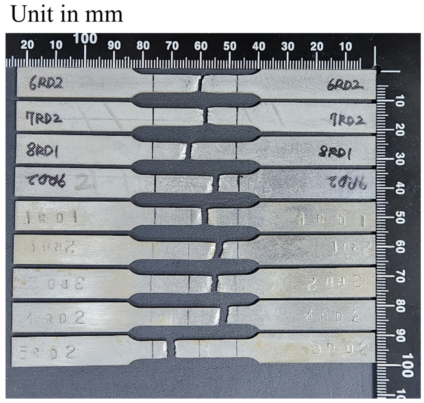
2.4. Uniaxial Tensile Test Using the Pre-Strained (Tensile) Specimens

A uniaxial tensile test was conducted on each pre-strained specimen using a hydraulic-controlled INSTRON-8861 system (Instron, Norwood, MA, USA, maximum load: 300 kN). The gauge length of these specimens was 25 mm, and data acquisition was performed at a sampling frequency of 10 Hz. Each test was repeated twice, and the average values were used to model the flow curve. The loading speed was set to 0.5 mm/min (strain rate = 0.00026 s⁻¹) to minimize potential noise in the stress–strain curve measurements.

Table 1. Summary of calculated plastic stress, strain, and measured ultimate tensile stress.

No	Specimen Thickness, t (mm)	Thickness Reduction Ratio (%)	${\overline{\mathit{\epsilon }}}_{\mathit{p}\mathit{r}\mathit{e}}^{\left(\mathit{n}\right)}$	${\overline{\mathit{\epsilon }}}_{\mathit{p}}^{\left(\mathit{n}\right)}$	${\mathit{\sigma }}_{\mathit{U}\mathit{T}\mathit{S}}^{\left(\mathit{n}\right)}$ (MPa)
0	2.1	0	-	-	663.6
1	1.85	12.1	0.149	0.153	735.6
2	1.77	15.7	0.198	0.204	743.6
3	1.62	22.6	0.296	0.303	810.8
4	1.60	23.7	0.312	0.316	805.6
5	1.48	29.5	0.416	0.421	835.8
6	1.41	32.9	0.459	0.464	853.3
7	1.39	33.8	0.472	0.479	856.7
8	1.21	42.5	0.643	0.664	892.7
9	1.02	51.6	0.832	0.837	913.6

${\overline{\epsilon }}_p^{\left(n\right)}$: calculated equivalent plastic strain, ${\overline{\epsilon }}_{pre}^{\left(n\right)}$: calculated prestrain, and ${\sigma }_{UTS}^{\left(n\right)}$: measured ultimate tensile stress where n denotes number.

summarizes the calculated equivalent plastic strain, pre-strain, ultimate tensile stress (UTS), and specimen thickness at each thickness reduction ratio. “No 0” means the state without strain hardening. The thickness listed in column 2 is the thickness of specimens used for the next rolling test. Thickness is measured before the rolling test at each reduction ratio. For example, if the initial specimen thickness is 2.1 mm and it is rolled at a reduction ratio of 12.1%, the specimen thickness becomes 1.85 mm, as shown in column 2. Figure 3 shows the pre-strained specimens after the uniaxial tensile tests were completed.

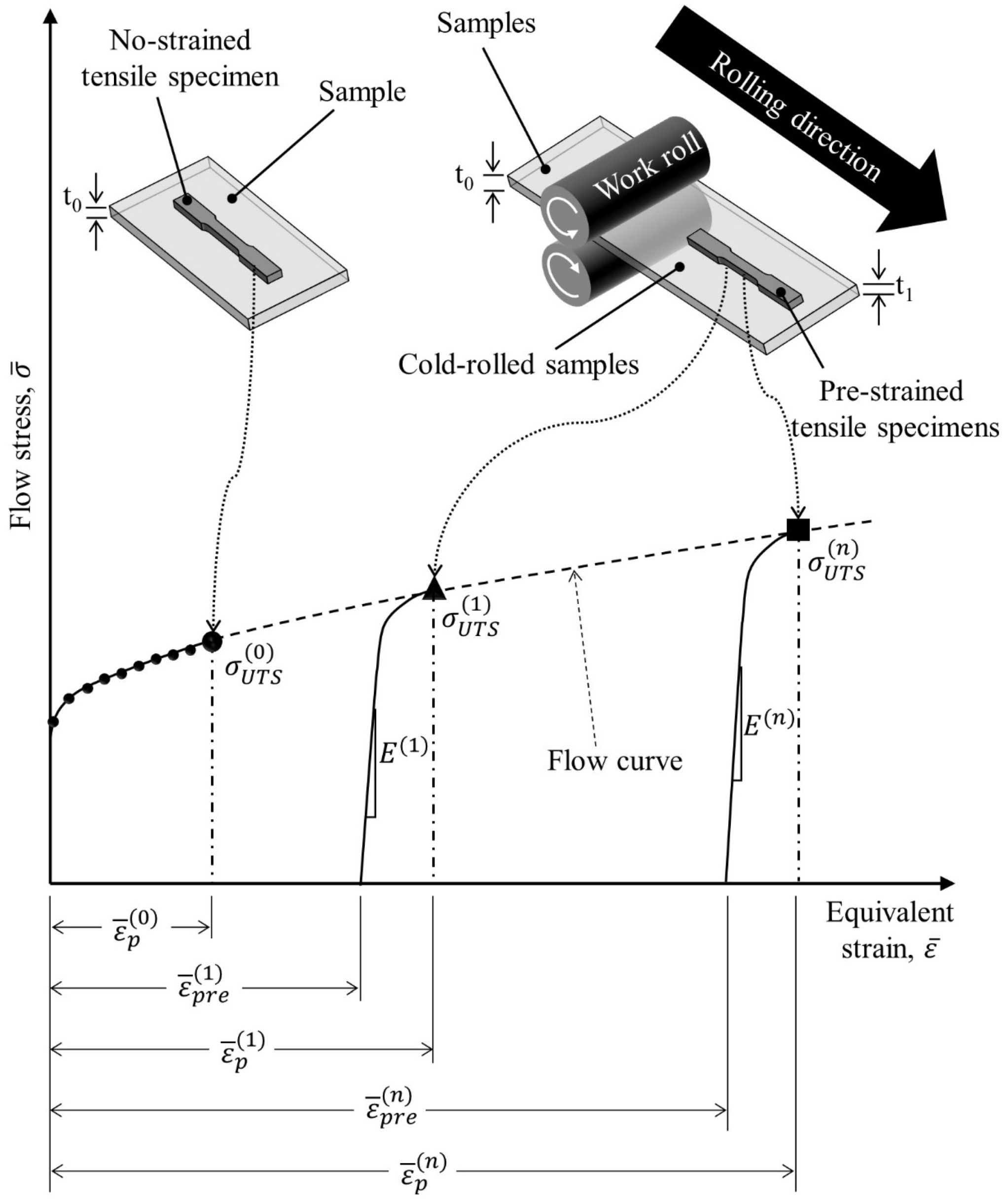
3. Construction of a Large Strain Flow Curve of High-Silicon Steel

The flow curve represents the relationship between flow stress ($\overline{\sigma }$) and equivalent strain ($\overline{\epsilon }$) during plastic deformation, excluding elastic strain. The steps involved in constructing a large strain flow curve are explained below along with Figure 4.

(i)

Uniaxial tensile test on no-strain specimen

A uniaxial tensile test was conducted on the no-strain specimen to measure the flow stress-equivalent strain curve up to necking (represented by solid black circles).

(ii)

Calculation of equivalent strain for pre-strained specimens

The equivalent strain accumulated in the pre-strained specimens due to strain hardening from cold rolling was calculated as [20]:

$$\overline{\epsilon }=\sqrt{{\displaystyle \frac{2}{3}}\left({{\epsilon }_{thick}}^2+{{\epsilon }_{length}}^2+{{\epsilon }_{width}}^2\right)}$$

(1)

with incompressibility condition [20]:

$${\epsilon }_{thick}+{\epsilon }_{length}+{\epsilon }_{width}=0$$

(2)

where ${\epsilon }_{thick}$,${\epsilon }_{length}$, and ${\epsilon }_{width}$ are the principal strains in the thickness, longitudinal, and transverse directions, respectively. Due to the plane strain condition, ${\epsilon }_{width}\approx 0$.

(iii)

Calculation of pre-strain (${\overline{\epsilon }}_{pre}$)

The pre-strain in the pre-strained specimens was calculated as [20]:

$${\overline{\epsilon }}_{pre}=\sqrt{{\displaystyle \frac{2}{3}}\left({{\epsilon }_{thick}}^2+{\left(-{\epsilon }_{thick}\right)}^2\right)}={\displaystyle \frac{2}{\sqrt{3}}}{\epsilon }_{thick}$$

(3)

where ${\epsilon }_{thick}=\left| ln\left({\displaystyle \frac{t_0}{t_f}}\right)\right|$ and $t_0$ and $t_f$ represent the initial and final thicknesses of the specimen, respectively.

(iv)

Calculation of equivalent plastic strain (${\overline{\epsilon }}_p$)

For the first pre-strained specimen, the equivalent plastic strain was computed as [20]:

$${\overline{\epsilon }}_p^{\left(1\right)}={\overline{\epsilon }}_{tot}^{\left(1\right)}-{\overline{\epsilon }}_e^{\left(1\right)}+{\overline{\epsilon }}_{pre}^{\left(1\right)}$$

(4)

where ${\overline{\epsilon }}_e^{ \left(1\right)}={\displaystyle \frac{{\sigma }_{YS}^{\left(1\right)}}{E^{\left(1\right)}}} , {\sigma }_{YS}^{\left(1\right)}$ is the yield stress (YS) and $E^{\left(1\right) }$ is Young’s modulus. The superscript denotes the number of rolling passes. The measured UTS (solid black triangle) and calculated plastic strain were marked on the flow curve in Figure 4. ${\overline{\epsilon }}_{tot}^{ \left(1\right) }$ is the total equivalent strain, and ${\overline{\epsilon }}_e^{\left(1\right) }$ is the equivalent elastic strain.

(v)

Repetition for all pre-strained specimens

Steps (ii)–(iv) were repeated for pre-strained specimens. The measured UTS and calculated pre-strains were then plotted to build the flow curve.

(vi)

Flow curve construction using curve-fitting method

A large strain flow curve was constructed by connecting the data $\left({\sigma }_{UTS}^{\left(0\right)}, {\sigma }_{UTS}^{\left(1\right)}, \mathrm{and} {\sigma }_{UTS}^{\left(n\right)}\right)$ and using a mathematical curve-fitting model.

4. Rate-Dependent Flow Stress Behavior and FE Implementation

Strain hardening is a phenomenon in which the flow stress required for plastic deformation increases with an increase in strain, especially when the metal is deformed at varying strain rates and temperatures. In this study, the effect of temperature on flow stress was ignored because the temperature change during pilot cold rolling was negligible. Among various strain rate-dependent flow stress models, the Johnson–Cook (J–C) model [12] is widely used. In the J–C model, flow stress at room temperature is represented as a product of a strain hardening term and a strain rate term:

$${\overline{\sigma }}_{J-C}=\left\{A_1+A_2\ast {\overline{\epsilon }}_p^{ A_3}\right\}\left[1+A_4\ast ln\left({\displaystyle \frac{\dot{\overline{\epsilon }}}{{\dot{\overline{\epsilon }}}_0}}\right)\right]$$

(5)

where the term in curly braces represents strain hardening and the term in square brackets denotes the strain rate effect. The sign strain rate is positive. $A_{1 }$ is the yield stress at a reference strain rate, $A_{2 }$ is the coefficient of strain hardening, $A_{3 }$ is the strain hardening exponent, and $A_{4 }$ is the coefficient of strain rate. ${\dot{\overline{\epsilon }}}_0$ is the reference strain rate, and 0.005 s⁻¹ was used in this study.

4.1. Proposed Flow Curve Model

This study proposes a flow curve model suitable for various strains and strain rates by combining the Hockett–Sherby model [11] and the Johnson–Cook model [12]:

$${\overline{\sigma }}_{proposed}=\left\{B_1-B_{2}exp\left(-B_3{\overline{\epsilon }}_p^{ B_4}\right)\right\}\left[1+B_5 ln\left({\displaystyle \frac{\dot{\overline{\epsilon }}}{{\dot{\overline{\epsilon }}}_0}}\right)+B_6{\left(ln\left({\displaystyle \frac{\dot{\overline{\epsilon }}}{{\dot{\overline{\epsilon }}}_0}}\right)\right)}^2\right]$$

(6)

where $B_{1 }$ to $B_{4 }$ are material constants related to strain hardening, while $B_5$ to $B_6$ account for the strain rate effects. The term in curly braces, originally proposed by Hockett and Sherby [11], describes the strain hardening. To capture the effect of strain rate on flow stress, the J–C model [12] was modified as shown in square brackets. Constants $B_1$ to $B_4$ were determined using genetic algorithms [21,22] to minimize the error between the measured and calculated flow stresses. The constants $B_5$ and $B_6$ were obtained by rearranging Equation (6) as:

$${\displaystyle \frac{{\overline{\sigma }}_{propsed}}{B_1-B_{2}exp\left(-B_3{\overline{\epsilon }}^{ B_4} \right)}}-1=B_5 ln\left({\displaystyle \frac{\dot{\overline{\epsilon }}}{{\dot{\overline{\epsilon }}}_0}}\right)+B_6{\left(ln\left({\displaystyle \frac{\dot{\overline{\epsilon }}}{{\dot{\overline{\epsilon }}}_0}}\right)\right)}^2$$

(7)

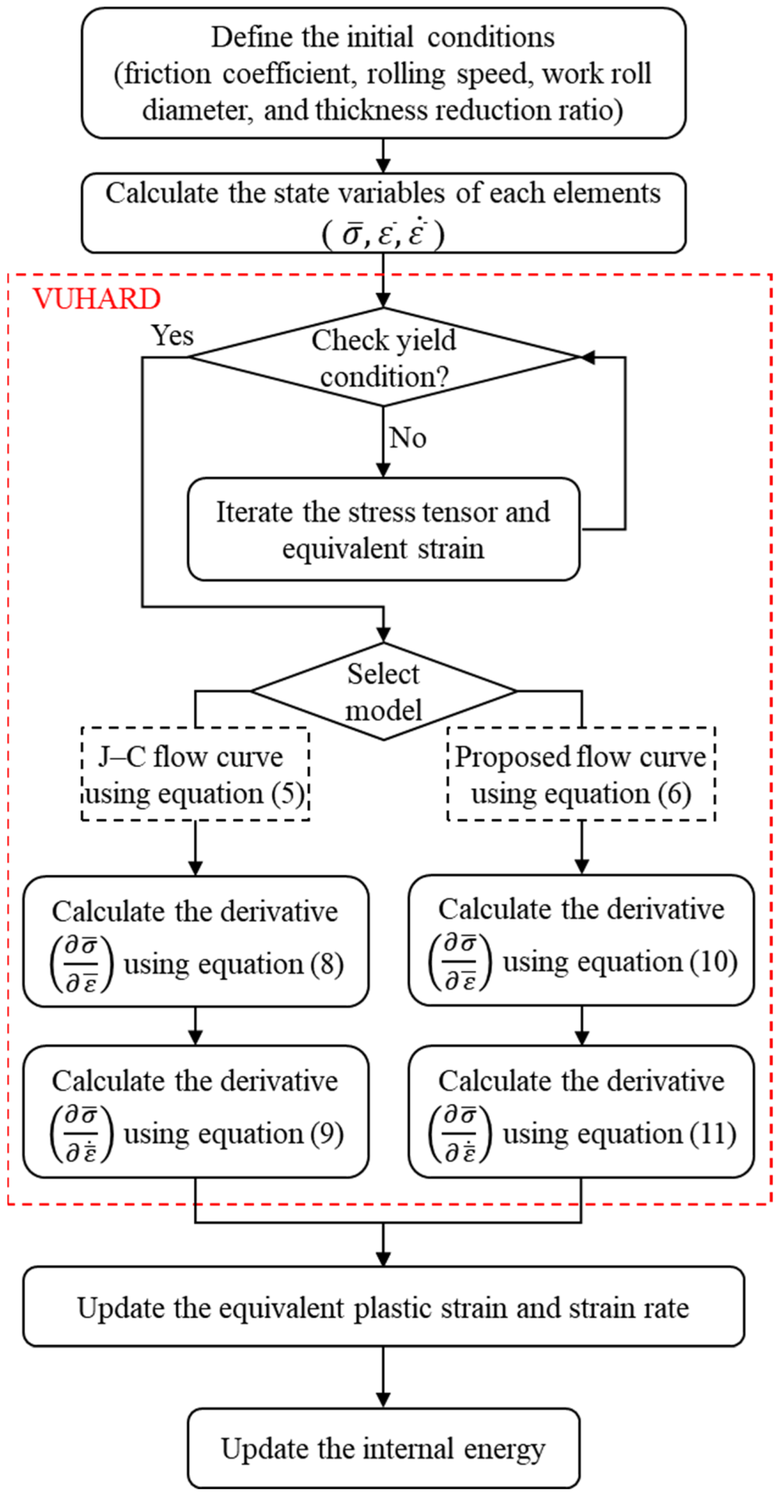
4.2. Implementation of VUHARD

The Abaqus/Explicit material library [23] lacks support for derivatives of yield stress concerning strain and strain rate, as required for implementing the J–C and proposed models. A user subroutine, VUHARD, was coded to handle these derivatives, one for stress due to strain hardening $\left(={\displaystyle \frac{\partial \overline{\sigma }}{\partial \overline{\epsilon }}}\right)$ and another for stress as a function of strain rate $\left(={\displaystyle \frac{\partial \overline{\sigma }}{\partial \dot{\overline{\epsilon }}}}\right)$. These derivatives represent changes in total flow stress with respect to equivalent plastic strain rate and equivalent plastic strain [24]. The strain components were updated using the associate flow rule, as illustrated in the VUHARD subroutine flowchart in Figure 5.

In the J–C model, the derivatives are:

$${\displaystyle \frac{\partial {\overline{\sigma }}_{J-C}^{\left(k+1\right)}}{\partial {\overline{\epsilon }}^{\left(k+1\right)}}}=A_2{A}_3{\left({\overline{\epsilon }}^{\left(k+1\right)}\right)}^{ \left(A_3-1\right)}$$

(8)

$${\displaystyle \frac{\partial {\overline{\sigma }}_{J-C}^{\left(k+1\right)}}{\partial {\dot{\overline{\epsilon }}}^{\left(k+1\right)}}}={\displaystyle \frac{A_4}{{\dot{\overline{\epsilon }}}_0}}$$

(9)

where k is the iteration number.

For the flow curve model proposed, the derivatives are:

$${\displaystyle \frac{\partial {\overline{\sigma }}_{proposed}^{\left(k+1\right)}}{\partial {\overline{\epsilon }}^{\left(k+1\right)}}}=B_2{B}_3{B}_4{\left({\overline{\epsilon }}^{\left(k+1\right)}\right)}^{ \left(B_4-1\right)}exp\left(-B_3{\left({\overline{\epsilon }}^{\left(k+1\right)}\right)}^{ B_4}\right)$$

(10)

$${\displaystyle \frac{\partial {\overline{\sigma }}_{propsed}^{\left(k+1\right)}}{\partial {\dot{\overline{\epsilon }}}^{\left(k+1\right)}}}=\left(B_5+2B_{6}ln\left({\displaystyle \frac{{\dot{\overline{\epsilon }}}^{\left(k+1\right)}}{{\dot{\overline{\epsilon }}}_0}}\right)\right)/{\dot{\overline{\epsilon }}}_0$$

(11)

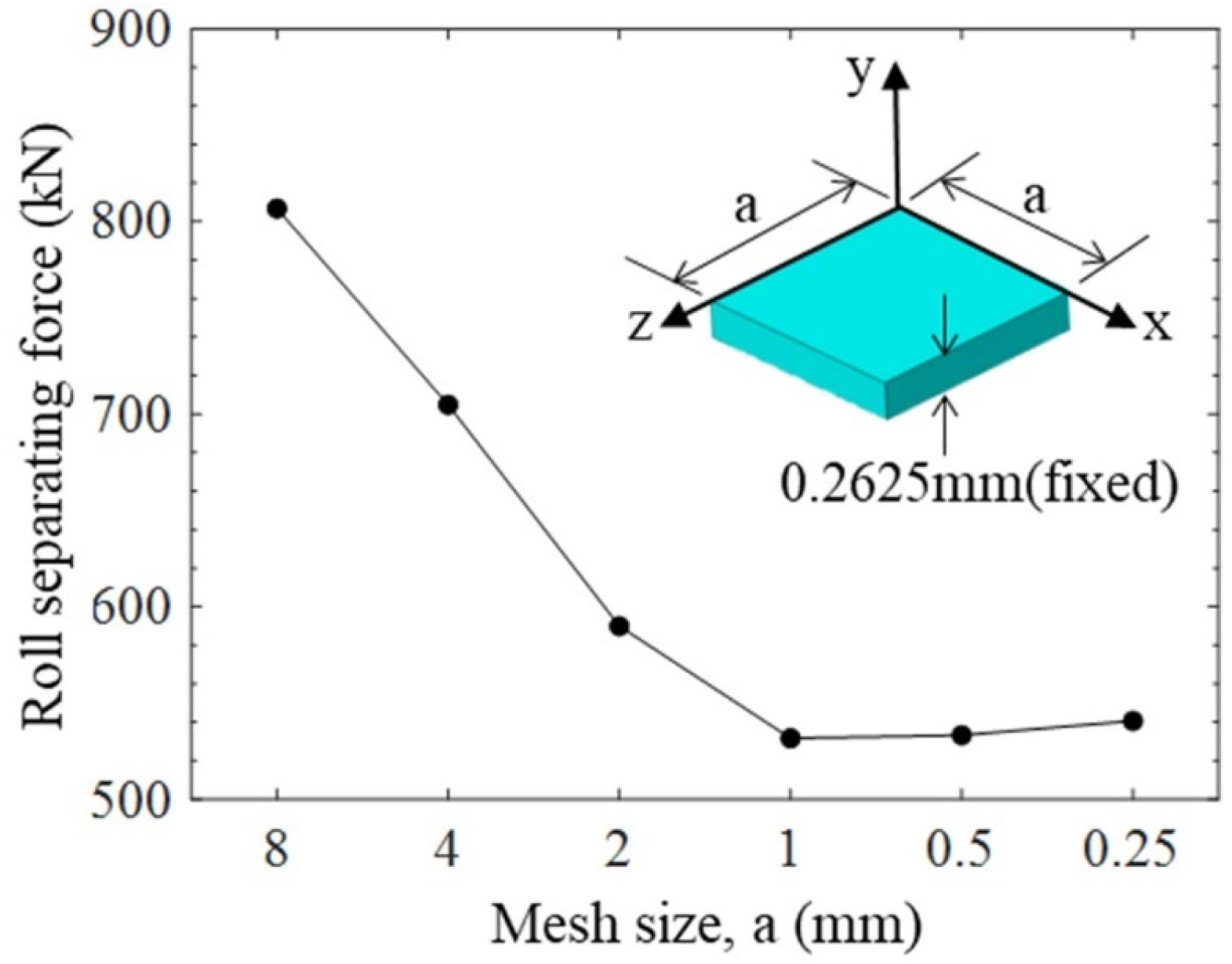
4.3. Boundary Conditions and Mesh

FE analyses with von Mises plasticity were carried out using Abaqus/Explicit. A half-symmetric model of the work roll and a quarter-symmetric model of the specimen were used to shorten the runtime. The work roll was modeled as an analytic rigid body. Figure 6 illustrates the mesh and boundary conditions applied to both the specimen and the work roll. A 150 mm × 2.1 mm (width × thickness) specimen was meshed with the C3D8R element (an eight-node reduced integrated brick element). The variables $u_n, u_t, {\sigma }_n$, and ${\sigma }_t$ represent the normal displacement, tangential displacement, normal surface traction, and tangential surface traction, respectively. The work roll diameter was 200 mm, barrel length 300 mm, and rolling speed 156.7 mm/s. Coulomb friction condition was used at the interface of the work roll and specimen.

The elastic modulus of the strip was 160 GPa, the density 7290 kg/m³, and the Poisson’s ratio 0.3. A mesh convergence study determined an optimal element size of 1 mm × 0.2625 mm × 1 mm in the x, y, and z directions, respectively, for the thin specimen. Figure 7 illustrates roll force variation as a function of element size, with a total of 73,500 elements used in the FE analyses.

5. Results and Discussion

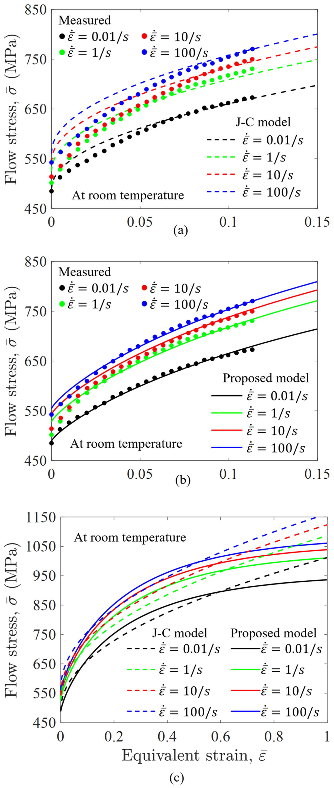
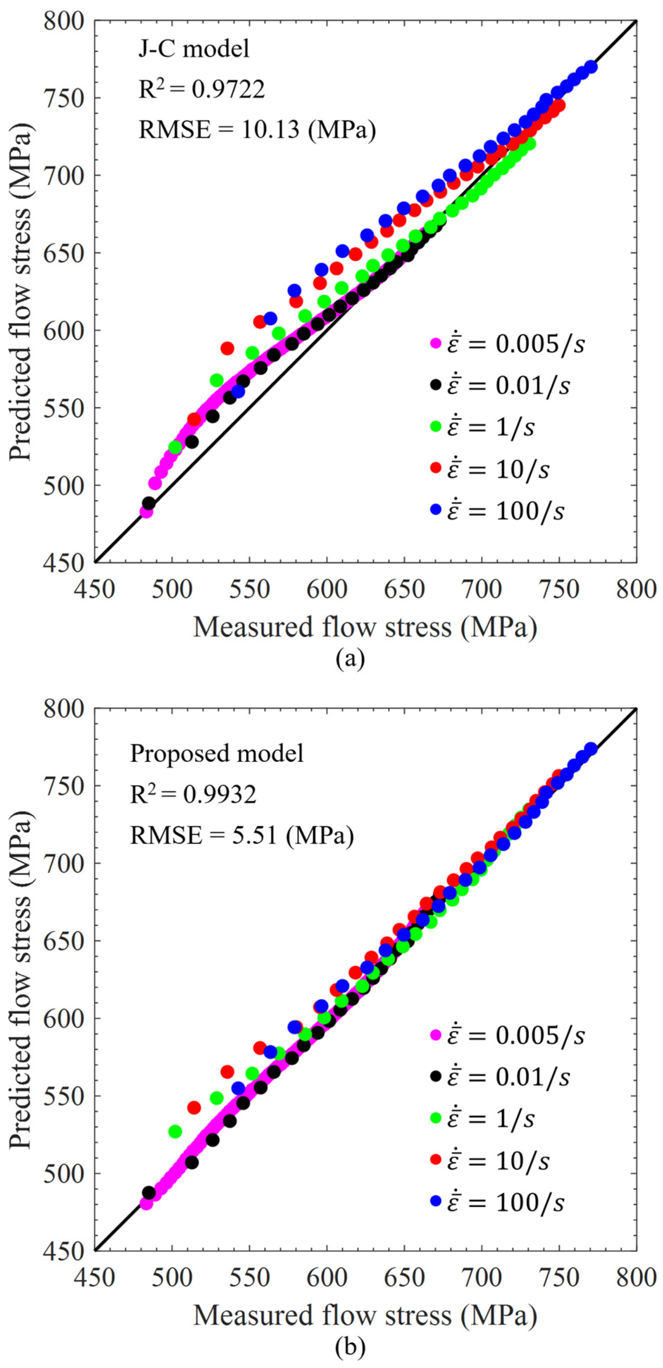
5.1. Large Strain Flow Curve of High-Silicon Steel

Figure 8a presents the measured flow stress-equivalent strain data for a no-strain specimen (black circles) and those for nine pre-strained specimens (black triangles). The Johnson–Cook (J–C) model demonstrates limitations by overestimating flow stress in the strain interval 0 to 0.05, underestimating in the 0.15 to 0.5 range and overestimating beyond 0.65. This indicates that the J–C model is not ideal for capturing the strain-hardening behavior of high-silicon steel over a large strain range. Conversely, Figure 8b shows that the proposed flow curve model effectively captures strain hardening up to an equivalent strain of 0.9.

At large equivalent strains, metals often reach a strain-hardening saturation point, meaning further plastic deformation does not significantly increase stress. Therefore, the proposed model in Figure 8b does not fully capture this saturation effect. This study evaluated the strain rate effect on strain hardening using the data reported by Kwon [25], who performed standard tensile tests on high-silicon steel (Si: 3.4%) over wide ranges of strain rate (0.01–100 s⁻¹) across strain rates from 0.01 s⁻¹ to 100 s⁻¹, using a high-speed testing machine developed by KAIST [26]. Figure 9 illustrates the influence of strain rate on flow stress, and

Table 2. Material constants used in the two large strain flow curve models.

J–C Model		Proposed Model
${\mathrm{A}}_1$	483 (MPa)	${\mathrm{B}}_1$	948.4 (MPa)
${\mathrm{A}}_2$	517.4 (MPa)	${\mathrm{B}}_2$	467.7 (MPa)
${\mathrm{A}}_3$	0.4835	${\mathrm{B}}_3$	2.948
${\mathrm{A}}_4$	0.0162	${\mathrm{B}}_4$	0.7967
		${\mathrm{B}}_5$	0.02118
		${\mathrm{B}}_6$	−0.0005658

outlines the constants used in both J–C and proposed models.

In Figure 9a, the flow stresses and equivalent strains measured at different strain rates are compared to the curves generated by the J–C model. J–C model predictions are inaccurate for strains below 0.06 at strain rates of 0.01 s⁻¹ and 1 s⁻¹, and below 0.08 at rates of 10 s⁻¹ and 100 s⁻¹, suggesting that it does not accurately capture high-silicon steel behavior across strain rates. In Figure 9b, the flow stresses and equivalent strains measured at different strain rates are compared to the curves generated by the proposed flow curve model. Except for slight discrepancies in the strain intervals around ~0.01 for $\dot{\overline{\epsilon }}=1$ s⁻¹ and 10 s⁻¹, and ~0.02 for $\dot{\overline{\epsilon }}$= 100 s⁻¹, the proposed model aligns well with measured data. This is due to the incorporation of both strain hardening and strain rate effects in the proposed model.

For a direct comparison of the two models over a large strain range, the flow stress-equivalent strain curves at different strain rates are presented in Figure 9c. The flow stress increases non-proportionally as the strain rate increases. The proposed flow curve model produces a steeper strain hardening slope in the initial interval of equivalent strain compared to the J–C model, but this slope decreases when the equivalent strain reaches approximately 0.6.

Figure 10 compares the measured and predicted flow stresses for both models. The x-axis represents the measured flow stress and the y-axis represents the predicted flow stress. The model accuracy was assessed using the root mean squared error (RMSE):

$$RMSE=\sqrt{{\displaystyle \frac{1}{m}}{\displaystyle \sum _{i=1}^m}{\left({\overline{\sigma }}^{meas}-{\overline{\sigma }}^{pred}\right)}^2}$$

(12)

where ${\overline{\sigma }}^{means}$ and ${\overline{\sigma }}^{pred}$ denote the measured and predicted flow stresses, respectively, and m is the number of data points. The RMSE was 10.13 MPa for the J–C model and 5.51 MPa for the proposed flow curve model, indicating that the proposed model is approximately 1.84 times more accurate. In Figure 10b, the data marked with red, green, and blue symbols still deviate from proposed model at flow stress values below 600 MPa on the x-axis. This might be attributed to the fact that the proposed model may not accurately capture strain rate effects in the low-stress regime. At low stress values, materials typically undergo elastic or early plastic deformation, where strain rate effects are weaker compared to high-stress conditions [27].

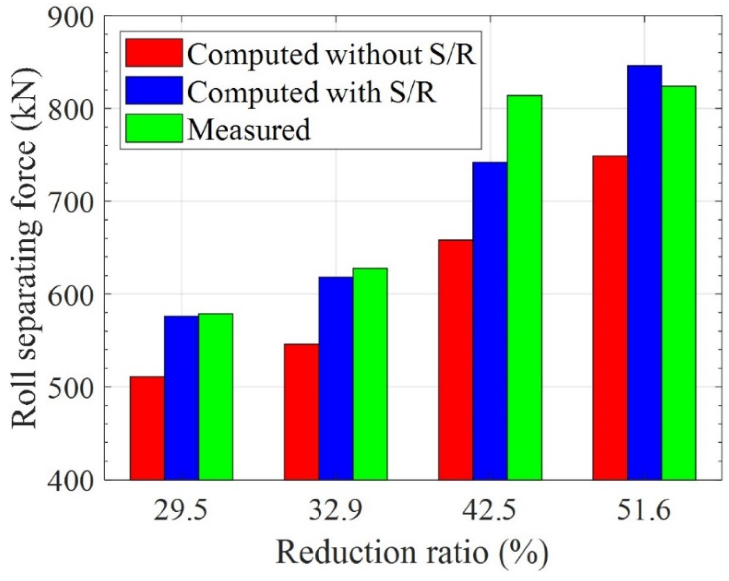
5.2. Application to Predict the Roll Force During Cold Rolling

In multi-pass cold rolling, the strain rates vary with each pass. Therefore, a strain rate-sensitive flow curve model is essential for accurately predicting the roll force. Figure 11 compares roll force values measured in pilot cold rolling with those predicted by the proposed model. “Computed with S/R” includes strain rate effects, while “computed without S/R” excludes them. The specimen dimensions used in the pilot cold rolling test were the same as those described in the “Experimental” section.

When strain rate effects were considered, the prediction error decreased from 9.1–19.2% to 1.3–8.9%. It should be mentioned that the roll force measured at a 42.5% thickness reduction ratio was close to that at 51.6% thickness reduction ratio, which is difficult to explain. This discrepancy may be due to an error in measuring the roll force at the 42.5% thickness reduction ratio.

Table 3. Comparison between the calculated and measured roll separating forces at each thickness reduction ratio (TRR), with and without considering the strain rate effect.

TRR (%)	Measured (kN)	Calculated w/o Strain Rate (kN)	Diff (%)	Calculated with Strain Rate (kN)	Diff (%)
29.5	583.7	511.1	12.4	576.1	1.3
33.8	608.2	545.7	10.3	618.4	1.7
42.4	814.2	658.2	19.2	742.0	8.9
51.4	824.0	748.7	9.1	846.0	2.7

summarizes the calculated and measured roll forces at different thickness reductions, demonstrating that the proposed flow curve model can effectively predict the roll force of high-silicon steel and subsequently calibrate mill stretch of each stand in a general continuous cold rolling mill.

6. Conclusions

Pilot cold rolling was conducted at different thickness reduction ratios to introduce various pre-strains in high-silicon steel sheet specimens. A series of tensile tests was conducted with the pre-strained specimens, and the flow stresses for a wide range of strains were measured. Based on these measurements, a flow curve model functional across various strains and strain rates was developed by combining the Hocket–Sherby flow and Johnson–Cook flow curve models. The proposed flow curve model was implemented into a VUHARD user-defined subroutine of Abaqus/Explicit to compute the roll force during cold rolling; the effectiveness of the strain rate-sensitive flow curve model was verified by comparing the measured roll forces with the predicted values. The following conclusions can be drawn.

• The combination of the Hocket–Sherby and J–C models effectively generate a flow curve suitable for high-silicon steel over large strain ranges.
• The flow curve model proposed in this study can compute the roll force of high-silicon steel during cold rolling, enabling accurate mill stretch estimation and setup roll gap determination.
• FE analysis coupled with the proposed flow curve model accurately simulates the plastic deformation behavior of high-silicon steel, accounting for strain hardening and strain rate effects during cold rolling.

References

1. Winters, G.L.; Nutt, M.J. Stainless Steels for Medical and Surgical Applications; ASTM International: Montgomery, AL, USA, 2003. [Google Scholar]
2. Kucsera, P.; Béres, Z. Hot rolling mill hydraulic gap control (HGC) thickness control improvement. Acta Polytech. Hung. 2015, 12, 93–106. [Google Scholar]
3. Zhang, F.; Zhang, Y.; Chen, H. Automatic gauge control of plate rolling mill. Int. J. Control Autom. 2016, 9, 143–156. [Google Scholar] [CrossRef]
4. Radionov, A.A.; Gasiyarov, V.R.; Karandaev, A.S.; Loginov, B.M.; Khramshin, V.R. Advancement of roll-gap control to curb the camber in heavy-plate rolling mills. Appl. Sci. 2021, 11, 8865. [Google Scholar] [CrossRef]
5. An Introduction to Iron and Steel Processing. Available online: https://www.jfe-21st-cf.or.jp/index2.html (accessed on 14 March 2025).
6. Yan, Y.; Sun, Q.; Chen, J. The initiation and propagation of edge cracks of silicon steel during tandem cold rolling process based on the Gurson-Tvergaard-Needleman damage model. J. Mater. Process. Technol. 2013, 213, 598–605. [Google Scholar] [CrossRef]
7. Byon, S.M.; Roh, Y.H.; Yang, Z.; Lee, Y. A roll-bending approach to suppress the edge cracking of silicon steel in the cold rolling process. Proc. IMechE Part B J. Eng. Manuf. 2021, 235, 112–124. [Google Scholar] [CrossRef]
8. Roh, Y.H.; Byon, S.M.; Lee, Y. Numerical analysis of edge cracking in high-silicon steel during cold rolling with 3D fracture locus. Appl. Sci. 2021, 11, 8408. [Google Scholar] [CrossRef]
9. Swift, H.W. Plastic instability under plane stress. J. Mech. Phys. Solids 1952, 1, 1–18. [Google Scholar] [CrossRef]
10. Voce, E. The relationship between stress and strain for homogeneous deformation. J. Inst. Met. 1948, 74, 537–562. [Google Scholar]
11. Hockett, J.E.; Sherby, O.D. Large strain deformation of polycrystalline metals at low homologous temperatures. J. Mech. Phys. Solids 1975, 23, 87–98. [Google Scholar] [CrossRef]
12. Johnson, G.R.; Cook, W.H. Fracture characteristics of three metals subjected to various strains, Strain rates, temperatures and pressures. Eng. Fract. Mech. 1985, 21, 31–48. [Google Scholar] [CrossRef]
13. Zheng, Q.; Mashiwa, N.; Furushima, F. Evaluation of large plastic deformation for metals by a non-contacting technique using digital image correlation with laser speckles. Mater. Des. 2020, 191, 108626. [Google Scholar] [CrossRef]
14. Coppieters, S.; Traphöner, H.; Stieber, F.; Balan, T.; Kuwabara, T.; Tekkaya, A.E. Large strain flow curve identification for sheet metal. J. Mater. Process. Technol. 2022, 308, 117725. [Google Scholar] [CrossRef]
15. Sevillano, J.G.; Houtte, P.V.; Aernoudt, E. Large strain work hardening and textures. Prog. Mater. Sci. 1980, 25, 69–134. [Google Scholar] [CrossRef]
16. Byon, S.M.; Kim, S.I.; Lee, Y. A numerical approach to determine flow stress-strain curve of strip and friction coefficient in actual cold rolling mill. J. Mater. Process. Technol. 2008, 201, 106–111. [Google Scholar] [CrossRef]
17. Zhuang, X.; Zhao, Z.; Li, H.; Xiang, H. Experimental methodology for obtaining the flow curve of sheet materials in a wide range of strains. Steel Res. Int. 2013, 84, 146–154. [Google Scholar] [CrossRef]
18. ASTM E8/E8M-16a; Standard Test Methods for Tension Testing of Metallic Materials. ASTM International: West Conshohocken, PA, USA, 2020.
19. ASTM E8/E8M; Standard Test Methods for Tension Testing of Metallic Materials. ASTM International: West Conshohocken, PA, USA, 2024.
20. Lee, Y. Rod and Bar Rolling: Theory and Applications; Marcel Dekker, Inc.: New York, NY, USA, 2004. [Google Scholar]
21. Huang, C.; Jiaodong, X.; Zhang, Z. A modified back propagation artificial neural network model based on genetic algorithm to predict the flow behavior of 5754 aluminum alloy. Materials 2018, 11, 855. [Google Scholar] [CrossRef] [PubMed]
22. Chen, G.; Ren, C.; Yu, W.; Yang, X.; Zhang, L. Application of genetic algorithms for optimizing the Johnson–Cook constitutive model parameters when simulating the titanium alloy Ti-6Al-4V machining process. Proc. IMechE Part B J. Eng. Manuf. 2012, 226, 1287–1297. [Google Scholar] [CrossRef]
23. Abaqus 6.14 Documentation. Available online: http://62.108.178.35:2080/v6.14/index.html (accessed on 14 March 2025).
24. Muiruri, A.; Maringa, M.; Preez, W.D. Development of VUMAT and VUHARD subroutines for simulating the dynamic mechanical properties of additively manufactured Parts. Materials 2022, 15, 372. [Google Scholar] [CrossRef] [PubMed]
25. Kwon, J. Semi-Empirical Model Considering the Strain Rate and Grain Size for the Ductile to Brittle Transition Temperature of High Si Electrical Materials. Ph.D. Thesis, Korea Advanced Institute of Science & Technology, Daejeon, Republic of Korea, 2017. [Google Scholar]
26. Huh, H.; Lim, J.; Park, S.H. High speed tensile test of materials for the stress-strain curve at the intermediate strain rate. Int. J. Automot. Technol. 2009, 10, 195–204. [Google Scholar] [CrossRef]
27. Jia, X.; Hao, K.; Luo, Z.; Fan, Z. Plastic deformation behavior of metal materials: A Review of Constitutive Models. Metals 2022, 12, 2077. [Google Scholar] [CrossRef]
Figure 1. A four-high cold rolling mill and hot-rolled high-silicon steel sheet (sample) used in this study.
Machines 13 00243 g001
Figure 2. (a) Dimensions of the pre-strained specimen (ASTM E8/E8M) and (b) traces of pre-strained tensile specimens taken from a sample.
Machines 13 00243 g002
Figure 3. Appearance of nine pre-strained tensile specimens after completing the tensile tests at different thickness reduction ratio (TRR) (12.1%, 15.7%, 22.6%, 23.7%, 29.5%, 32.9%, 33.8%, 42.5%, and 51.6%).
Machines 13 00243 g003
Figure 4. Schematic diagram for constructing the flow curve using multiple pre-strained tensile specimens and a series of uniaxial tensile tests. The small black circles in the beginning represent the measured true stress before necking using the no-strained tensile specimen.
Machines 13 00243 g004
Figure 5. Flowchart for implementing the J–C flow curve model and the proposed flow curve model in Abaqus/Explicit.
Machines 13 00243 g005
Figure 6. Mesh and boundary conditions used for the specimen (material) and work roll.
Machines 13 00243 g006
Figure 7. Variations in roll separating force as a function of mesh (element) size. The X-Z plane element is in contact with the work roll.
Machines 13 00243 g007
Figure 8. Measured large strain flow curve. (a) Comparison of the curve fitting quality between the J–C flow curve model [12] and (b) the proposed flow curve model. Symbol ● represents stress–strain data measured using a no-strained specimen and ▲ stands for the ultimate tensile stress measured using pre-strained specimens.
Machines 13 00243 g008
Figure 9. Effect of strain rate on the flow stress. (a) Measured large strain flow curves [25] are compared with the curve generated from J–C model [12]; (b) proposed model; and (c) large strain flow curves generated from both J–C model [12] proposed model are compared.
Machines 13 00243 g009
Figure 10. Scatter plots of the measured versus predicted flow stress at different strain rates (a) when the J–C flow curve model [12] was used and (b) when the proposed flow curve model was used.
Machines 13 00243 g010
Figure 11. Roll separating forces (measured and predicted) at four different thickness reduction ratios during pilot cold rolling. “Computed with S/R (strain rate)” indicates that the strain rate effect was considered in flow curve model, and “computed without S/R” indicates that the strain rate effect was not considered in proposed flow curve model.
Machines 13 00243 g011