Abstract
Localized defects are common in gear transmission systems and can sometimes cause serious production problems or even catastrophic accidents. To reveal the failure mechanisms and study the localized defects in gear transmission systems, a 24-degree-of-freedom (DOF) dynamic coupling model is proposed considering shafts, bearings, and gears. The dynamic characteristics of the established model when defects appear on the raceways of bearings and surfaces of gears are analyzed. It can be found in the results that the response of the established model produces periodic shocks when localized defects appear on bearings or gears through numerical analysis. Sidebands generated by fault frequencies can be detected from the frequency spectrum. Especially, bearing-localized defects on the inner race and gear surface are similar in modulation form envelope analysis, and the increase in rotating frequency leads to difficulties in distinguishing defects on bearings and gears. The established coupling dynamic model was validated through experimentation and offers a theoretical basis for the fault diagnosis of gear transmission systems.
1. Introduction
Gear transmission systems consist of several components, including gears and bearings. Gear transmissions are suitable for a wide range of applications due to their high transmission efficiency, constant gear ratio, and compact structure. However, gear systems are subjected to high speeds and heavy loads due to their usage scenarios, which can lead to failures. Localized defects on gears and bearings can reduce the accuracy and stability of gear transmission systems or even cause catastrophic accidents. Therefore, studies on the diagnosis of gear systems are necessary and provide useful information for their maintenance.
In recent years, the field of gearbox fault diagnosis based on machine learning has undergone rapid development. However, numerous challenges persist. A significant issue is the necessity of a substantial volume of experiments to obtain the real gearbox fault data for training the machine-learning model. Additionally, the process of data annotation requires costly expenditures for labor [1]. Therefore, researchers have attempted to establish dynamic models to provide data for the training of machine-learning models. In the past decade, scholars have studied bearing diagnosis by modeling bearing dynamics, which provides experience in the study of failure mechanisms. Additionally, the dynamic modeling of bearing-localized defects has been studied extensively. Liu et al. [2] proposed a method for a ball-bearing dynamic model and developed a new understanding of the contact mechanism of bearings. The dynamic model proposed by Niu et al. [3] takes into account the effects of failure on other factors such as bearing stiffness and bearing lubrication. In contrast, Liu et al. [4] focused on the shapes and features of defects. Zhang et al. [5] considered a generic solution method to model dynamic systems including bearings. Liu et al. [6] presented a model with localized defects considering a new relationship between force and deflection instead of the Hertz relationship. Xi et al. [7] focused on modeling the bearings of a machine tool spindle. Liu et al. [8] investigated the effect of a lubricated roller bearing (RB) with a localized defect (LOD), with different surface geometries also taken into consideration. Yan et al. [9] simplified the degrees of freedom and considered the influence of elastohydrodynamic lubrication and slip. Liu et al. [10] focused on the operating conditions and defect situation in high-speed train gearboxes. Gao et al. [11] considered a new hardening plasticity method to calculate the contact relationship. Zhao et al. [12] investigated the effect of race defects on the behavior of nonlinear dynamics. Zhang et al. [13] attached importance to inner-race localized defects, considering the effects of bearing clearance and deformity over time. Liu et al. [14] presented new modeling methods that consider the expansion of defect boundaries and defect geometry. Ruan et al. [15] modeled bearing test rigs and evaluated the impact of different defect characteristics. Xue et al. [16] considered planetary gears and modeled bearings with distributed–localized faults. Galli et al. [17] simulated vibration characteristics under unsteady degradation conditions through existing models and simulated the evolution of localized defects by proposing various degradation profiles.
The above studies mainly focused on the bearing dynamics and the mechanisms of localized defects and provided valuable experience for bearing dynamic modeling. However, it should be noted that the previous bearing dynamic models, which only modeled the bearings individually and ignored the coupling of gears and bearings, could not effectively simulate the modulation generated by bearing faults and gear meshing in the vibration signals. Therefore, it is necessary to study the coupled dynamic model of gears and bearings.
Sawalhi et al. [18] proposed a vibration model of a gearbox system and investigated the gear-to-bearing deformation transfer mechanism and bearings with localized defects. Hu et al. [19] modeled a coupling system including gears and bearings, in which the time-varying mesh stiffness (TVMS) and the excitation of the gyroscope and drive inaccuracies are considered. Xiao et al. [20] investigated the response of vibration and energy dissipation through modeling a coupling system with 8 DOF that included gearbox components. Tian et al. [21] considered the bearing collision as a contact between a shaft and a sleeve and modeled a gear pair system with gear backlash and bearing clearance. Feng et al. [22] modeled a geared rotor–bearing system with hybrid uncertainties, and the bearing was considered as an integrated massless spring and damping system. Xu et al. [23] modeled a gear system considering the coupling effect between the bearings and gear meshing, and the TVMS of the gear was calculated under the influence of bearing deflection. Li et al. [24] established a 6-DOF bearing–gear system and analyzed the dynamic features with outer-raceway defects, and only the y-direction of the system was taken into consideration, which simplified the DOF. Xu et al. [25] established a 14-DOF bearing–gear system and analyzed the vibrational characteristics of localized defects and internal radial clearance, and only one of the bearings on each shaft was modeled in the system. Zhao et al. [26] established a coupled gear–bearing model with pitting faults and analyzed the influence of pitting areas on the vibrational characteristics of the system. In their research, gear transmission systems were studied and simulated by coupled dynamic models in previous studies. However, the most recent models have simplified the Hertz contact excitation between rolling elements and raceways of bearings, such as in Refs. [21,22], and the coupled relationship between gear meshing and bearing Hertz contact have also been simplified, such as in Ref. [20]. On the other hand, the DOF was simplified by not modeling each bearing or by considering the dynamic characteristics only in one particular direction, such as in Refs. [24,25]. These models are unable to accurately simulate the influence of a single defect or other, more complex defects on the gear system operating status. Therefore, it is essential to develop a more complex model to provide data for fault diagnosis research.
To bridge the gap and simulate defects of bearings in a real gearbox, a 24-DOF coupled model is proposed considering nonlinear Hertz contact, which contains four bearings and a pair of gears. In detail, the 24 DOF includes 3 DOF of the pinion (Xp, Yp, θp), 3 DOF of the gear (Xg, Yg, θg), 16 DOF of the bearings (4 DOF of each bearing (Xs, Xh, Ys, Yh,), 4 × 4 = 16), 1 DOF of the input shaft in rotation (θf1), and 1 DOF of the output shaft (θf2) in rotation. In addition, localized defects of gearbox bearings on the inner and outer race are investigated. Finally, gearbox experiments are designed to verify the established model in this study. Compared to previous models, the proposed model considers the coupling relationship of bearing Hertz contact and gear meshing, and the gear pair system and bearing system are combined. Each main component of the gear transmission system is modeled. Each bearing system has an independent deformation and internal and external incentives; the Hertz contact excitation between raceways and rolling elements is taken into consideration. And the gear meshing is influenced by the excitation of four separate bearing systems. The proposed model has more degrees of freedom to simulate the dynamic characteristics of a gear transmission system with multiple localized defects. The contributions of this study are as follows.
- (1)
- In this study, a 24-DOF coupled model is proposed, and the coupling effect of the bearing and gear are considered. The degrees of freedom of each bearing in the gearbox are also taken into consideration. The model can simulate the localized defects on different locations of the bearing and provide data and a modeling method for diagnosis.
- (2)
- The results of simulations with different localized defects on the bearing are analyzed, and the robustness of the model under different defect parameters, speeds, and loads is verified. A model simulation with complex defects of the bearing and gear is also analyzed.
- (3)
- The gearbox experiment is carried out and the results are analyzed to verify the accuracy and rationality of the proposed model.
2. Modeling of Coupled Dynamics
2.1. A 24-DOF Coupled Model
In this section, a 24-DOF coupled dynamic model including gears and bearings is proposed. In the proposed model, the dynamic characteristics and the coupling relationship of the main components in the gear transmission system are considered. In addition, the motions of the gears and bearings are defined by six generalized coordinates including translational coordinates in the horizontal and vertical directions, as well as rotational coordinates. The coupled dynamic model is schematically shown in Figure 1.
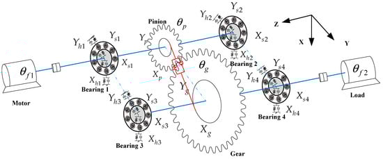
Figure 1.
The 24-DOF coupled model.
To simplify the problem and prioritize the analysis of key variables, the coupled dynamic model focuses on the primary factors while disregarding some secondary factors [27].
- For bearings and gears, only the dynamics in X, Y, and the rotation are taken into consideration;
- The components of the gears and bearings are elastically deformed and satisfy the Hertz contact theory;
- The bending deformation of the shaft in the coupled model is ignored;
- The influence of lubrication and temperature is not considered;
- The sliding between the bearing race and balls is ignored, and only pure rolling is considered.
The coupled dynamics is modeled by the following equations.
Bearing:
Gear:
Shaft:
The 24-DOF dynamic model is established by Equations (1)–(12). In the model, and represent the mass of the pinion and the gear. represent the displacement, velocity, and acceleration of the pinion and the gear in the X-direction. represent the displacement, velocity, and acceleration of the pinion (p) and the gear (g) in the Y-direction. represent the angular displacement, angular velocity, and angular acceleration of the pinion (p) and the gear (g). means the moment of inertia. means the radius of the base circle. Additionally, represent the components of the dynamic normal mesh force among the gear pair. For bearings, represents the mass of the components. represent the supporting damping and supporting stiffness of bearing raceways and represent the contact force. In addition, and represent the displacement, velocity, and acceleration of the bearing. The subscript i = s, h represents the inner race and outer race, and the subscript j = 1, 2, 3, 4 represents the number of bearings, respectively. represent the angular displacement, angular velocity, and angular acceleration of the motor and the load. means the moment of inertia of the load and the motor. represents the torque of the motor and the load.
Considering the meshing between the pinion and the gear, are calculated as follows:
where represents the pressure angle of the gears. The schematic of mesh force is shown in Figure 2.
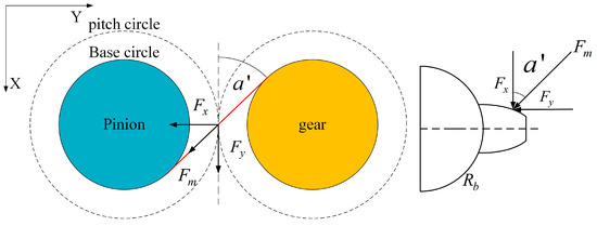
Figure 2.
Decomposition of meshing force.
2.2. Gear-Meshing Force and TVMS
The gear-meshing force is calculated by gear deformation, TVMS, and damping. The calculation of meshing force is provided in Equation (15) [25]:
where represents TVMS and represents mesh damping. The relative displacements and velocities in Equation (15) can be calculated from Equations (16) and (17).
where means the pressure angle and means the base diameter.
It has been established through prior research that gears undergo a range of deformation processes, including shear deformation, bending deformation, radial compression deformation, and Hertzian contact deformation during the meshing process, the subscripts for which are “s”, “b”, “a”, and “h”. The calculation of deformation energy , , and can be conducted using Equations (18)–(20) [28].
In the above equation, represents elastic modulus and is Poisson’s ratio. , , and represent the shear modulus, the cross-sectional area, and the moment of inertia, which can be calculated by Equations (21)–(23):
where represents the width of the gear pair and represents half of the gear thickness.
The shear stiffness , the bending stiffness , the radial compression stiffness , and the deflection stiffness can be calculated by Equations (24)–(27) [29]:
where means the angular displacement that gears go through from the initial position, and and are the limit angular values of tooth pair engagement.
From Hertz’s theory, it is known that can be calculated by Equation (28):
where represents Hertz’s contact stiffness. The TVMS can be calculated by Equation (29):
2.3. Bearing Contact Forces
In the coupling model, the contact relationship of the bearing is calculated by Equation (30) [30]. The deformation and velocity of the bearing between balls and raceways can be calculated by Equations (31) and (32) [31]:
where is the total comprehensive stiffness, is the equivalent damping coefficient, represents the number of rollers, is 1.5 for a ball bearing, represents the ball position, and c represents clearance of the bearing.
The angular position of each ball is calculated by the speed of the bearing inner race. Neglecting the effect of friction, the bearing is not transmitting torsional motion. Therefore, the angular displacement, angular velocity, and angular acceleration of bearings is assumed to be consistent with the input shaft and output shaft in the model. The angular position of balls is calculated as follows:
where is the angular velocity of the cage and is the speed of the inner race, which is consistent with , . represents the outer diameter and represents the pitch diameter. In addition, is the previous ball position.
The and can be obtained through [32]:
where represents the damping radio and represents the mass of each ball. Additionally, represents the Hertz contact stiffness between raceways and balls, which can be calculated by [33]:
where is the curvature sum and is the dimensionless contact deflection.
2.4. Model of Bearing with Defect
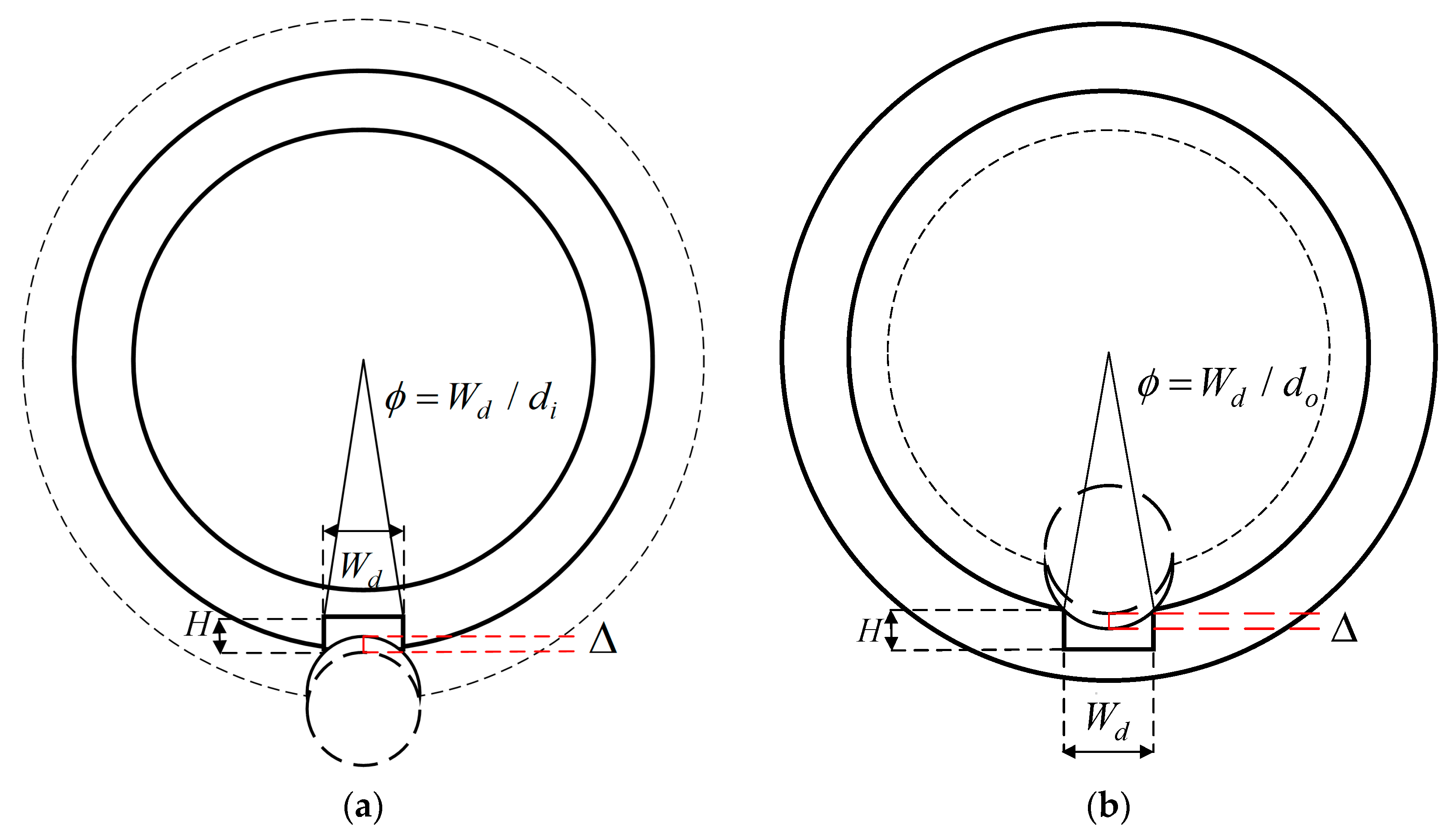
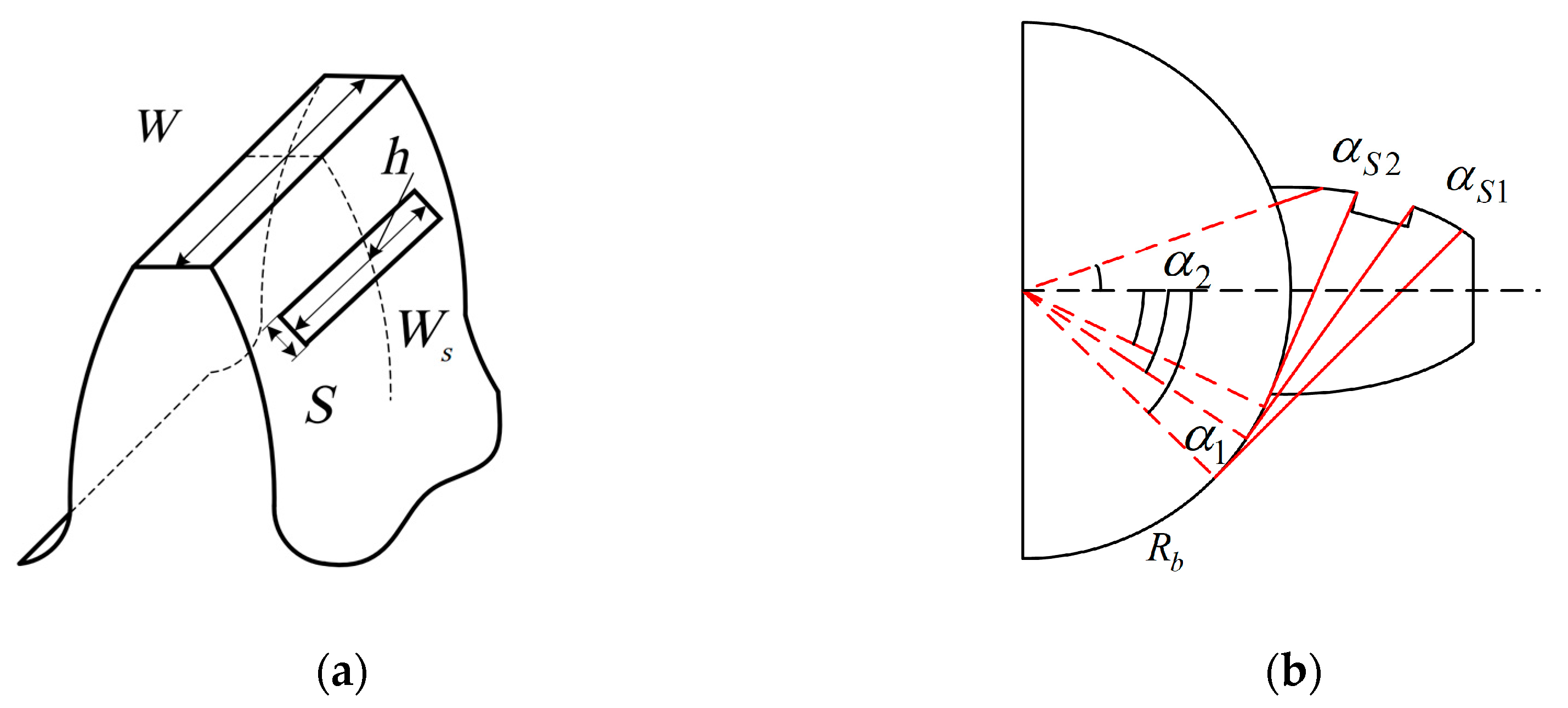
In this article, the geometry of the bearing defect is approximated as a rectangle in order to facilitate the modeling of defect dynamics. The different location of the localized defect is taken into consideration. When the ball passes through the fault, an additional deflection will occur. The schematic diagram of faults on raceways is shown in Figure 3, where is the defect depth and represents the defect width. In addition, and represent the diameters of the raceways.

Figure 3.
Additional defection of the ball due to the fault. (a) Defect on the inner race. (b) Defect on the outer race.
The additional defection of the ball when passing through faults can be calculated by Equation (38). Therefore, the deformation is amended by Equation (39) [34].
Whether the ball enters the defect location is determined by , which is calculated by Equation (33). The conditions for determining whether the ball passes the defect region are different in the coupled model due to the difference in the location of the defect. When the fault is located on the outer race, the raceway is fixed in the housing. Therefore, whether the ball enters the defect location can calculated by Equation (40), where represents the fault position.
When the defect occurs on the inner race, it will rotate with the shaft. And whether the ball enters the defect location can be determined by Equation (41), where represents the angular velocity of the shaft.
2.5. Parameters of Coupled Model
The parameters of gears in coupled model are given in Table 1. The bearings of the coupled model on the two shafts are 6304 and 6207, respectively. The parameters of the bearings are given in Table 2 and Table 3. The characteristic frequencies of the model are shown in Table 4, and the parameters of the defect are shown in Table 5. Other parameters of the model are given in Table 6.

Table 1.
The main parameters of the gear pair.
Table 2.
Main geometry parameters of deep-groove ball bearing 6304.
Table 3.
Main geometry parameters of deep-groove ball bearing 6207.
Table 4.
Characteristic frequencies of the model.
Table 5.
Parameters of the defect.
Table 6.
Parameters of the coupled model.
The gear-meshing frequency (GMF), ball pass frequency on the outer race (BPFO), and ball pass frequency on the inner race (BPFI) of the coupled model are given in Table 4.
In the coupled model, the defects are set on bearing 6304, and the parameters of the defect are given in Table 5.
3. Results
The coupled model is simulated in normal conditions and fault conditions. Due to the established model, as shown in Equations (1)–(12), it consists of ordinary differential equations. Therefore, the coupled model is solved by the Runge–Kutta method in MATLAB 2022a with the variable-order method ode15s. The simulation results are as follows. Additionally, narrowband between 1500 Hz and 2000 Hz is used to envelope.
3.1. Defect on Outer Race
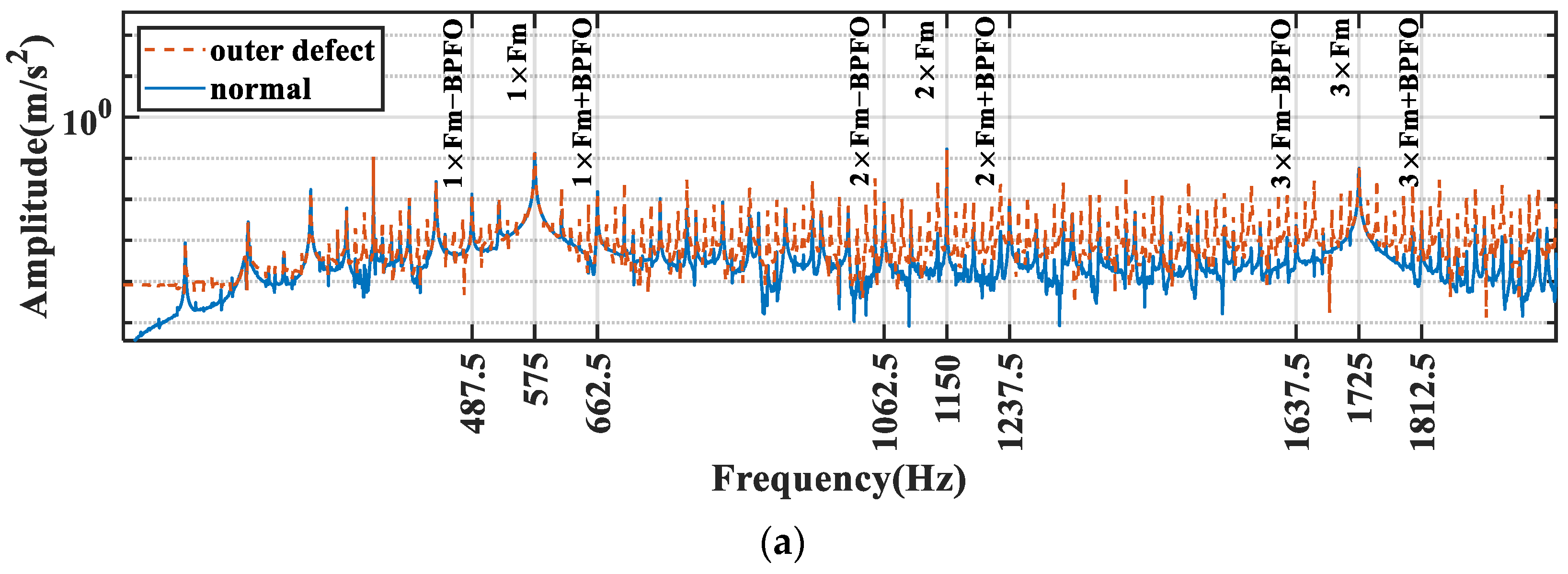
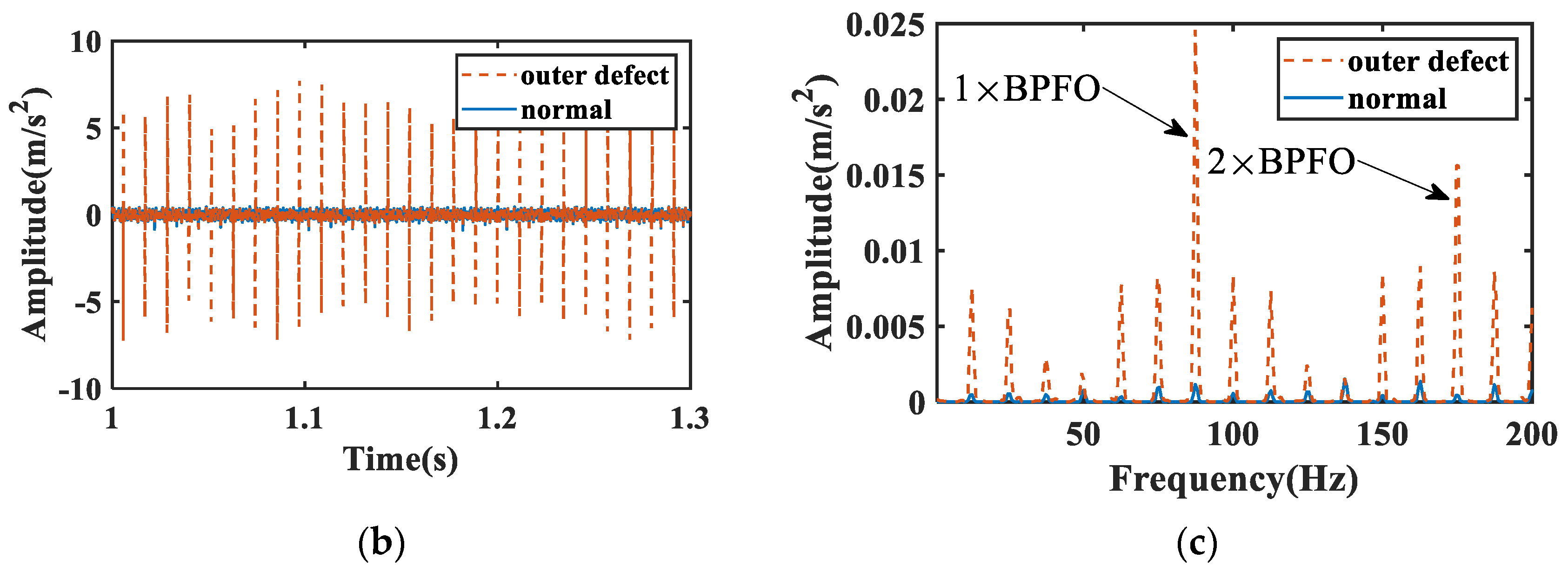
The vibration response analysis when the fault occurs on the outer race is given in Figure 4. From the frequency-domain perspective in Figure 4a, it can also be found that the components of sidebands near GMF are mainly BPFO, and it is mainly due to the fault on the outer race. Correspondingly in Figure 4b, it is obvious that the acceleration waveform produces periodic shocks when the defect occurs on the outer race. And the cycle of shock is the inverse of BPFO. The modulation components are analyzed by the envelope, which is shown in Figure 4c. The difference in amplitudes between normal and outer defects can be found obviously. In addition, the BPFO is obvious.
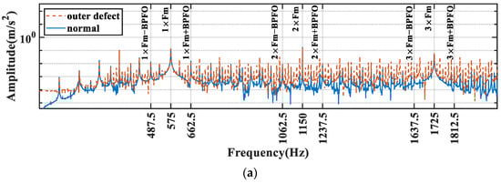
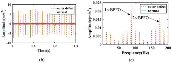
Figure 4.
The acceleration signal of a fault on the outer race of bearing 6304. (a) Acceleration frequency-domain signal. (b) Acceleration time-domain signal. (c) Envelope spectrum of acceleration.
3.2. Defect on Inner Race
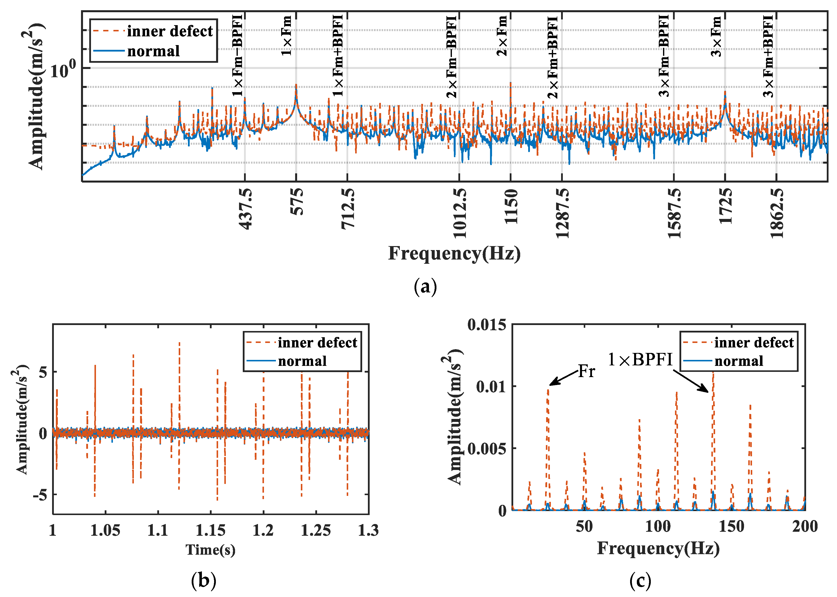
The frequency of acceleration can be seen in Figure 5a. It is obvious that sidebands with modulation-frequency BPFI exist near each GMF. Time-domain waveforms of acceleration are given in Figure 5b, and the acceleration also produces a periodic shock when a defect fault occurs on the inner race. By observing the components of the envelope spectrum in Figure 5c, it is obvious that the modulation components consist of BPFI. In addition, the amplitude of Fr is also easy to find when the defect is located on the inner race of the bearing. This is because the race rotates with the shaft, which affects the cycle time of the ball through the defective area. A rotating shaft and rolling balls together affect the mechanisms of the fault, which is different from the condition when it occurs on the outer race.
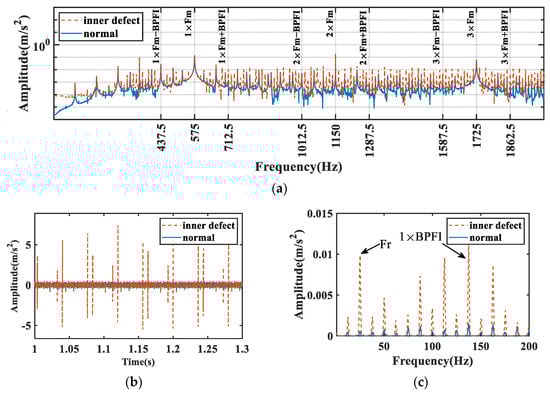
Figure 5.
The acceleration signal of a fault on the inner race of bearing 6304. (a) Acceleration frequency-domain signal. (b) Acceleration time-domain signal. (c) Envelope spectrum of acceleration.
3.3. Numerical Analysis of Defect with Different Size
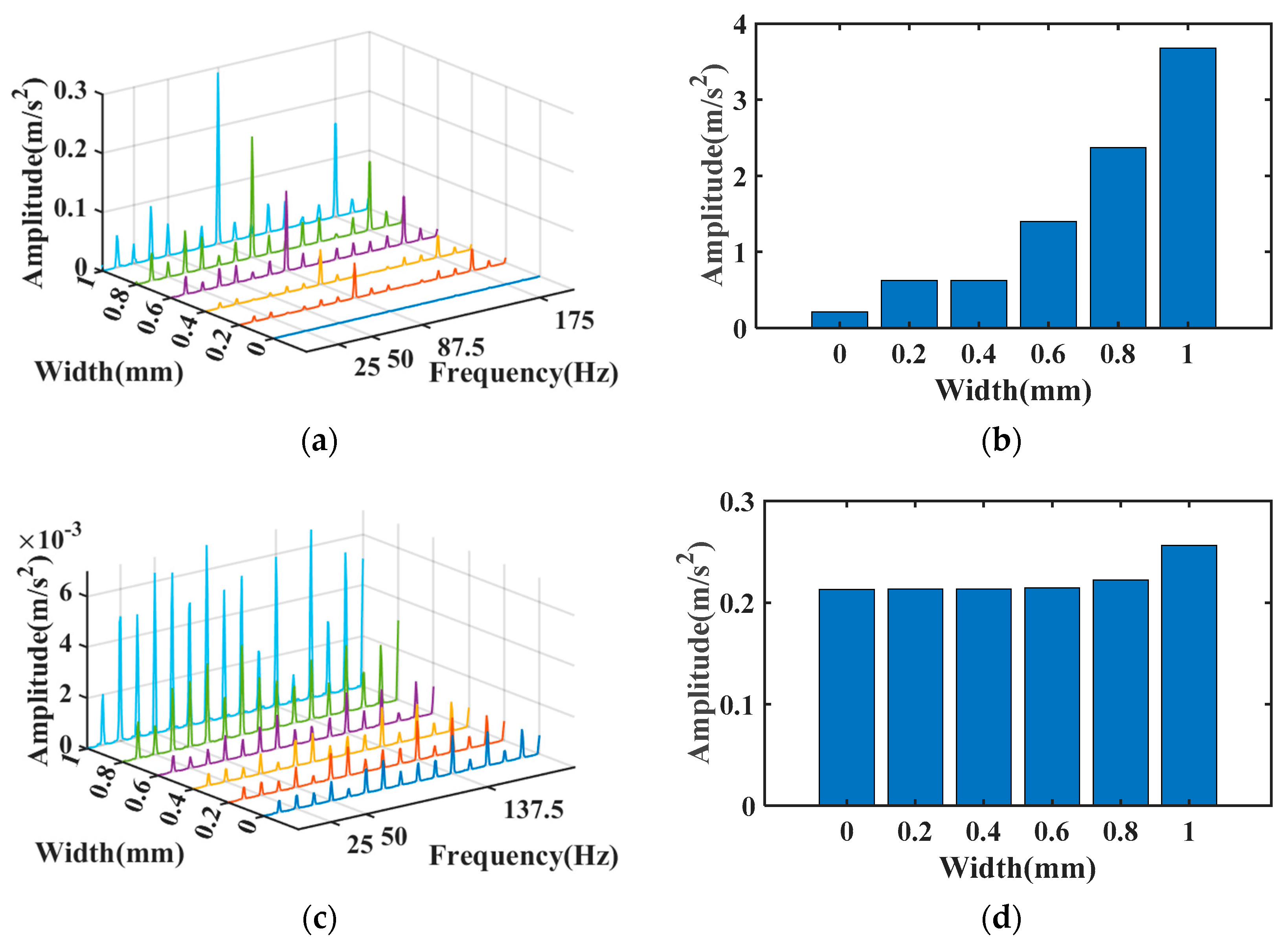
The defect widths are set from 0.2 mm to 1 mm, and the envelope components and RMS are analyzed.
The envelope components and RMS are given in Figure 6, where (a) and (b) represent the envelope spectrum and RMS of acceleration when the defect is on the outer race. The different colors represent envelopes at different loads. It can be found that the envelope amplitude is more obvious with increasing width. The bearing with a localized defect has higher amplitudes of BPFO, which increase with width. Figure 6c,d show the envelope spectrum and RMS of acceleration when the defect is positioned at the inner race. By observing Figure 6d, the amplitudes of Fr and BPFI will both increase with the widening of width. It means the rotation of the inner race and defects both have an influence on the coupled system, which complicates the diagnosis of faults. However, the increase in RMS is not significant when the width is less than 0.6 mm, and this means the diagnosis of small inner-race defects is difficult by calculating the RMS.
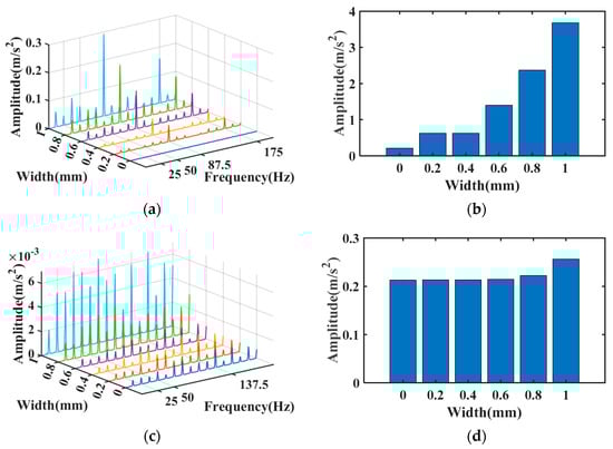
Figure 6.
The vibration characteristics of a defect on the outer race and inner race with different widths. Outer race: (a) Envelope spectrum of acceleration. (b) RMS of acceleration. Inner race: (c) Envelope spectrum of acceleration. (d) RMS of acceleration.
3.4. Numerical Analysis Under Different Loads and Speeds
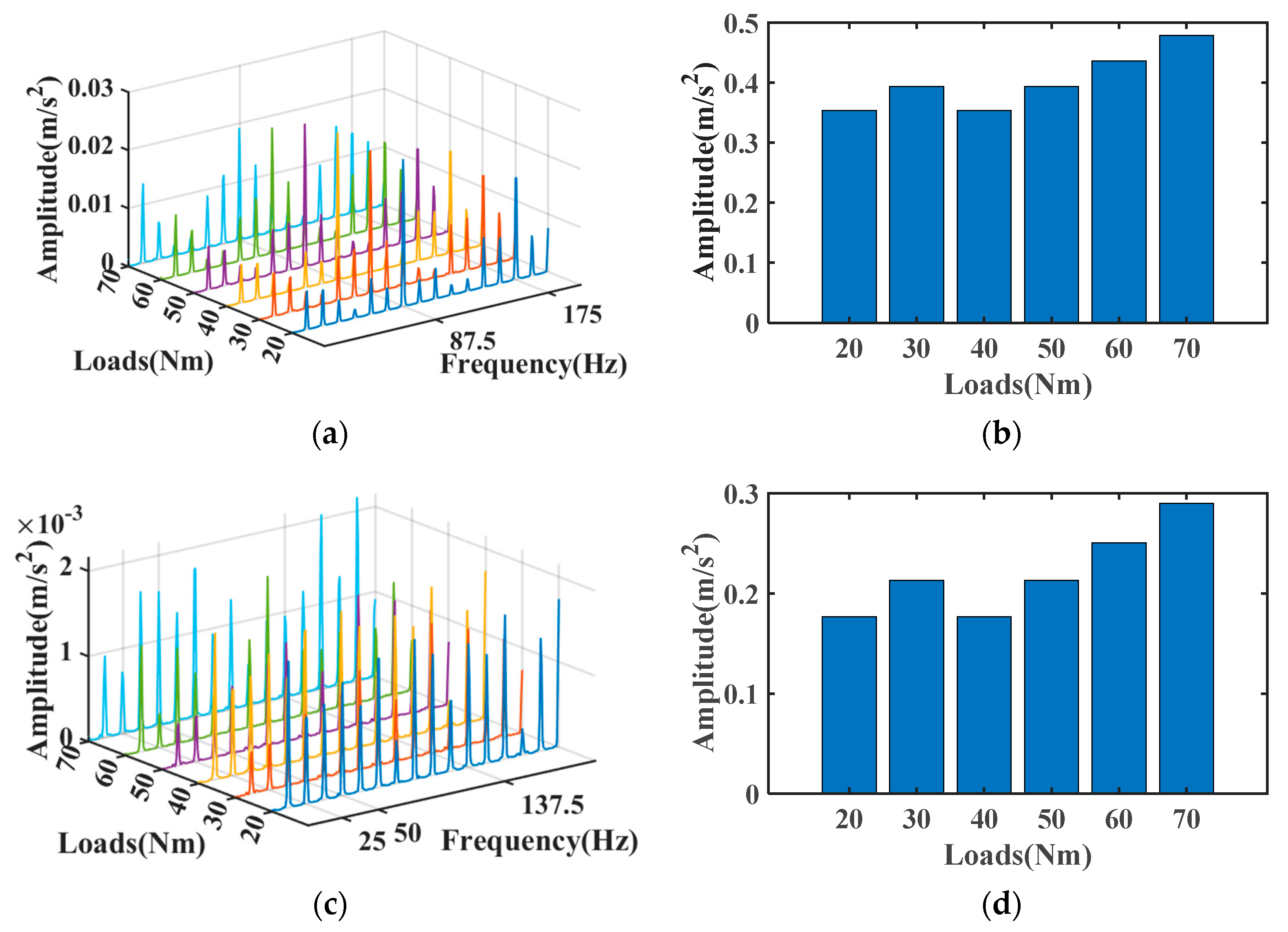
To verify the robustness of the model, simulation under different loads and speeds is carried out. The envelope spectra and RMS of simulation under different loads are shown in Figure 7. The load is set from 20 Nm to 70 Nm.
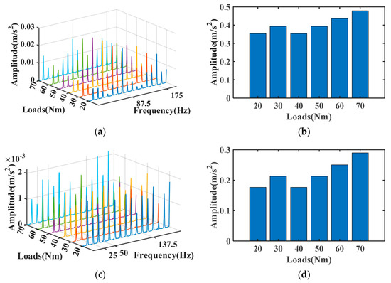
Figure 7.
The vibration characteristics of defect on the outer race and inner race with different loads. Outer race: (a) Envelope spectrum of acceleration. (b) RMS of acceleration. Inner race: (c) Envelope spectrum of acceleration. (d) RMS of acceleration.
Figure 7 shows that the RMS increases with loads in general. The modulation frequencies of the defective bearing, such as BPFI and BPFO, can be clearly detected from envelope spectra under different loads, and the amplitude of these frequencies shows an increase with load, which can verify the robustness of the model under varying load conditions.
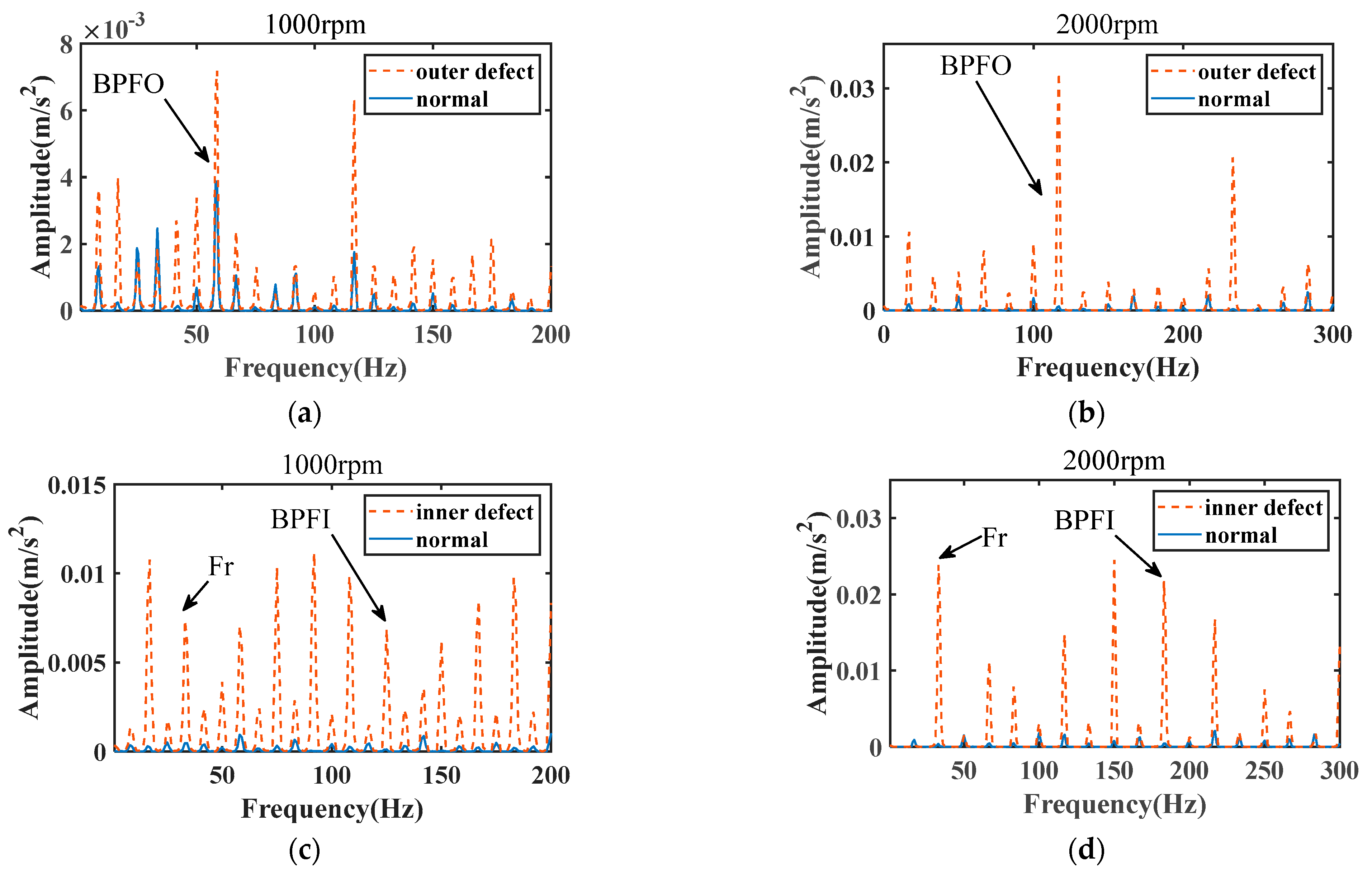
In addition, the simulation under varying speeds is shown in Figure 8. The speed is set up from 1000 rpm to 2000 rpm.
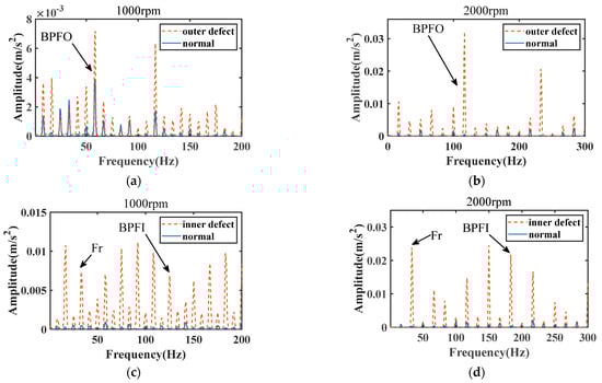
Figure 8.
Envelope spectrum of acceleration: (a,b) outer race; (c,d) inner race.
The values of BPFO at the speeds of 1000 rpm and 2000 rpm are 58.3 Hz and 116.6 Hz. The values of BPFI are 91.6 Hz and 183.3 Hz. Additionally, the values of Fr are 16.7 Hz and 33.3 Hz.
It can be observed that the characteristic frequencies such as BPFO, BPFI, and Fr are consistent with theoretical values. Additionally, the amplitudes of these frequencies show an increase with rotational speed, which validates the robustness of the model at varying speeds.
3.5. Numerical Analysis of Complex Defect on Bearing and Gear
From previous studies, the amplitude of Fr in sideband components increases when an inner-race defect occurs [35]. However, the diagnosis of gear local defects, such as spalling, is also achieved by the detection of shaft frequency components. Consequently, the analysis of the vibration characteristics of the established model with bearing inner-race defects and gear local defects is essential. It is known that early diagnosis of faults is very important, so the defect width is set at 0.2 mm, which simulates the occurrence of early bearing inner-race defects. The graph of the spalling fault can be seen in Figure 9.
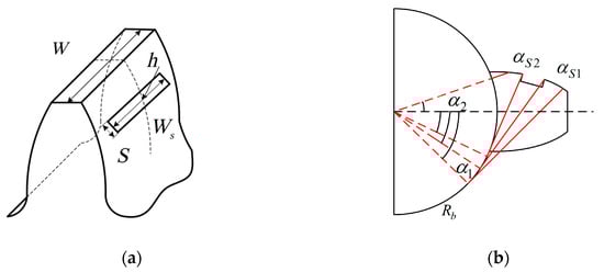
Figure 9.
(a) Schematic diagram of spalling defect. (b) Cantilever beam model of spalling.
Spalling defects in gears can have an effect on the TVMS, so the formula for calculating TVMS when passing the defective region needs to be revised. The angle is used to determine whether the tooth has a spalling fault. The angular range of each tooth is calculated as follows:
where represents the teeth number of the pinion. In the simulation processing, the currently meshed tooth is calculated by and . The number of the spalling tooth is assumed to be the ith; when the tooth corresponding to is the ith tooth, the gear fault is taken into consideration, and the mesh stiffness is calculated according to the spalling stiffness equation.
The shear stiffness, bending stiffness, and axial compression stiffness of a tooth pair entering a defective region can be calculated from the following equations:
where represents the radius of the base circle; and represent the angles of the gear when the pair enters and passes through the spalling region, and they are determined by the defect length . In addition, , , and are given in Table 7.
Table 7.
Parameters of spalling.
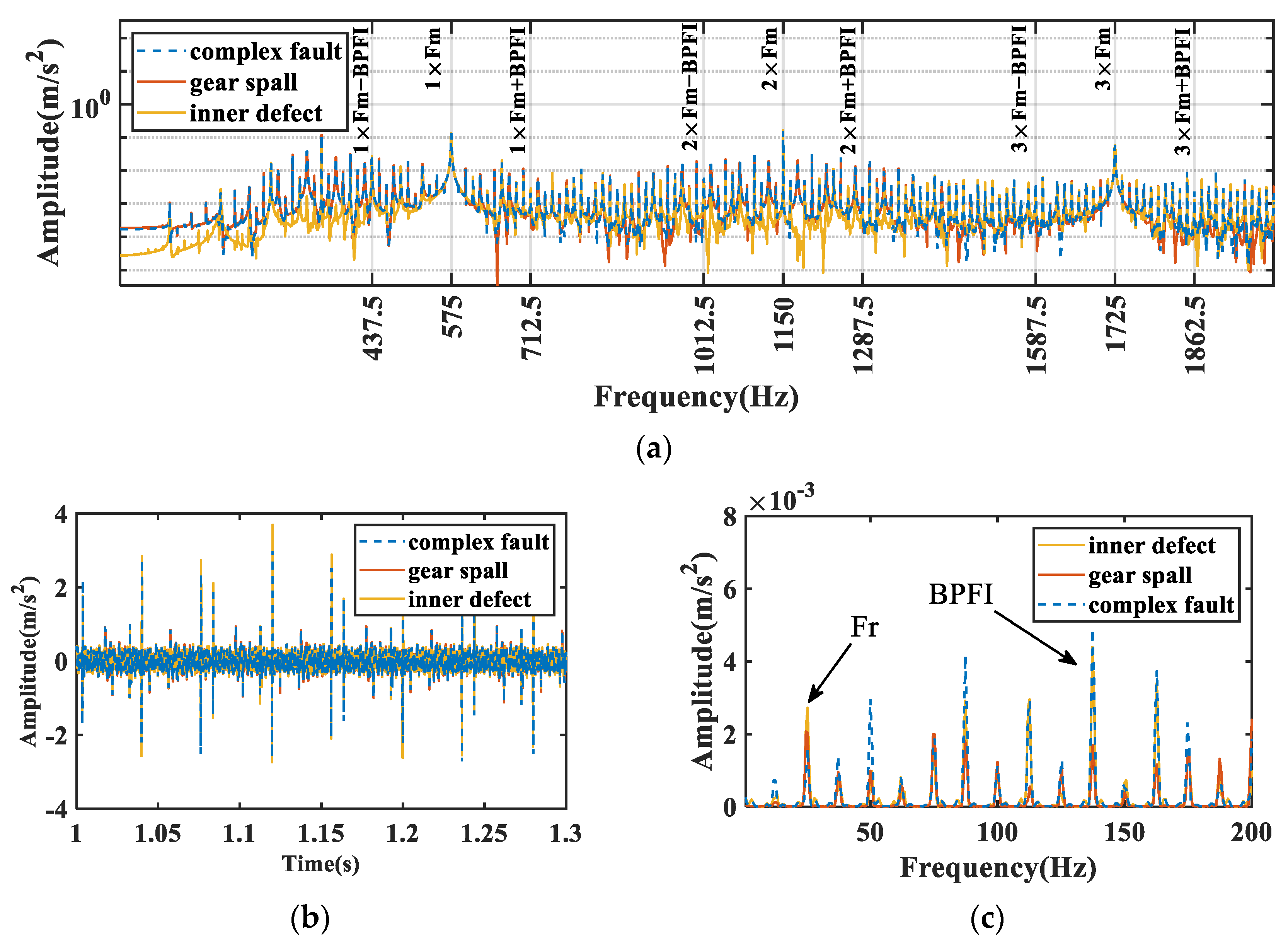
Figure 10 shows the comparison of the vibration characteristics between complex faults and only a single fault. It can be found that the complex defects have more shocks and richer sideband components from Figure 10a, and different faults exhibit variations in both the frequency and amplitude of sideband frequencies. In addition, different time-domain shocks can be found for bearing defects and gear spalling faults. By the envelope which is analyzed, the amplitude of BPFI increases but the amplitude of Fr reduces for models with complex faults, which may be because of the nonlinear coupling relationship of gear and bearing complex faults.
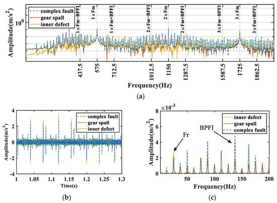
Figure 10.
The vibration characteristics of a system with a complex fault and only inner defects. (a) Acceleration frequency-domain signal. (b) Acceleration time-domain signal. (c) Envelope spectrum of acceleration.
From the above findings, the modulation components of systems with inner-race defects and gear spalling faults are similar. The system has both BPFI and axial-frequency components, differing only in amplitude. This leads to difficulties in diagnosing faults by detecting the modulation components. Especially when complex faults occur in the system at the same time, bearing inner-race defects or gear spall faults may be confused and thus misdiagnosed.
4. Experimental Verification
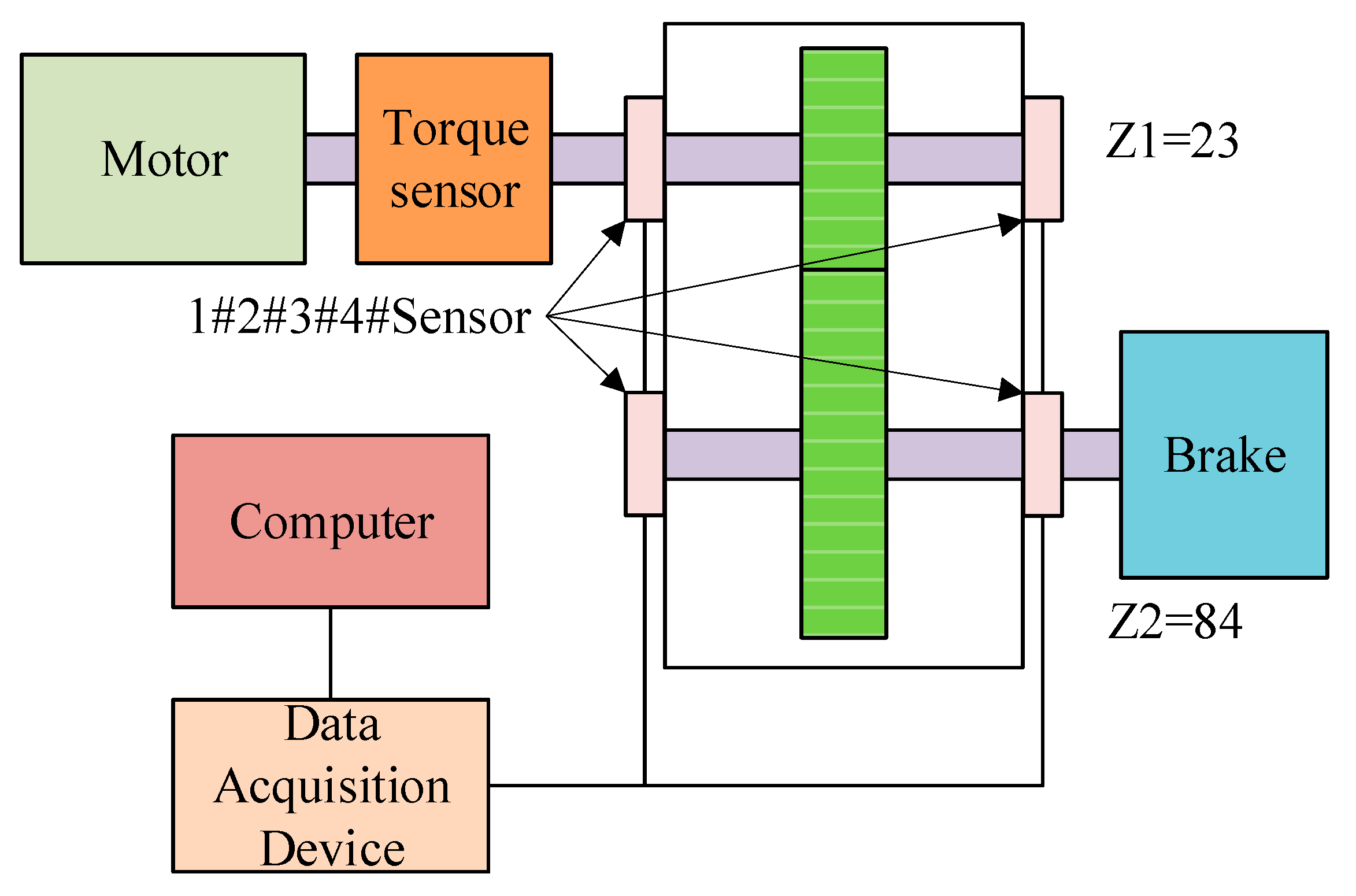
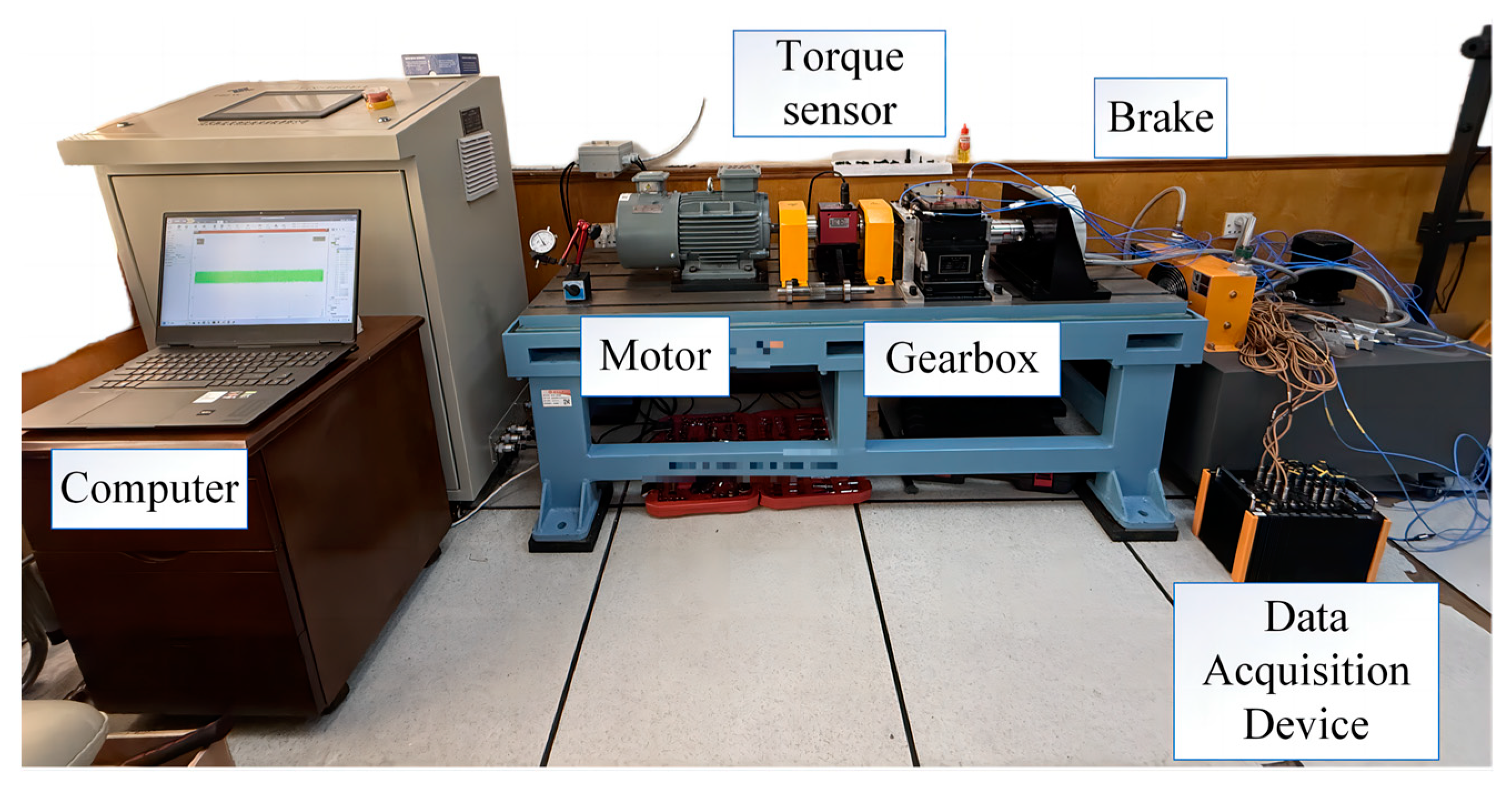
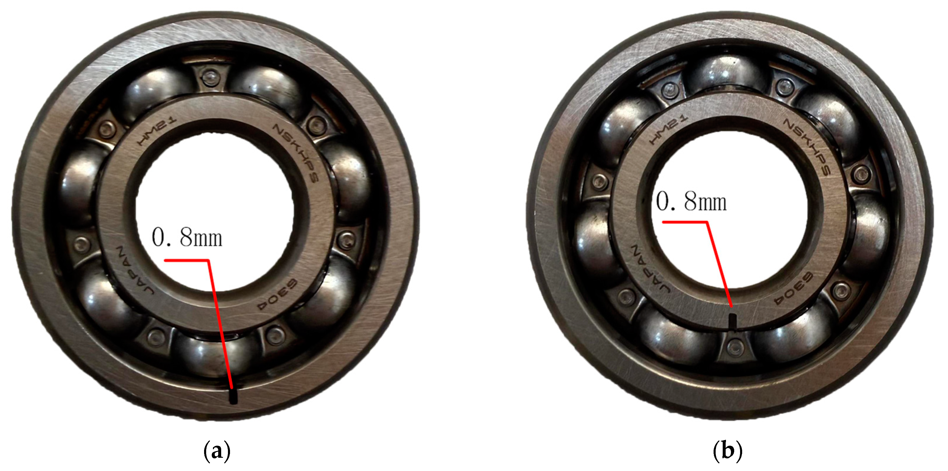
Experiments are designed to verify the established coupled model. The schematic layout of the experimental equipment is given in Figure 11. Additionally, the arrangement of experimental equipment is shown in Figure 12. Sensors #1–#4 are set on the bearing housing. Gearbox experiments are conducted and vibration acceleration signals are collected for bearings with defects, respectively. The defect of the bearing is shown in Figure 13. The widths of defects are set to 0.8 mm. The motor speed is set at 1500 rpm. A magnetic powder brake provides the torque, which is set at 20 Nm.
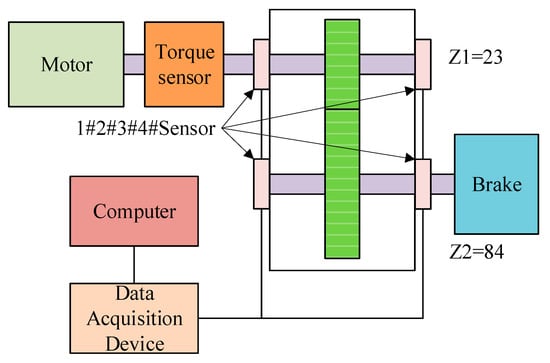
Figure 11.
Schematic layout of experimental equipment.

Figure 12.
Arrangement of experimental equipment.
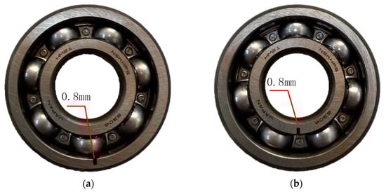
Figure 13.
The defect of bearing. (a) Defect on the outer race. (b) Defect on the inner race.
4.1. Experimental Verification of Defect on Outer Race
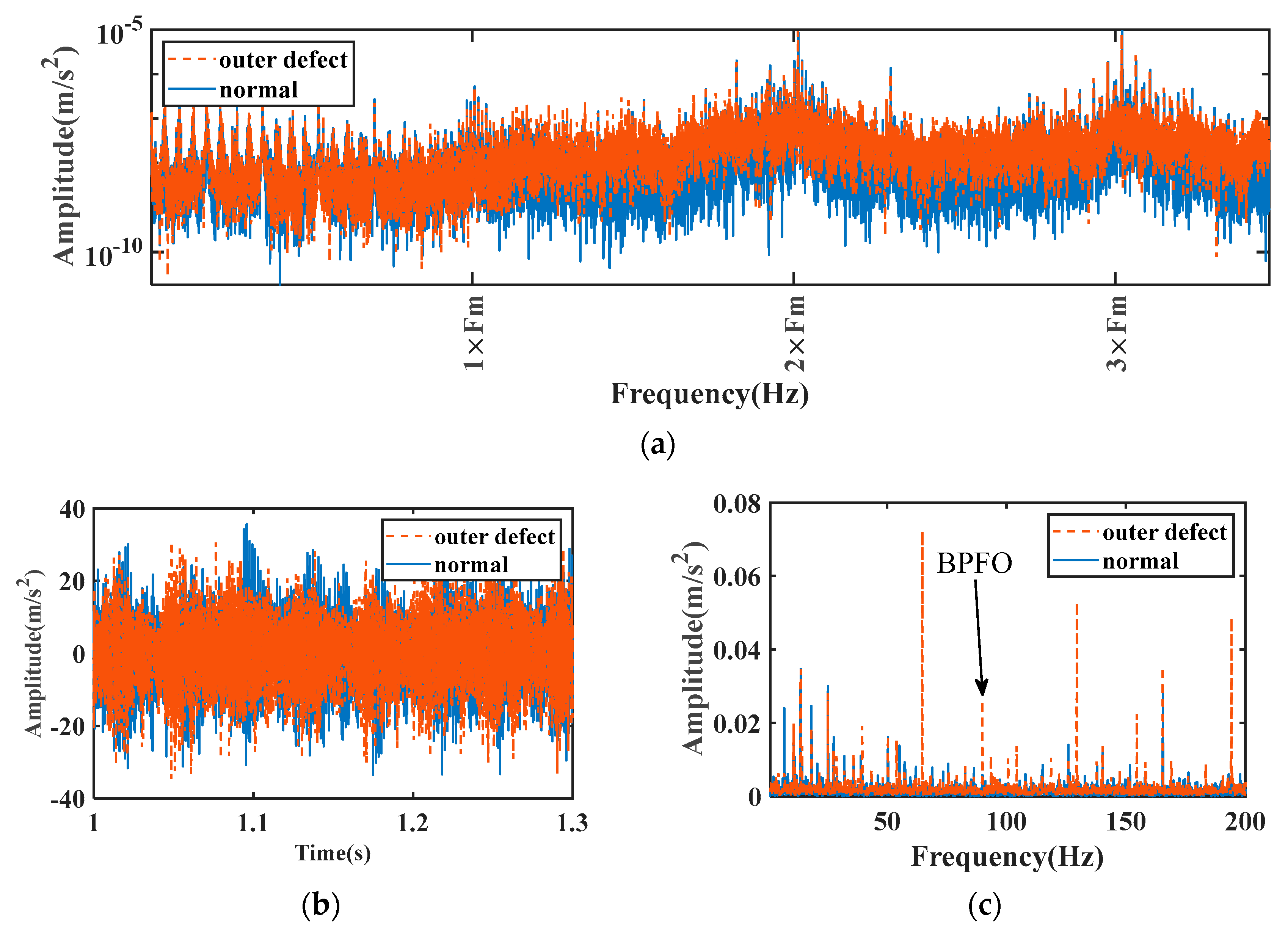
Signals are acquired and analyzed, which are shown in Figure 14. The frequency-domain analysis can be seen in Figure 14a, and time-domain waveforms are displayed in Figure 14b. There are richer sidebands in the frequency spectrum of the bearing with a defect on the outer race. Correspondingly, the time-domain image shows periodic shocks. The sidebands are analyzed by envelope demodulation, which is shown in Figure 14c. The modulation component of BPFO can be detected in Figure 14c, which is due to the defect which is located on the outer race. The high amplitude of the shaft rotation frequency may be due to the misalignment of the shaft.
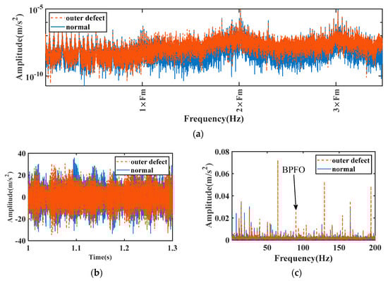
Figure 14.
The vibration characteristics of a defect on the outer race. (a) Acceleration frequency-domain signal. (b) Acceleration time-domain signal. (c) Envelope spectrum of acceleration.
4.2. Experimental Verification of Defect on Inner Race
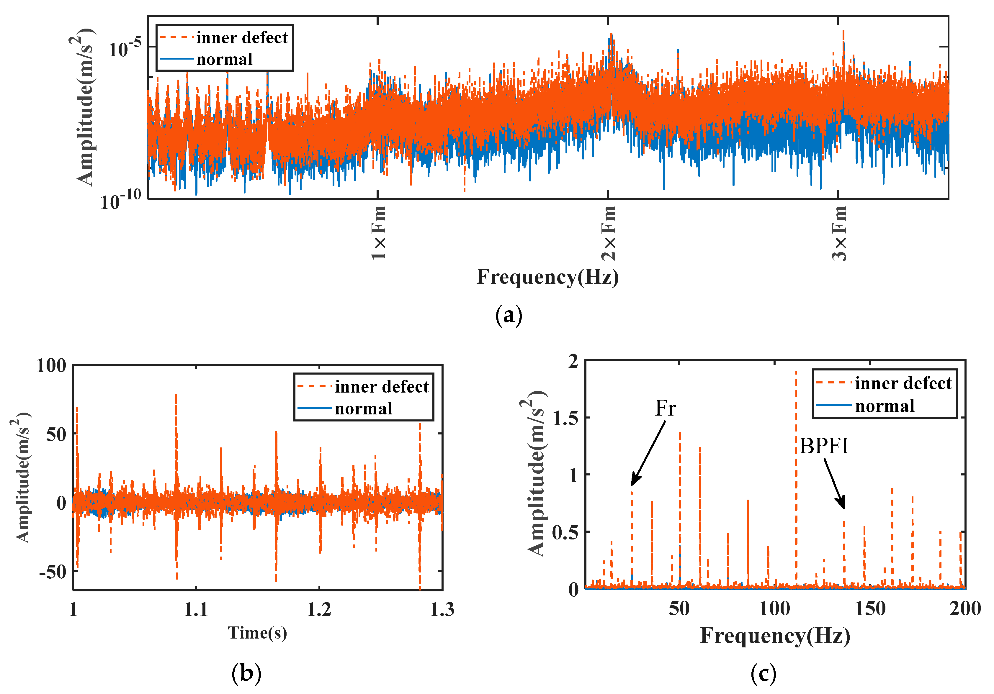
The signals of the bearing when a defect occurs on the inner race are also acquired and analyzed. The acceleration frequency-domain signal is analyzed in Figure 15a, and the time-domain waveforms of the acceleration signal are analyzed in Figure 15b. In addition, acceleration is analyzed by the envelope, which can be seen in Figure 15c. When a defect occurs in the bearing, which is located on the inner raceway, the time-domain signal produces periodic shocks, which will generate more side frequency components in the spectrum, and envelope demodulation is performed for the side frequency components. From Figure 15c, it can be found that when the inner race is defective, the amplitude of each order of the Fr is much larger than that of a normal bearing. In addition, BPFI was also found in the modulation components of inner-ring defective bearings.
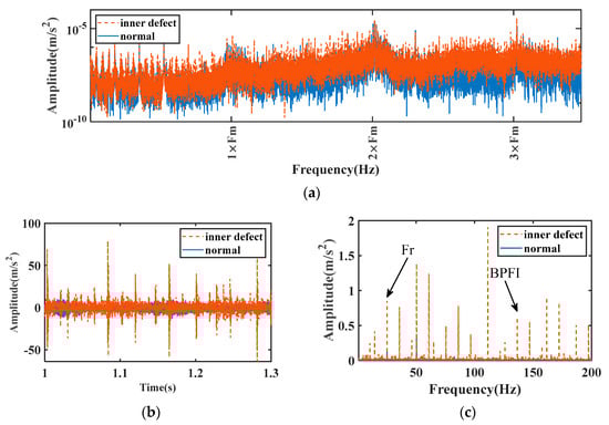
Figure 15.
The vibration characteristics of a defect on the inner race. (a) Acceleration frequency-domain signal. (b) Acceleration time-domain signal. (c) Envelope spectrum of acceleration.
The difference between the simulation and experiment can be seen from the results. The reasons for the difference can be attributed to various factors, such as lubrication, temperature, background noise, and fluctuations in rotational speed and load. Especially, due to the influence of assembly, the shaft of the gearbox and the torque meter are connected by a joint which influences the motion of the shaft in the gearbox. For a bearing with defects, the contact between the rolling balls and the defect are influenced by the joint, which reduces the expected impulse shock due to the defect. Therefore, in the experimental results, the amplitude of BPFO and BPFI are affected by these reasons and they are not as significant as simulation. However, the BPFO, BPFI, and Fr can be detected in the envelope spectra, which match the simulation results in frequency. Therefore, the results initially prove the accuracy and rationality of the simulation model.
5. Discussion
The dynamic model proposed in this paper can simulate the vibration signals of a parallel-axis gearbox with deep-groove ball bearings. And it considers the coupling of bearings and gears, simulating the modulation effect of bearing local fault signals on gear meshing. In addition, the model can simulate the signal of complex faults, including bearing localized defects and gear spalling. In terms of application, the model can serve as a reference for modeling methods in the dynamic simulation of the gear transmission system and provide training data for fault diagnosis models based on machine learning. It can provide characteristic samples with different defects for model training and solve the problem of difficulty in obtaining samples. Additionally, the defect types and defect characteristics are automatically matched, and the parameters of the gearbox and defects can be obtained from the model settings. This makes the labeling of samples more convenient and reduces labor costs.
In future works, based on this research, more complex conditions could be further incorporated, such as waviness characterization, bearing slip effects, and lubrication. In addition, through more accurate modeling, it can simulate the gear transmission system and provide richer and more comprehensive simulation data for fault diagnosis.
6. Conclusions
In this study, a 24-DOF dynamic coupling model is proposed for a parallel-axis gearbox with deep-groove ball bearings, which can be used to simulate the vibrations when localized defects occur in gearboxes. In addition, the vibration of the established model is analyzed. Diagnostic characteristics between bearing internal raceway defects and gear spalling faults are compared and studied. At last, gearbox tests are designed to verify this model.
The proposed model considers the coupling effect of the gear, shaft, and bearings with more DOFs, which makes up for the shortcomings of the previous dynamic model for a gear transmission system. When an outer-race defect occurs in a bearing, the model generates periodic shocks and produces sidebands around frequency peaks, and the modulation frequency of BPFO can be clearly detected through envelope analysis. When an inner-race defect occurs, it also generates periodic shocks and produces sidebands around frequency peaks, and the modulation frequency of BPFI is obvious, as well as the amplitude of the shaft frequency. Through simulation, for a localized defect on bearing raceways, when the defect size increases, the amplitude of BPFI and BPFO will increase, but this increase is nonlinear. When a local defect appears on the bearing inner race and gear surface, the amplitude of the shaft frequency increases and there is a similarity in the sidebands and components of the envelope—which increases the difficulty in identifying the frequency of failures of bearings and gears. This result provides optimization directions for subsequent fault diagnosis methods for distinguishing between spalled gears and bearing inner-ring defects by detecting Fr. Experiments considering bearing defects are designed. The experiments show similar results with simulation when defects are located on raceways. Gearbox tests validate the accuracy of the model, which can be used to simulate bearing failures in further research.
The proposed dynamic model can provide a theoretical foundation and sufficient samples for accurate diagnosis of the gear transmission system, which is meaningful for condition monitoring and the maintenance of the gearbox.
Author Contributions
Conceptualization, M.X.; methodology, Y.Z. and Y.H.; software, Y.Z.; validation, Y.Z., J.Z. and D.Q.; investigation, Y.Z. and Y.H.; formal analysis, Y.Z., J.Z. and D.Q.; writing—original draft preparation, Y.Z.; writing—review and editing, Y.Z., Y.H., W.H. and M.X.; supervision, W.H. and M.X.; funding acquisition, W.H. and M.X. All authors have read and agreed to the published version of the manuscript.
Funding
This research was supported by Guangxi Natural Science Foundation (Grant Nos. 2024GXNSFBA010142, 2025GXNSFAA069184), the Project for Enhancing Young and Middle-aged Teachers’ Research Basis Ability in the Colleges of Guangxi (Grant No. 2024KY0013), and Guangxi Science and Technology Major Program (Grant Nos. AA24206039, AA23062001), China.
Data Availability Statement
The original contributions presented in this study are included in the article. Further inquiries can be directed to the corresponding authors.
Conflicts of Interest
The authors declare no conflicts of interest.
Abbreviations
The following abbreviations are used in this manuscript:
| RB | Roller bearing |
| LOD | Localized defect |
| DOF | Degree of freedom |
| BPFO | Ball pass frequency on outer race |
| BPFI | Ball pass frequency on inner race |
| GMF | Gear-meshing frequency |
| Fr | Rotation frequency |
| TVMS | Time-varying meshing stiffness |
References
- Matania, O.; Bachar, L.; Khemani, V.; Das, D.; Azarian, M.H.; Bortman, J. One-fault-shot learning for fault severity estimation of gears that addresses differences between simulation and experimental signals and transfer function effects. Adv. Eng. Inform. 2023, 56, 101945. [Google Scholar] [CrossRef]
- Liu, J.; Shao, Y.M.; Lim, T.C. Vibration analysis of ball bearings with a localized defect applying piecewise response function. Mech. Mach. Theory 2012, 56, 156–169. [Google Scholar] [CrossRef]
- Niu, L.K.; Cao, H.R.; He, Z.J.; Li, Y.M. Dynamic Modeling and Vibration Response Simulation for High Speed Rolling Ball Bearings With Localized Surface Defects in Raceways. J. Manuf. Sci. Eng.-Trans. ASME 2014, 136, 041015. [Google Scholar] [CrossRef]
- Liu, J.; Shao, Y.M. A new dynamic model for vibration analysis of a ball bearing due to a localized surface defect considering edge topographies. Nonlinear Dyn. 2015, 79, 1329–1351. [Google Scholar] [CrossRef]
- Zhang, H.; Li, Z.; Liu, H.; Liu, T.; Wang, Q. Modeling and Dynamic Analysis of Double-Row Angular Contact Ball Bearing–Rotor–Disk System. Lubricants 2024, 12, 441. [Google Scholar] [CrossRef]
- Liu, J.; Shao, Y.M.; Zhu, W.D. A New Model for the Relationship Between Vibration Characteristics Caused by the Time-Varying Contact Stiffness of a Deep Groove Ball Bearing and Defect Sizes. J. Tribol.-Trans. Asme 2015, 137, 031101. [Google Scholar] [CrossRef]
- Xi, S.T.; Cao, H.R.; Chen, X.F.; Niu, L.K. Dynamic modeling of machine tool spindle bearing system and model based diagnosis of bearing fault caused by collision. In Proceedings of the 8th CIRP Conference on High Performance Cutting, Budapest, Hungary, 25–27 June 2018; pp. 614–617. [Google Scholar]
- Liu, J.; Shao, Y.M. An improved analytical model for a lubricated roller bearing including a localized defect with different edge shapes. J. Vib. Control 2018, 24, 3894–3907. [Google Scholar] [CrossRef]
- Yan, C.; Kang, J.; Yuan, H.; Wu, L.; Wei, Y. Dynamic modeling for local defect displacement excitation in rolling bearing systems under elasto-hydrodynamic lubrication and slip. J. Vib. Shock 2018, 37, 56–64. [Google Scholar]
- Liu, C.; Zhang, X.; Wang, R.; Guo, Q.; Li, J. Vibration-Based Detection of Axlebox Bearing Considering Inner and Outer Ring Raceway Defects. Lubricants 2024, 12, 142. [Google Scholar] [CrossRef]
- Gao, Q.F.; Wu, X.X.; Li, Z.S. Failure Analysis of Rolling Bearings Based on Explicit Dynamic Method and Theories of Hertzian Contact. J. Fail. Anal. Prev. 2019, 19, 1645–1654. [Google Scholar] [CrossRef]
- Zhao, Z.Q.; Yin, X.B.; Wang, W.Z. Effect of the raceway defects on the nonlinear dynamic behavior of rolling bearing. J. Mech. Sci. Technol. 2019, 33, 2511–2525. [Google Scholar] [CrossRef]
- Zhang, F.L.; Zhang, Y.W.; Guan, J.Y.; Tian, J.; Wang, Y.J. Fault Dynamic Modeling and Characteristic Parameter Simulation of Rolling Bearing with Inner Ring Local Defects. Shock Vib. 2021, 2021, 5077366. [Google Scholar] [CrossRef]
- Liu, J.; Wang, L.F.; Shi, Z.F. Dynamic modelling of the defect extension and appearance in a cylindrical roller bearing. Mech. Syst. Signal Process. 2022, 173, 109040. [Google Scholar] [CrossRef]
- Ruan, D.W.; Chen, Y.X.; Gühmann, C.; Yan, J.P.; Li, Z.R. Dynamics Modeling of Bearing with Defect in Modelica and Application in Direct Transfer Learning from Simulation to Test Bench for Bearing Fault Diagnosis. Electronics 2022, 11, 622. [Google Scholar] [CrossRef]
- Xue, S.; Jin, Z.; Wang, C.S.; Lian, P.Y.; Li, Y.; Xu, Q.; Li, N.; Wang, X.J. The compound fault interaction analysis of the planet bearing system. J. Braz. Soc. Mech. Sci. Eng. 2022, 44, 606. [Google Scholar] [CrossRef]
- Galli, F.; Sircoulomb, V.; Fiore, G.; Hoblos, G.; Weber, P. Dynamic modelling for non-stationary bearing vibration signals. In Proceedings of the 31st Mediterranean Conference on Control and Automation (MED), Limassol, Cyprus, 26–29 June 2023; pp. 49–54. [Google Scholar]
- Sawalhi, N.; Randall, R.B. Simulating gear and bearing interactions in the presence of faults—Part II: Simulation of the vibrations produced by extended bearing faults. Mech. Syst. Signal Process. 2008, 22, 1952–1966. [Google Scholar] [CrossRef]
- Hu, Z.H.; Tang, J.Y.; Zhong, J.; Chen, S.Y.; Yan, H.Y. Effects of tooth profile modification on dynamic responses of a high speed gear-rotor-bearing system. Mech. Syst. Signal Process. 2016, 76–77, 294–318. [Google Scholar] [CrossRef]
- Xiao, H.F.; Zhou, X.J.; Liu, J.; Shao, Y.M. Vibration transmission and energy dissipation through the gear-shaft bearing-housing system subjected to impulse force on gear. Measurement 2017, 102, 64–79. [Google Scholar] [CrossRef]
- Tian, G.; Gao, Z.H.; Liu, P.; Bian, Y.S. Dynamic Modeling and Stability Analysis for a Spur Gear System Considering Gear Backlash and Bearing Clearance. Machines 2022, 10, 439. [Google Scholar] [CrossRef]
- Feng, W.; Wu, L.J.; Liu, Y.X.; Liu, B.G.; Liu, Z.Y.; Zhang, K. Dynamic Analysis of Geared Rotor System with Hybrid Uncertainties. Chin. J. Mech. Eng. 2024, 37, 112. [Google Scholar] [CrossRef]
- Xu, Z.L.; Yu, W.N.; Xu, H.C.; Li, J.J. Dynamic modeling of spur gear system considering the coupling effect between bearing deflection and gear mesh stiffness. Proc. Inst. Mech. Eng. Part C-J. Mech. Eng. Sci. 2024, 238, 6725–6737. [Google Scholar] [CrossRef]
- Li, W.; Tan, Y.L.; Li, Z.Y.; Tao, Y.P. Analysis of Dynamic Features of Gear-Bearing Systems with Bearing Raceway Failures. J. Fail. Anal. Prev. 2023, 23, 2105–2117. [Google Scholar] [CrossRef]
- Xu, H.Y.; Zhao, X.; Ma, H.; Luo, Z.; Han, Q.K.; Wen, B.C. Vibration analysis of a gear-rotor-bearing system with outer-ring spalling and misalignment. J. Cent. South Univ. 2024, 31, 511–525. [Google Scholar] [CrossRef]
- Zhao, W.Q.; Liu, J.; Zhao, W.H.; Zheng, Y. An investigation on vibration features of a gear-bearing system involved pitting faults considering effect of eccentricity and friction. Eng. Fail. Anal. 2022, 131, 105837. [Google Scholar] [CrossRef]
- Xu, H.Y.; Ma, H.; Wen, B.G.; Yang, Y.; Li, X.P.; Luo, Z.; Han, Q.K.; Wen, B.C. Dynamic characteristics of spindle-bearing with tilted pedestal and clearance fit. Int. J. Mech. Sci. 2024, 261, 108683. [Google Scholar] [CrossRef]
- Dai, P.; Wang, J.P.; Yan, S.P.; Jiang, B.C.; Wang, F.T.; Niu, L.K. Effects of Localized Defects of Gear-Shaft-Bearing Coupling System on the Meshing Stiffness of Gear Pairs. J. Vib. Eng. Technol. 2022, 10, 1153–1173. [Google Scholar] [CrossRef]
- Han, Y.Y.; Ding, X.X.; Gu, F.S.; Chen, X.H.; Xu, M.M. Dual-drive RUL prediction of gear transmission systems based on dynamic model and unsupervised domain adaption under zero sample. Reliab. Eng. Syst. Saf. 2025, 253, 110442. [Google Scholar] [CrossRef]
- Xu, M.M.; Miao, D.X.; Gao, Y.; Yang, R.; Gu, F.S.; Shao, Y.M. A bearing dynamic model based on novel Gaussian-filter waviness characterizing method for vibration response analysis. Tribol. Int. 2024, 194, 109433. [Google Scholar] [CrossRef]
- Xu, M.M.; Han, Y.Y.; Sun, X.Q.; Shao, Y.M.; Gu, F.S.; Ball, A.D. Vibration characteristics and condition monitoring of internal radial clearance within a ball bearing in a gear-shaft-bearing system. Mech. Syst. Signal Process. 2022, 165, 108280. [Google Scholar] [CrossRef]
- Xu, M.M.; Wang, M.C.; He, D.; Ding, X.X.; Shao, Y.M.; Gu, F.S. Skidding behavior of lubricated rolling element bearings under the influence of oil film and radial clearances. Tribol. Int. 2024, 194, 109500. [Google Scholar] [CrossRef]
- Xu, M.; Feng, G.; He, Q.; Gu, F.; Ball, A. Vibration Characteristics of Rolling Element Bearings with Different Radial Clearances for Condition Monitoring of Wind Turbine. Appl. Sci. 2020, 10, 4731. [Google Scholar] [CrossRef]
- Niu, L.K.; Cao, H.R.; He, Z.J.; Li, Y.M. A systematic study of ball passing frequencies based on dynamic modeling of rolling ball bearings with localized surface defects. J. Sound Vib. 2015, 357, 207–232. [Google Scholar] [CrossRef]
- Dong, Y.; Liao, M. Dynamic Analysis on Rolling Element Bearings with Localized Defects Part II a Single Defect in Inner Race. Mech. Sci. Technol. 2012, 31, 689–693. [Google Scholar]


Disclaimer/Publisher’s Note: The statements, opinions and data contained in all publications are solely those of the individual author(s) and contributor(s) and not of MDPI and/or the editor(s). MDPI and/or the editor(s) disclaim responsibility for any injury to people or property resulting from any ideas, methods, instructions or products referred to in the content. |
© 2025 by the authors. Licensee MDPI, Basel, Switzerland. This article is an open access article distributed under the terms and conditions of the Creative Commons Attribution (CC BY) license (https://creativecommons.org/licenses/by/4.0/).