Abstract
This paper introduces a multi-indicator heuristic evaluation-based rapidly exploring random tree (MIHE-RRT) algorithm to address the key challenges of robot path planning in complex environments. The core innovation lies in a novel dual optimization framework that combines Hammersley sequence sampling with a comprehensive multi-indicator heuristic evaluation mechanism. The Hammersley sequence ensures uniform coverage of the configuration space, while the multi-indicator heuristic evaluation mechanism intelligently guides tree expansion through a three-dimensional evaluation system incorporating diversity, distance, and angle values. After generating the initial path, a pruning algorithm removes redundant points to produce an efficient and practical final path. Extensive experimental validation in four different environmental scenarios (semi-enclosed, maze, chaotic, and crowded) demonstrates that MIHE-RRT outperforms RRT (rapidly exploring random tree), IBi-RRT (improved bidirectional rapidly exploring random tree), and HB-RRT (halton biased rapidly exploring random tree) algorithms. Results show significant improvements in planning efficiency (54–88% reduction in execution time), path quality (15–24% shorter paths), and computational resource utilization (77–94% reduction in nodes). These excellent performance metrics not only prove MIHE-RRT’s advantages in complex environments but also make it particularly suitable for practical robot navigation applications requiring reliable and efficient path planning.
1. Introduction
With the improvement of automation in various industries, climbing robots are gradually integrated into daily life. With flexibility and adaptability, they can perform tasks in complex environments such as vertical walls and ceilings, showcasing broad prospects in industrial maintenance, building inspection, and hazardous operations. Within this framework, path planning, as a key technology for climbing robots [1], directly affects the robots’ operational efficiency and task quality.
In the development of path planning algorithms, path planning algorithms have been categorized into graph search algorithms [2,3], sampling-based algorithms [4,5], potential field algorithms [6,7], and biomimetic algorithms [8,9]. The robot path planning algorithm needs to solve two problems: computational efficiency and applicability to different scenarios.
The RRT algorithm [10] is renowned for its probabilistic completeness and efficient search capabilities, enabling planning in both high- and low-dimensional spaces through pseudo-random sampling. However, this pseudo-random sampling characteristic brings limitations, specifically manifesting as insufficient search space coverage due to lower randomness, leading to inefficient planning and difficulties in finding effective path planning solutions in complex environments. To overcome these limitations, Karaman et al. [11] proposed the RRT* algorithm, which maintained RRT’s efficient exploration characteristics while gradually optimizing paths. In RRT’s subsequent evolution, Kuffner et al. [12] proposed the RRT-Connect algorithm, which improved map search efficiency, reduced time through dual-tree expansion, and introduced greedy strategies in the auxiliary tree.
To further enhance algorithm performance, researchers have introduced various heuristic strategies. Informed-RRT* [13] generates optimal paths using hyperellipsoid sampling based on non-uniform sampling. CBQ-RRT* [14] considers kinematic constraints, optimizes path smoothness and length, and combines bidirectional expansion to improve efficiency. CAF-RRT* [15] uses a bi-directional RRT algorithm and parent node optimization selection strategy to generate basic paths, then employs arc smoothing and triangle optimization strategies to improve path smoothness and safety. HB-RRT [16] combines heuristic candidate pool strategy and goal-oriented strategy to provide high-quality sampling points. Hybrid-RRT* [17] significantly improves convergence speed and success rate by combining uniform and non-uniform sampling. CCPF-RRT [18] effectively avoids specific congested areas and optimizes movement costs through congestion and path length cost functions. FC-RRT [19] significantly improves path planning initialization speed and optimization efficiency through dual-path tree searching and an improved reconnection process. The IBi-RRT algorithm [20] combines a random node priority selection strategy and an adjustable attraction size strategy to reduce search randomness and avoid excessive exploration in the same area.
However, these heuristic strategies face challenges in complex environments. Although Neural RRT* [21] achieves intelligent guidance of the sampling process by integrating CNN (Convolutional Neural Network), it requires large training datasets and time-consuming preprocessing. While PBG-RRT [22] improves search efficiency through heuristic probability strategy and bias target factor, it has high computational complexity. Although DG-RRT [23] uses gradient ascent distribution to extend paths, it still struggles with the “dead zone” problem in complex obstacle environments. PF-RRT* [24] combines improved artificial potential fields to alleviate local minimum problems and accelerate convergence to some extent, but has high computational overhead. SARRT-RRT [25] improves planning efficiency and quality through structure-aware cost maps and path optimization, but cost map computation is time-consuming.
Although the RRT algorithm and its heuristic variants (such as IBi-RRT, HB-RRT, etc.) have made significant progress in path planning, they face three major challenges in complex environments:
- Sampling efficiency problem: Existing algorithms generally suffer from an uneven distribution of sampling points and insufficient sampling in key areas.
- Balance problem: Difficulty in achieving a good balance between exploration efficiency and path quality.
- Computational resource problem: Many improved methods result in significant increases in computational overhead.
These limitations seriously affect the algorithms’ performance in practical applications, especially in scenarios requiring precise navigation.
To overcome these limitations, this study proposes the MIHE-RRT algorithm, which improves path planning performance through three key innovations:
- Hammersley sequence sampling: The pseudo-random sampling of traditional RRT often leads to the uneven distribution of sampling points, resulting in oversampling in some areas and undersampling in others. This study adopts the Hammersley sequence sampling technique in MIHE-RRT to ensure the uniform distribution of sampling points in the configuration space, effectively avoiding common clustering and sampling blind spots in traditional Monte Carlo sampling and significantly improving spatial exploration efficiency.
- Multi-indicator heuristic evaluation mechanism: This study proposes a comprehensive evaluation system for MIHE-RRT that achieves a dynamic balance between exploration and development by simultaneously considering three dimensions of indicators: diversity value (to avoid duplicate sampling), distance value (to optimize path length), and angle value (to ensure progress towards the goal). This effectively prevents algorithms from over-exploring
- Tree pruning algorithm: This study integrates a specialized tree pruning algorithm into MIHE-RRT to solve the common problems of redundant nodes and unnecessary turns in RRT-generated paths. Our algorithm significantly shortens path length, improves path practicality, and increases execution efficiency by optimizing node distribution and simplifying path structure.
These three key innovations—Hammersley sequence sampling, multi-indicator heuristic evaluation mechanism, and a tree pruning algorithm—form the complete technical framework of the MIHE-RRT algorithm, jointly solving the core challenges faced by traditional RRT algorithms in complex environments. Table 1 compares MIHE-RRT with existing RRT variant algorithms in terms of key technical characteristics.

Table 1.
Comparison of key characteristics between MIHE-RRT and some existing RRT variant algorithms.
As can be seen from the comparison in the table above, the MIHE-RRT algorithm has distinct technical characteristics in terms of sampling method, heuristic strategy, and path optimization.
The structure of this paper is as follows:
Section 2 introduces the principle of the Hammersley sequence, multi-indicator heuristic evaluation, the time complexity of the algorithm, and tree pruning. In Section 3, the MIHE-RRT algorithm and standard RRT, IBi-RRT, and HB-RRT algorithms are simulated and compared to evaluate the performance of the MIHE-RRT algorithm. Section 4 summarizes this paper’s contribution and future research directions.
2. MIHE-RRT
This second part describes the related strategies of MIHE-RRT. Section 2.1 describes the principle of the Hammersley sequence sampling. Section 2.2 describes the principle of the multi-indicator heuristic evaluation mechanism. Section 2.3 describes the path-smoothing method. Section 2.4 describes the time complexity of the algorithm.
Unlike existing RRT variants, MIHE-RRT proposes a novel dual-layer optimization framework that organically combines Hammersley sequence sampling with the multi-indicator heuristic evaluation mechanism. This framework not only resolves the limitations of traditional RRT algorithms in sampling distribution but also achieves effective exploration in complex regions through the multi-indicator heuristic evaluation mechanism. To clearly articulate the working principle of the MIHE-RRT algorithm, we first present the pseudocode (as shown in Algorithm 1), followed by a detailed analysis of the core components.
| Algorithm 1: MIHE-RRT Algorithm |
Output: Optimal path |
} : ) Until d < Error value Backtracking path Path smoothing algorithm smooths the path End for Return Optimal path |
2.1. Hammersley Sequence
When applying heuristic functions to guide RRT algorithms to break through spatial constraints, the pseudo-random sampling used in traditional RRT algorithms has two significant defects:
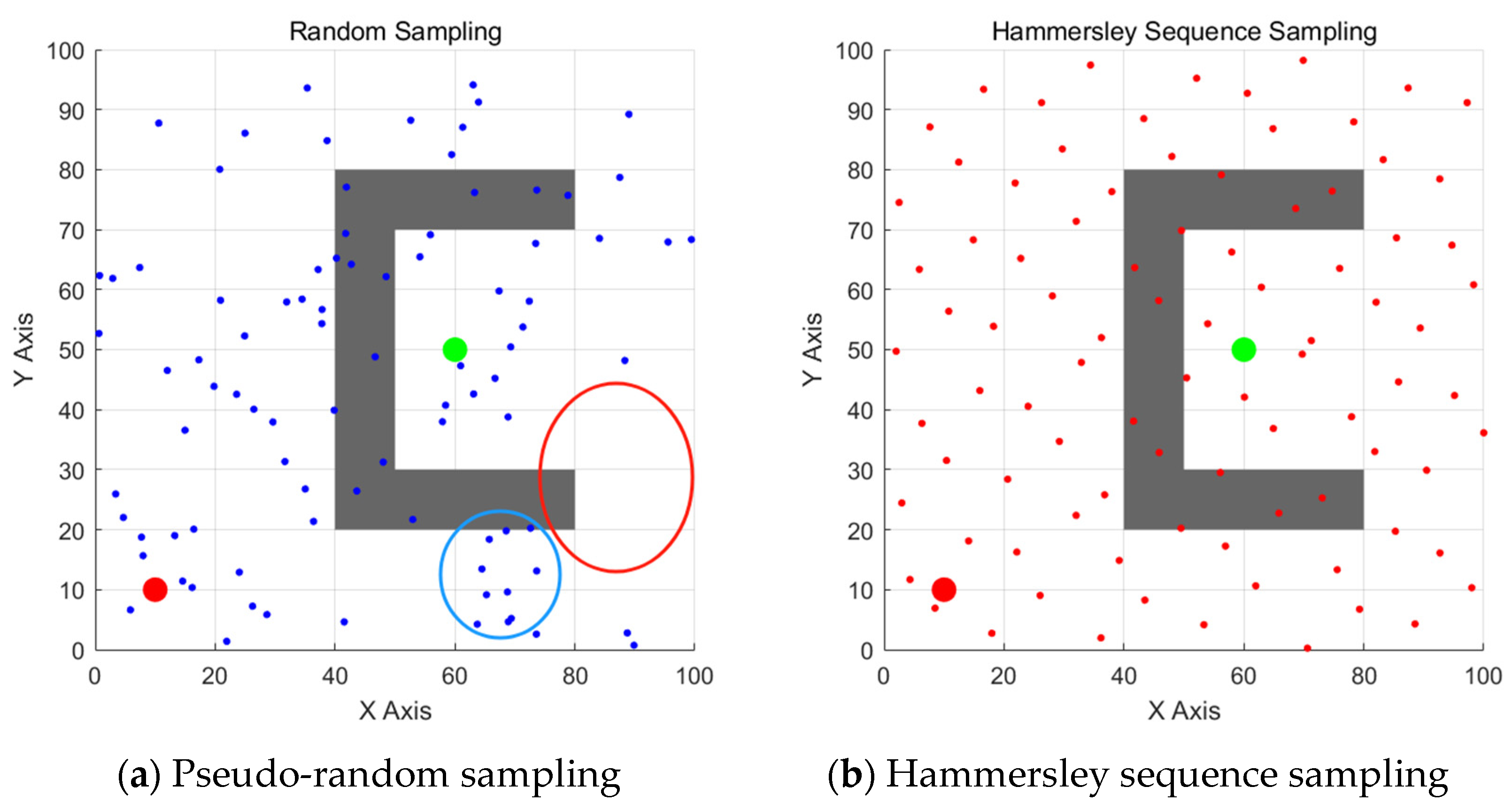
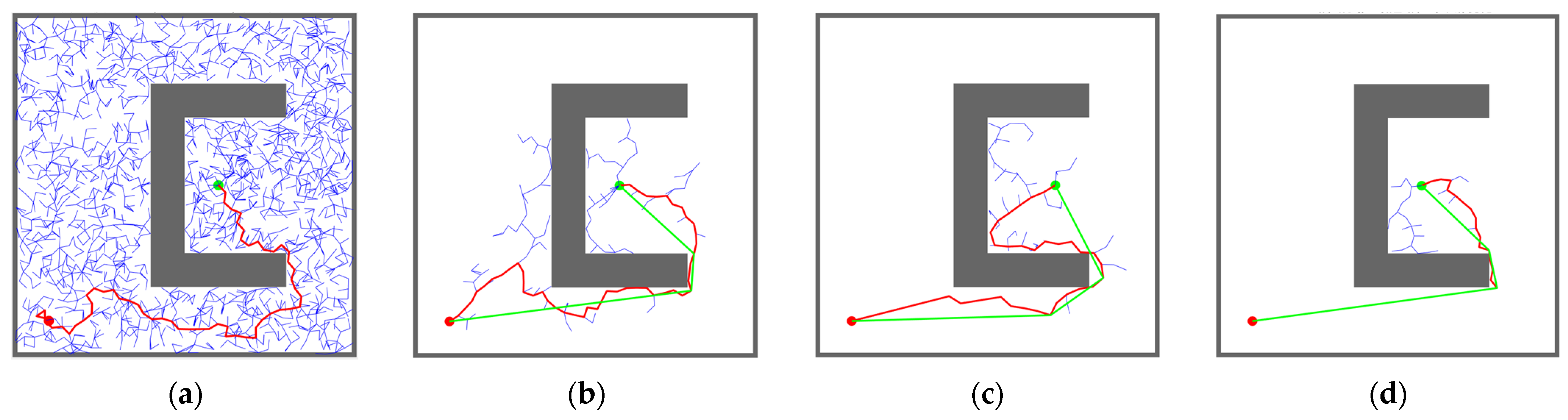
- Insufficient sampling in key regions: As shown in the red area in Figure 1a, due to the uneven probability density distribution of pseudo-random sampling, the algorithm struggles to consistently generate valid candidate points in key areas such as narrow passages. This prevents the heuristic function from filtering out suitable expansion nodes, significantly reducing the algorithm’s ability to break through semi-closed regions.
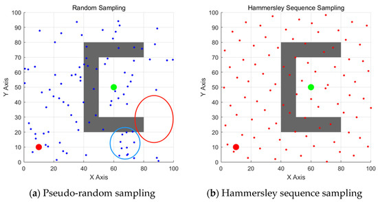 Figure 1. Comparison between pseudo-random sampling and Hammersley sequence sampling: (a) Pseudo-random sampling showing insufficient sampling in key regions (red area) and excessive sampling in redundant regions (blue area); (b) Hammersley sequence sampling demonstrating superior uniform distribution characteristics across the entire space.
 - Excessive sampling in redundant regions: As shown in the blue area in Figure 1a, sampling points exhibit non-uniform clustering phenomena. This excessive sampling in redundant regions not only wastes computational resources but also affects path planning efficiency due to the reduced spatial diversity of candidate points, forming a vicious cycle of increased computational overhead and decreased solution quality.
In contrast, as shown in Figure 1b, the point set generated by Hammersley sequence sampling exhibits superior uniform distribution characteristics. The MIHE-RRT algorithm breaks through the pseudo-random sampling limitations of traditional RRT by introducing the Hammersley sequence to achieve uniform spatial coverage. Unlike methods such as Neural RRT* which require pre-training processes, it ensures low computational overhead while maintaining high-quality sampling effects.
Research [26] indicates that Hammersley sequence sampling is an effective low-variance sequence sampling method that demonstrates superior point distribution uniformity in multidimensional spaces, effectively avoiding the point clustering and gap issues common in traditional Monte Carlo sampling. This uniform distribution characteristic not only ensures effective sampling in key regions but also prevents sampling point clustering, thereby enhancing the algorithm’s ability to break through complex regions while reducing computational overhead and improving path planning efficiency. This structured sampling method forms a complementary optimization with the heuristic search: while ensuring directional path exploration, it effectively eliminates the blind spots of random sampling through comprehensive spatial coverage characteristics, thereby achieving synergistic improvement in algorithm convergence speed and solution quality.
The generation method of Hammersley sequence sampling points is as follows:
- The first dimension adopts uniform distribution, and the equidistant selection is , where is the index of the sample, and the range is 1 to . is the number of samples.
- The second dimension employs the Van der Corput sequence with base to generate a low-variance sequence. The Van der Corput sequence transforms natural numbers into decimals within the interval [0, 1] through radix conversion and digit reversal, producing a uniformly distributed low-discrepancy sequence. The formula is as follows:
Here, represents the input natural number, is the base, and is the -th digit that will be represented as the base . Each point of the Hammersley sequence can be expressed as follows:
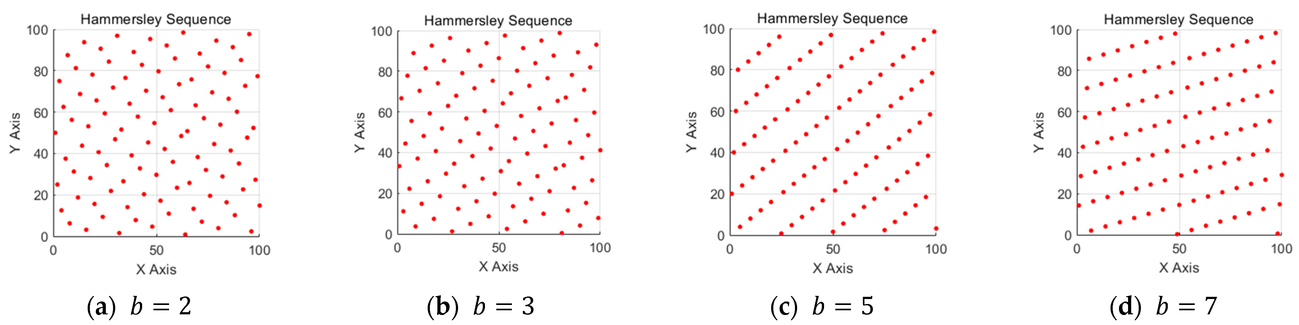
It is worth noting that the base is one of the key parameters for generating Hammersley sequence sampling points, which directly affects the distribution characteristics of the sequence in specific dimensions. Each dimension corresponds to a cardinal number, usually a prime number (such as 2, 3, 5, etc.). The choice of base has an important influence on the uniformity of point distribution and the coverage of multidimensional space. In the two-dimensional space of a 100 m × 100 m map, 100 points are generated by using prime numbers 2, 3, 5, and 7, respectively, and the distribution of observation points is observed.
It can be seen from Figure 2 that as b increases, the correlation between sampling points increases accordingly, while the distance between adjacent nodes decreases. At the same time, the sampling points will show a regular aggregation and some blank areas. Insufficient uniform sampling points will limit the global exploration ability of the tree, which may make the algorithm fall into the local minimum, unable to jump out of the constraints of complex obstacles and reduce the path quality and computational efficiency. Therefore, the Hammersley sequence with is selected for sampling.
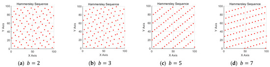
Figure 2.
Comparison of Hammersley sequence sampling with different base : (a) = 2 showing optimal uniform distribution with balanced spacing between points; (b) = 3 displaying slight clustering patterns beginning to emerge; (c) = 5 demonstrating increased correlation between sampling points with visible patterns; (d) = 7 showing further increased regularity and decreased uniformity with noticeable blank areas.
2.2. Multi-Indicator Heuristic Evaluation Mechanism
The core innovation of MIHE-RRT lies in proposing a multi-indicator heuristic evaluation mechanism, which fundamentally differs from the heuristic strategies used in existing RRT variants:
- Multi-dimensional collaborative evaluation: Existing algorithms such as Informed-RRT primarily rely on single-dimensional heuristic elliptical region sampling, while MIHE-RRT simultaneously considers three dimensions—spatial diversity, target distance, and directional angle—forming a more comprehensive evaluation system.
- Dynamic balancing mechanism: Through weight parameters (,), it achieves a dynamic balance between exploration and exploitation, solving the problem of excessive exploration in complex environments that occurs in other algorithms such as RRT.
- Integration of local and global information: The diversity value focuses on local spatial structure, the distance value guides the global target direction, and the angle value optimizes local expansion efficiency, achieving an organic integration of local and global information.
Based on the design concept of the above multi-indicator heuristic evaluation mechanism, the specific algorithm steps of MIHE-RRT are as follows:
- In the sampling phase, the point set of the Hammersley sequence sampling is generated in advance.
- For each point in the point set, calculate its Euclidean distance from all nodes in the current tree to find the nearest point .
- Move a step from to to obtain a new point .
- Check whether the path from to the nearest tree node is collision-free.
- Points where collisions occur will be deleted, while non-colliding points are retained. If all points in the set collide, the process advances to the next iteration.
- After completing collision detection, the remaining points in the set will become candidate points, with a quantity of k. The multi-indicator heuristic evaluation mechanism then calculates a value for each candidate point and selects the one with the highest value as the sampling point for the current iteration.
The value function combines the distance value , the angle value , and the diversity value . The formula is as follows:
The is the comprehensive value of the candidate point in the point set. , and are the weights for distance value, transition value, and diversity value, respectively.
2.2.1. Diversity Value
is the result of the normalization of the diversity value. The formula for is:
where is the candidate point and is the minimum distance from each candidate point to the tree. and are the maximum and minimum values of the minimum distances from all candidate points to the tree.
To optimize computational efficiency, only distances between candidate points and nodes in the local region are calculated. If there are no nodes in the local region, the distance to the nearest node is used as a reference. When is small (indicating proximity to the tree), approaches 0, reducing the probability of the candidate point being selected. When is large (indicating distance from the tree), approaches 1, increasing the probability of the candidate point being selected.
As shown in Figure 3, when only the diversity value is taken into account, the candidate point farthest from within the search radius will be selected as the final sampling point, which is .
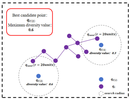
Figure 3.
Principle of diversity value: illustration showing how the candidate point farthest from the nearest tree node () within the search radius is selected as the sampling point () when considering only the diversity value indicator.
From a local efficiency perspective, distance-based point selection prevents node clustering and improves spatial coverage efficiency. From a global perspective, this approach enhances the algorithm’s exploration capability, facilitating the discovery of feasible paths while avoiding redundant distance calculations during tree expansion, thus improving overall algorithmic efficiency.
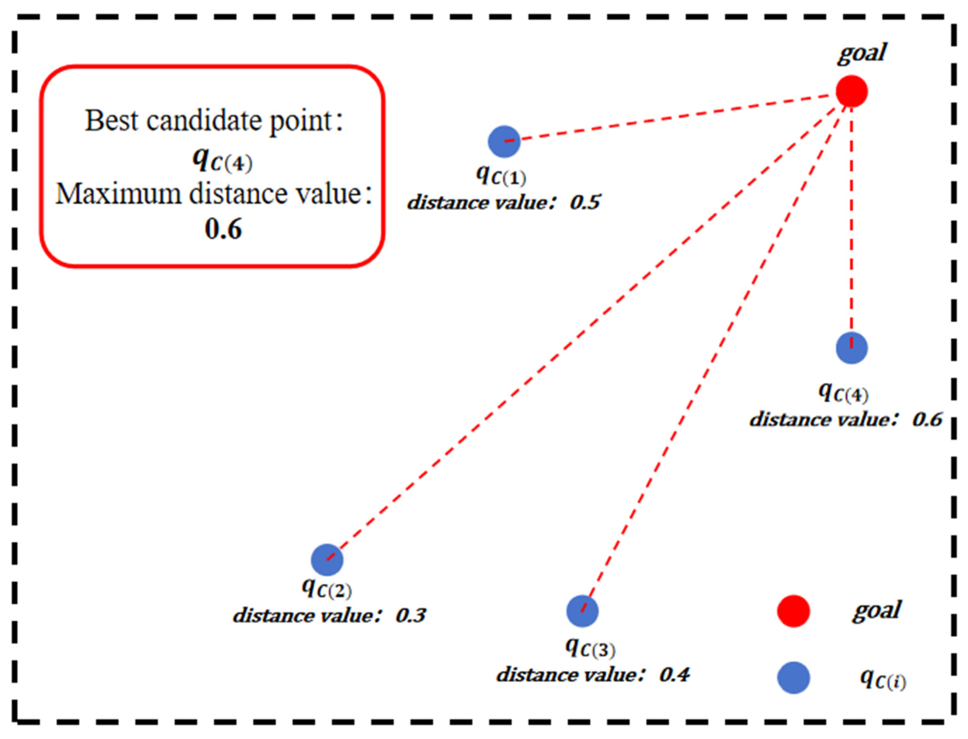
2.2.2. Distance Value
is the result of the normalization of the distance value. The formula for is
where is the target point. is the Euclidean distance between the candidate point and the target point.
represents the maximum distance in the environment. For a 100 m × 100 m map, the maximum distance corresponds to the diagonal length, m.
As shown in Figure 4, when only the distance value is considered, the candidate point with the smallest Euclidean distance from will be selected, which is , the final sampling point. The distance value ensures that the sampling point moves in the direction of the target.

Figure 4.
Principle of distance value: illustration demonstrating how the candidate point () with the smallest Euclidean distance to the target point () is selected as the final sampling point when considering only the distance value indicator, ensuring that sampling points move in the direction of the target.
2.2.3. Angle Value
is the result of the normalization of the angle value. The formula for is
where , represents the vector from the nearest node pointing to the target point , and represents the vector from the nearest node pointing to the candidate point .
As shown in Figure 5, when considering only the angle value, the candidate point with the minimum angle between vectors and is selected as the final sampling point. This angular metric evaluates the alignment between the extension direction and the target direction, which, combined with the distance value, optimizes path efficiency toward the target.
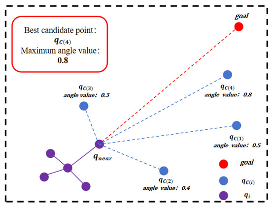
Figure 5.
Principle of angle value: illustration showing how the candidate point () with the minimum angle between vector A (from the nearest node to the target point ) and vector B (from the nearest node to the candidate point ) is selected as the final sampling point when considering only the angle value indicator, optimizing path efficiency toward the target.
2.2.4. Selection of Weights for Distance Value, Angle Value, and Diversity Value
From Equation (3), it can be known that represents the intensity of moving toward the target. The larger is, the stronger the intensity of moving toward the target, and the more direct it is to reach the target point. represents the alignment between the extension direction and the goal direction. As increases, it will purposefully guide the tree to grow toward the target. represents the control degree of spatial exploration. The larger is, the more spatial areas the path exploration covers, while also being able to avoid excessive exploration of failure areas.
In order to obtain the weights for the distance value, angle value, and diversity value that work most effectively in complex environments, the grid method is used for optimal weight selection.
First, we set the number of points in the point set to 50. For the grid search scheme, we set the ranges of , , and to [0.1, 0.8] with a step size of 0.1, and all combinations must satisfy + = 1, which generates 36 valid combinations. Each combination is tested 50 times on the map shown in Figure 6, which has a size of 200 m × 200 m. The average values of path length, time, and number of nodes are calculated for each combination. Finally, the top 5 combinations with the shortest time are selected for comprehensive comparison to determine the optimal weight combination.
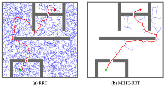
Figure 6.
The planning effect of the RRT algorithm and the path planning effect of the MIHE-RRT algorithm: (a) RRT algorithm showing extensive exploration with numerous nodes (blue dots) and a longer path (red line) from start point (green dot) to target point (red dot); (b) MIHE-RRT algorithm demonstrating more efficient planning with fewer nodes and a shorter path, while successfully navigating through the same environment.
The 5 combinations with the shortest time are shown in Table 2. It can be seen that when = 0.6, = 0.1, and = 0.3, the planning process requires the shortest time, the number of nodes is the lowest, and though the path length ranks third, it is not significantly different from the shortest path of 162.33 m. Comprehensively, = 0.6, = 0.1, and = 0.3 is selected as the weight for distance value, angle value, and diversity value in the subsequent testing process of the MIHE-RRT algorithm.
Table 2.
The 5 shortest time results.
2.2.5. The Number of Points in the Point Set ()
The number of points in the point set () generated by Hammersley sequence sampling significantly impacts the algorithm’s performance in terms of time, path length, and number of nodes. A small reduces computational complexity but may fail to identify high-quality candidate points. Conversely, a large increases the likelihood of finding high-quality candidates but substantially increases computational overhead and planning time. To determine the optimal , 50 experiments are conducted using MIHE-RRT in the environment shown in Figure 6, evaluating the trade-off between time, path length, and number of nodes.
As shown in Table 3, optimal planning performance is achieved when the Hammersley sequence generates 25 points, resulting in a path length of 173.29 m, planning time of 0.036 s, and average node count of 211.13.
Table 3.
Planning results under different numbers of generated points in Hammersley sequence sampling.
Figure 6 presents a comparative analysis between the RRT and MIHE-RRT algorithms. While both algorithms successfully reach the endpoint, Figure 6a demonstrates that the RRT algorithm requires significantly more nodes and produces longer paths than MIHE-RRT. Figure 6b illustrates that MIHE-RRT, through its value-based sampling point selection, achieves superior performance with fewer nodes and shorter paths, particularly effective in navigating complex and narrow environments.
2.3. Tree Pruning
The initial path generated by the RRT algorithm is formed by connecting randomly sampled points with straight lines, which typically contain redundant nodes and unnecessary turns. In order to improve path efficiency, it is necessary to optimize and simplify it.
The optimization process adopts a segment-by-segment detection method: starting from the starting point of the path, the algorithm attempts to directly connect to further path points. For each attempted straight-line connection, the system will perform collision detection. If the straight path does not collide with any obstacles, all intermediate nodes between these two points can be deleted; if a collision occurs, keep the last safely reachable node as the new starting point and continue optimizing the subsequent path segments.
The RRT algorithm initially generates a path by connecting randomly sampled points with straight-line segments, resulting in redundant nodes and suboptimal turns. Path optimization is necessary to improve efficiency.
The optimization employs an iterative segment detection approach:
- Beginning at the path’s start point, the algorithm attempts to establish direct connections to subsequent path points.
- Each potential straight-line connection undergoes collision detection.
- If no obstacle collisions are detected, all intermediate nodes between the connected points are eliminated.
- If a collision is detected, the last valid (collision-free) node becomes the new starting point for optimizing the remaining segments.
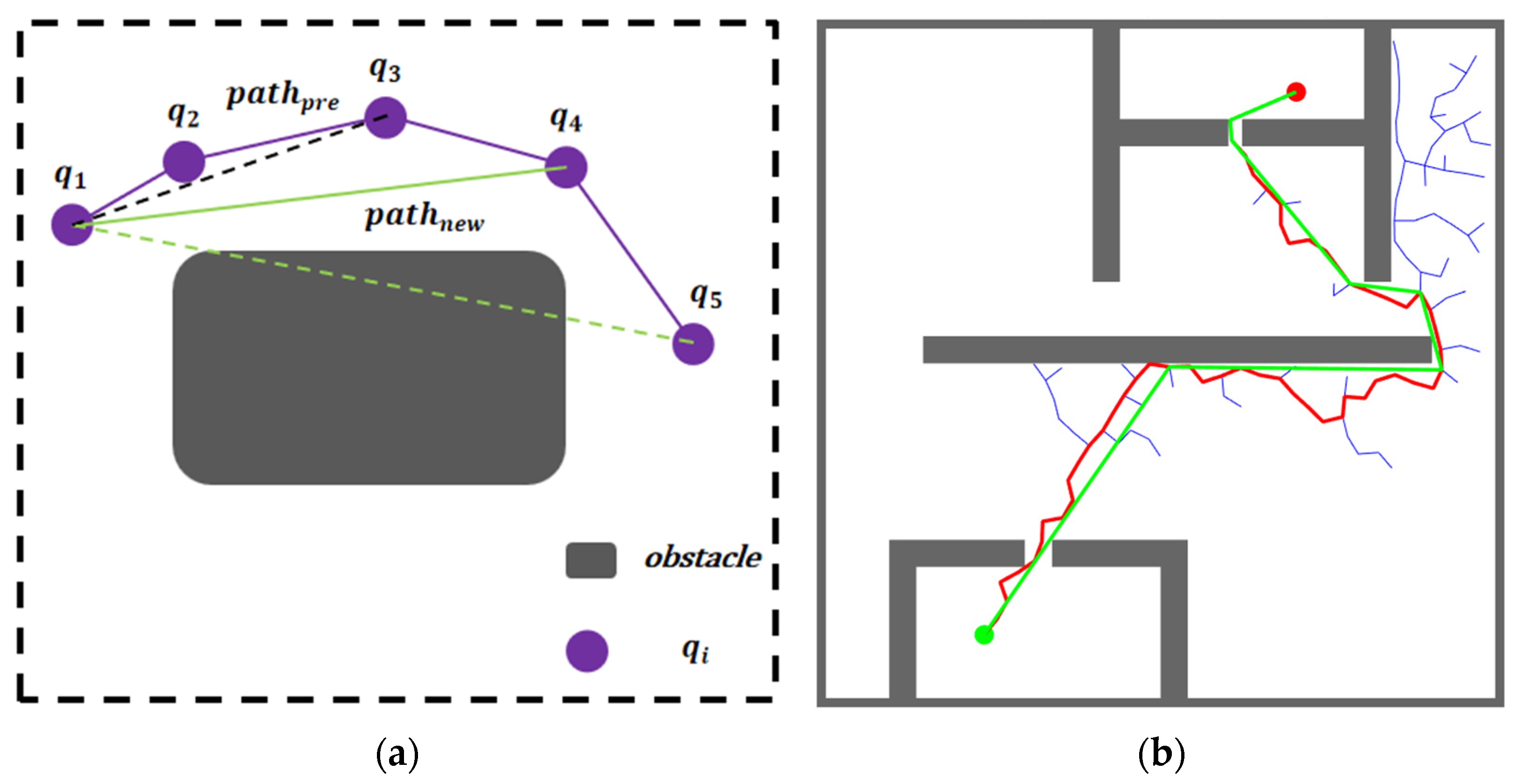
As shown in Figure 7a, where represents the node position, represents the initial path generated by the RRT algorithm; represents the optimized path. The dark gray rounded rectangle represents obstacles.
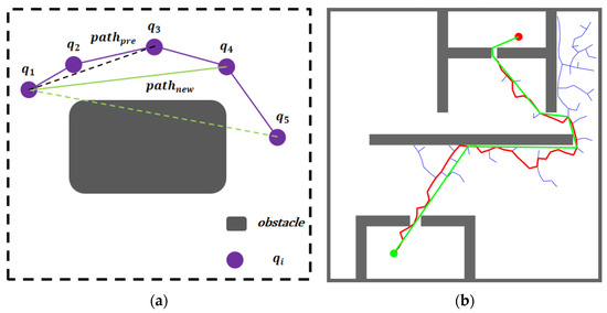
Figure 7.
Path-smoothing principle diagram and actual effect diagram: (a) Illustration of the path-smoothing principle showing the optimization process from initial path to smoothed path; (b) Comparison between the initial path and the optimized path after applying the tree pruning algorithm.
Starting from , the optimization process attempts to establish direct connections to subsequent nodes. In Figure 7a, while the attempted path from to collides with obstacles, the connection between and remains collision-free and is selected as the optimized segment. The optimization then continues with as the new starting point.
Figure 7b illustrates the optimized path (shown in green), which demonstrates significant improvements over the initial path. Through iterative segment detection and collision checking, the algorithm eliminates redundant nodes and unnecessary turns while maintaining path safety. This optimization process substantially reduces path length while preserving feasibility.
2.4. Computational Complexity
2.4.1. Space Complexity
The space complexity of the MIHE-RRT algorithm can be determined by analyzing the key data structures and storage requirements during algorithm execution:
- The main space requirement comes from storing the random tree structure. Each node needs to store coordinate position, parent node reference, comprehensive value, and node connections. If is the total number of nodes in the final tree, this part requires space.
- The algorithm generates 25 candidate points in each iteration using Hammersley sequence sampling. These 25 points are temporarily stored for evaluation. This is a fixed space requirement of , as the sample size remains fixed at 25 regardless of the input scale.
- For heuristic evaluation, the algorithm needs to store diversity value, distance value, and angle value for each candidate point, as well as weight parameters (,) and comprehensive evaluation scores. Since these values are calculated for a fixed number of candidate points (25), this also requires space.
- Once the algorithm finds a path, it needs to store the path. Storing the final path as a sequence of nodes and the optimized pruned path requires, in the worst case, space as the path might include all nodes in the tree.
- For collision detection, the algorithm needs to maintain a representation of obstacles in the environment and temporary variables for collision checking. The space complexity of the environment representation depends on the specific implementation but is typically , where is the number of obstacles.
Overall, the total space complexity of the MIHE-RRT algorithm is , primarily determined by the random tree structure and environment representation.
2.4.2. Time Complexity
For each iteration, the following apply:
- When generating the point set during each of the 25 iterations, each step includes sampling point generation , finding the nearest neighbor , and collision detection . The overall time complexity is , which simplifies to , where represents the current number of nodes in the tree.
- In the best candidate selection phase of the algorithm, we need to select the optimal point from candidates that have passed collision detection. This process requires performing multiple operations for each candidate point: calculating its distance to the target , finding the nearest node to it in the tree , determining the relevant nodes in the local small-scale search area , and calculating various value metrics . Combining these operations, the theoretical time complexity for selecting the best candidate point is .
- In the step of generating a new node, extending the nearest node toward the sampling point based on the specified step length is a basic mathematical operation with a time complexity of .
- Finally, the algorithm adds the new node to the tree structure, which only involves the simple addition of array elements and calculation of cost values, a constant time operation with complexity .
- Therefore, the total complexity for a single iteration is . Simplified to , and since 25 and are constants, the final complexity is .
3. Experimental Simulation Results and Analysis
Section 3.1 introduces the prerequisites for simulation testing. Section 3.2 introduces the performance comparison of the MIHE-RRT algorithm on Map 1 (semi-closed), Map 2 (maze), Map 3 (chaotic), and Map 4 (crowded). The comparative tests include the RRT algorithm, IBi-RRT, and HB-RRT algorithm.
3.1. Preparation for Simulation Testing
The simulation study utilized MATLAB 2021b (MathWorks, Natick, MA, USA) running on a computer equipped with an Intel Core i7-10875H processor (2.3 GHz CPU frequency, Intel Corporation, Santa Clara, CA, USA) and 16 GB RAM.
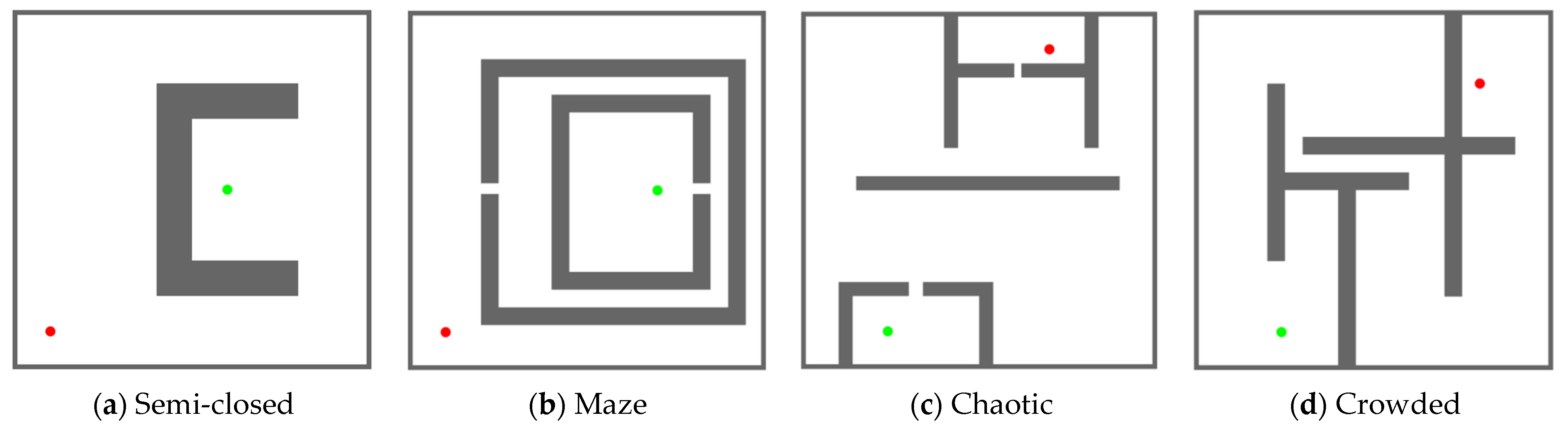
The MIHE-RRT algorithm underwent 50 test iterations on four distinct maps, with standard RRT algorithm, IBi-RRT, and HB-RRT algorithm tested for comparison. Results represent averages across all 50 tests. As illustrated in Figure 8, each map (all sized 200 m × 200 m) was designed to evaluate specific capabilities.
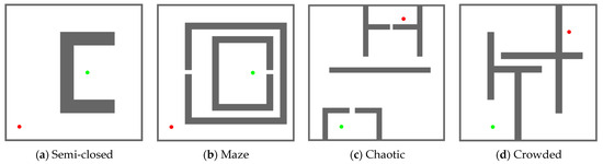
Figure 8.
Four types of maps for simulation testing: (a) Semi-closed environment with a narrow pathway surrounded by obstacles, designed to test the algorithm’s ability to escape dead zones; (b) Maze environment with continuous narrow passages and multiple dead ends, testing navigation capabilities in constrained spaces; (c) Chaotic environment with irregularly distributed obstacles, examining adaptability to complex spatial structures; (d) Crowded environment with multiple obstacles creating narrow passages between them, challenging the algorithm’s efficiency in multi-objective scenarios. In all maps, the green dot represents the starting point and the red dot represents the target point, with obstacles shown in brown.
Map 1 evaluated the algorithm’s efficiency in escaping dead zones and path planning in open areas, testing its adaptability to varying environmental characteristics. Map 2 assessed navigation through narrow channels, testing the algorithm’s handling of continuous turns and dead ends. Map 3 evaluated performance amid irregularly distributed obstacles, examining adaptability to complex spatial structures. Map 4 challenged the algorithm’s planning capabilities in multi-objective environments, particularly its efficiency in navigating narrow passages.
In the visualizations, starting points were indicated by green dots, target points by red dots, and optimized paths by green lines, with obstacles shown in brown. All algorithms were configured with 15,000 iterations and a 4 m step size. For IBi-RRT, the attractive force coefficient is set to 1.5, and the probability threshold is set to 0.2. For HB-RRT, the candidate pool size is 30, and .
The evaluation framework centered on three critical performance metrics:
Path length (m) serves as an indicator of the algorithm’s pathfinding quality and optimization capabilities. Computation time (s) demonstrates real-time performance, directly impacting robot response speed—a crucial factor for real-time control systems. The number of nodes reflects computational complexity and resource utilization, where fewer nodes indicate more efficient searching and reduced system load, ultimately affecting the robot’s operational efficiency.
These three interconnected metrics collectively determine the algorithm’s practical utility. Their relationships and combined effects provide a comprehensive measure of the algorithm’s real-world applicability in robotic systems.
3.2. Algorithm Simulation Testing
The performance of the MIHE-RRT algorithm was evaluated in four different map environments (semi-closed, maze, chaotic, and crowded), and compared with the RRT, IBi-RRT, and HB-RRT algorithms. The experiments comprehensively analyzed the efficiency and effectiveness of the algorithm through path length (m), time (s), and number of nodes.
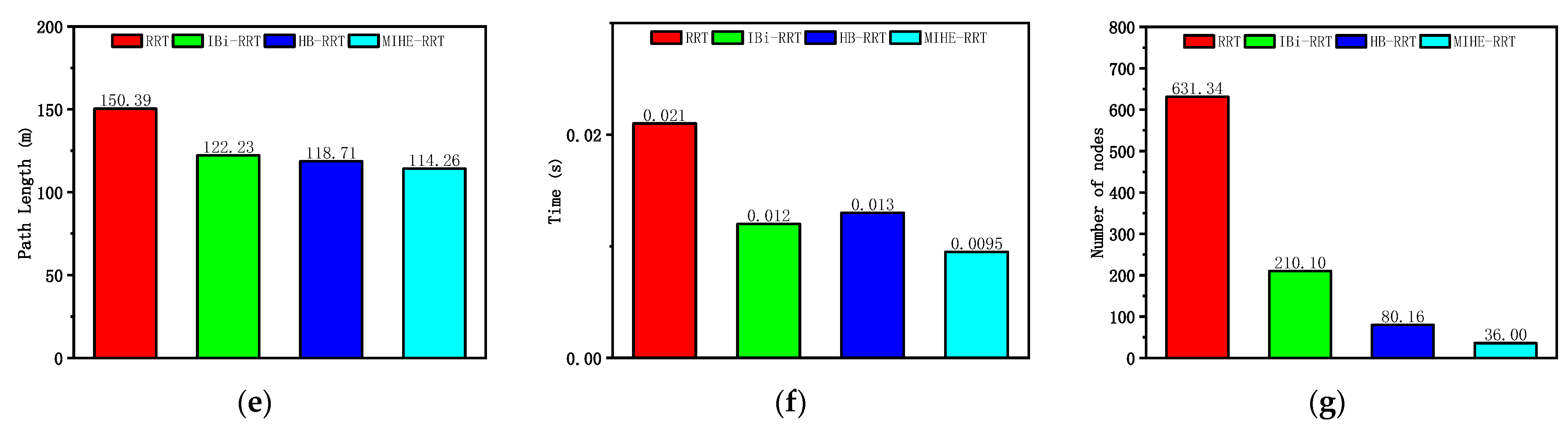
According to the analysis of the results in Figure 9 and Table 4, the MIHE-RRT algorithm exhibits comprehensive performance advantages in semi-closed environments. In terms of execution efficiency, MIHE-RRT achieves an average time of 0.0095 s, which is notably faster than its competitors—54.76% faster than the original RRT’s 0.021 s, 20.83% faster than IBi-RRT’s 0.012 s, and 26.92% faster than HB-RRT’s 0.013 s.
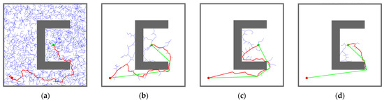

Figure 9.
Simulation results and statistical results (Map 1): (a) Path planning result of RRT algorithm; (b) Path planning result of IBi-RRT algorithm; (c) Path planning result of HB-RRT algorithm; (d) Path planning result of MIHE-RRT algorithm; (e) Comparison of path length; (f) Comparison of computation time; (g) Comparison of number of nodes.
Table 4.
Comparison of algorithm performance (Map 1).
Regarding path planning quality, MIHE-RRT generates an average path length of 114.26 m, outperforming other algorithms with paths that are 24.02% shorter than RRT’s 150.39 m, 6.52% shorter than IBi-RRT’s 122.23 m, and 3.74% shorter than HB-RRT’s 118.70 m. In terms of computational resource consumption, MIHE-RRT requires significantly fewer nodes, averaging 36 nodes compared to RRT’s 631.34 (94.30% reduction), IBi-RRT’s 210.1 (82.87% reduction), and HB-RRT’s 80.16 (55.09% reduction).
The stability metrics of MIHE-RRT also show marked improvement, with time fluctuations controlled between 0.0077 and 0.012 s, and path length variations limited between 110.61 m and 121.76 m, demonstrating MIHE-RRT’s superior consistency in performance.
According to the analysis of the results in Figure 10 and Table 5, the MIHE-RRT algorithm demonstrates comprehensive performance advantages in the maze environment. In terms of execution efficiency, MIHE-RRT achieves an average time of 0.074 s, which is notably faster than its competitors—70.40% faster than the original RRT’s 0.25 s, 53.75% faster than IBi-RRT’s 0.16 s, and 72.59% faster than HB-RRT’s 0.27 s.
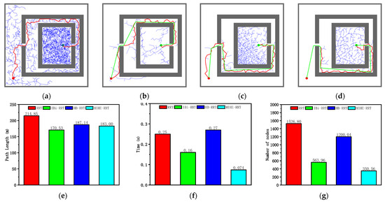
Figure 10.
Simulation results and statistical results (Map 2): (a) Path planning result of RRT algorithm; (b) Path planning result of IBi-RRT algorithm; (c) Path planning result of HB-RRT algorithm; (d) Path planning result of MIHE-RRT algorithm; (e) Comparison of path length; (f) Comparison of computation time; (g) Comparison of number of nodes.
Table 5.
Comparison of algorithm performance (Map 2).
Regarding path planning quality, MIHE-RRT generates an average path length of 183 m, outperforming most algorithms which have paths that are 14.82% shorter than RRT’s 214.85 m and 2.21% shorter than HB-RRT’s 187.14 m, though it is 7.31% longer than IBi-RRT’s 170.53 m. In terms of computational resource consumption, MIHE-RRT requires significantly fewer nodes, averaging 350.36 nodes compared to RRT’s 1526.8 (77.05% reduction), IBi-RRT’s 563.96 (37.87% reduction), and HB-RRT’s 1200.04 (70.81% reduction).
The stability metrics of MIHE-RRT also show marked improvement, with time fluctuations controlled between 0.036 and 0.23 s, and path length variations limited between 176.36 m and 188.06 m, demonstrating MIHE-RRT’s superior consistency in performance.
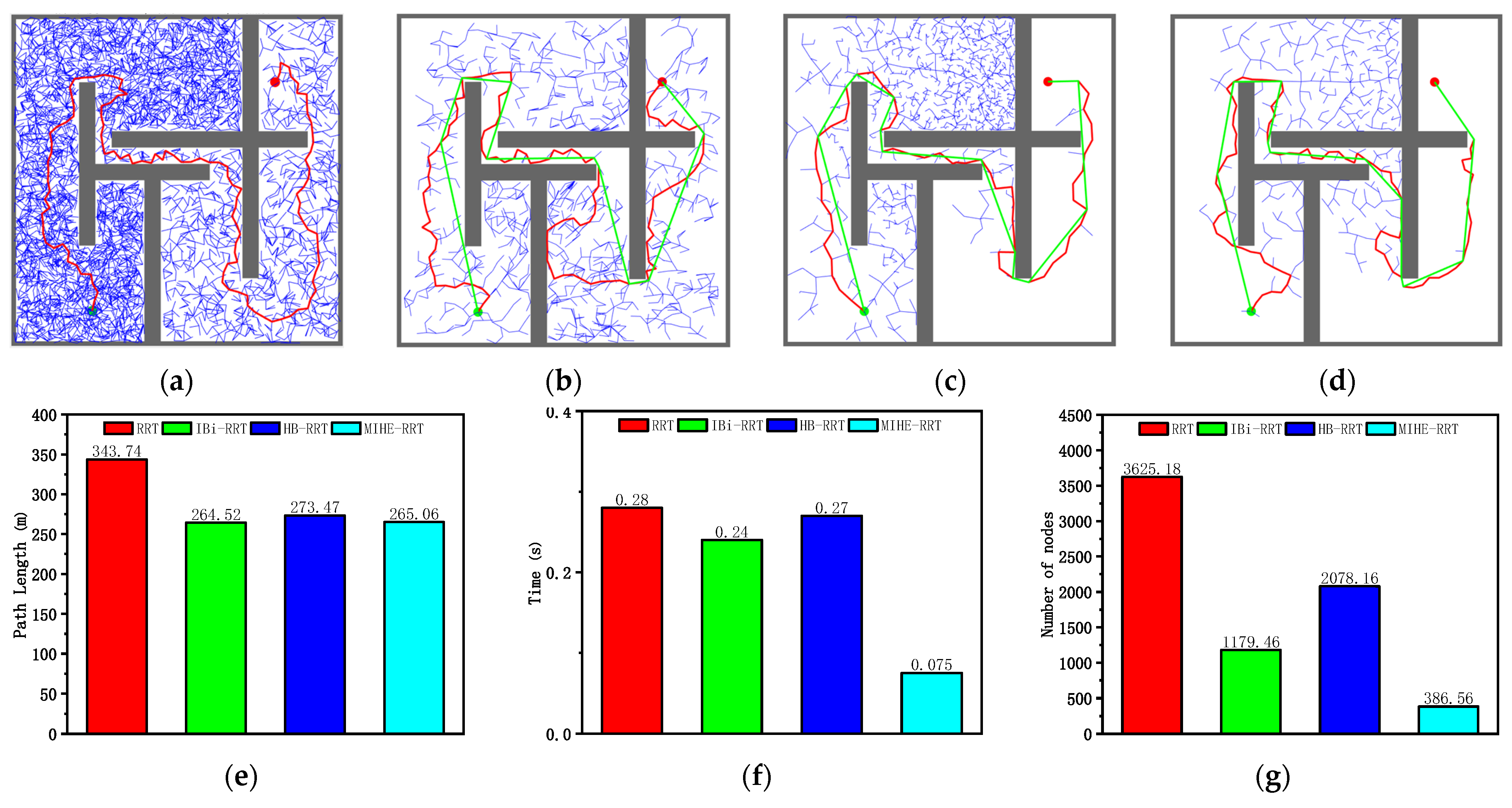
According to the analysis of the results in Figure 11 and Table 6, the MIHE-RRT algorithm demonstrates comprehensive performance advantages in the chaotic environment. In terms of execution efficiency, MIHE-RRT achieves an average time of 0.075 s, which is notably faster than its competitors—73.21% faster than the original RRT’s 0.28 s, 68.75% faster than IBi-RRT’s 0.24 s, and 72.22% faster than HB-RRT’s 0.27 s.

Figure 11.
Simulation results and statistical results (Map 3): (a) Path planning result of RRT algorithm; (b) Path planning result of IBi-RRT algorithm; (c) Path planning result of HB-RRT algorithm; (d) Path planning result of MIHE-RRT algorithm; (e) Comparison of path length; (f) Comparison of computation time; (g) Comparison of number of nodes.
Table 6.
Comparison of algorithm performance (Map 3).
Regarding path planning quality, MIHE-RRT generates an average path length of 265.06 m, outperforming most algorithms with paths that are 22.89% shorter than RRT’s 343.74 m and 3.08% shorter than HB-RRT’s 273.47 m, though it is marginally longer (0.20%) than IBi-RRT’s 264.52 m. In terms of computational resource consumption, MIHE-RRT requires significantly fewer nodes, averaging 386.56 nodes compared to RRT’s 3625.18 (89.34% reduction), IBi-RRT’s 1179.46 (67.23% reduction), and HB-RRT’s 2078.16 (81.40% reduction).
The stability metrics of MIHE-RRT also show marked improvement, with time fluctuations controlled between 0.057 and 0.12 s, and path length variations limited between 248.99 m and 292.69 m, demonstrating MIHE-RRT’s superior consistency in performance.
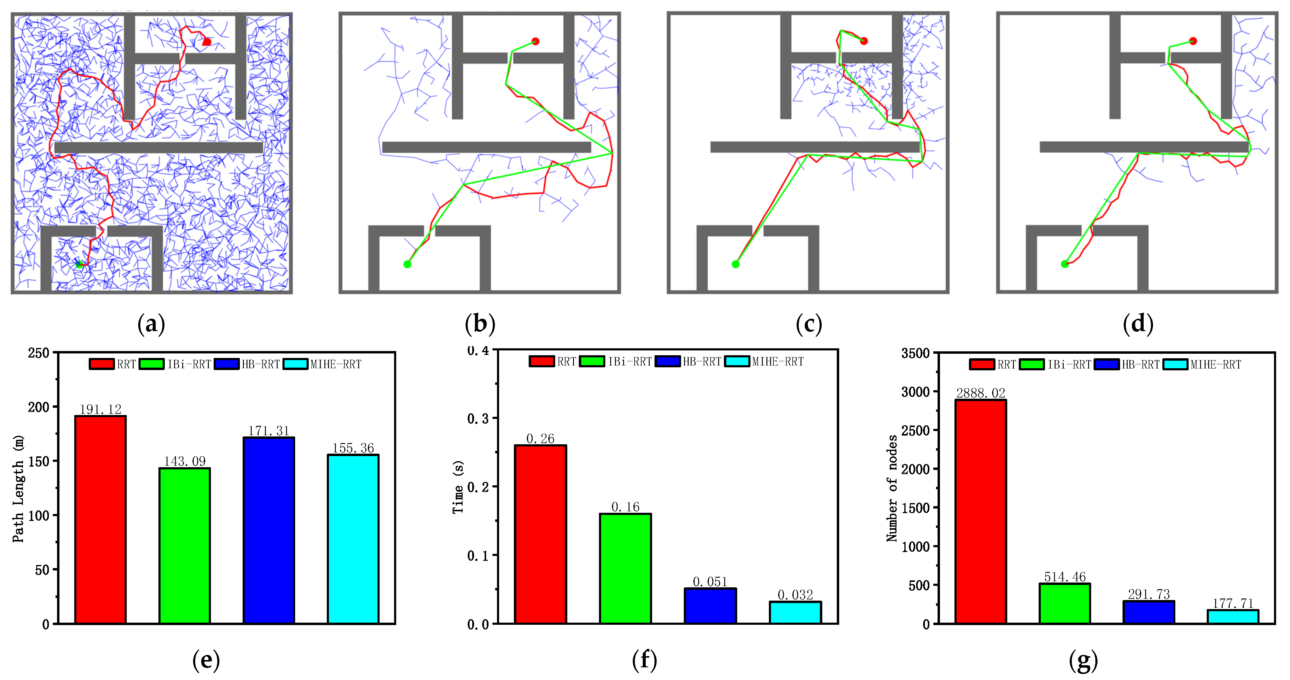
According to the analysis of the results in Figure 12 and Table 7, the MIHE-RRT algorithm maintains comprehensive performance advantages in the crowded environment. In terms of execution efficiency, MIHE-RRT achieves an average time of 0.032 s, which is substantially faster than its competitors—87.69% faster than RRT’s 0.26 s, 80% faster than IBi-RRT’s 0.16 s, and 37.25% faster than HB-RRT’s 0.051 s.
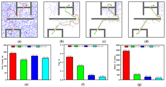
Figure 12.
Simulation results and statistical results (Map 4): (a) Path planning result of RRT algorithm; (b) Path planning result of IBi-RRT algorithm; (c) Path planning result of HB-RRT algorithm; (d) Path planning result of MIHE-RRT algorithm; (e) Comparison of path length; (f) Comparison of computation time; (g) Comparison of number of nodes.
Table 7.
Comparison of algorithm performance (Map 4).
Regarding path planning quality, MIHE-RRT generates an average path length of 155.36 m, which is 18.71% shorter than RRT’s 191.12 m and 9.31% shorter than HB-RRT’s 171.31 m, though slightly longer (8.57%) than IBi-RRT’s 143.09 m. In terms of computational resource consumption, MIHE-RRT requires significantly fewer nodes, averaging 177.71 nodes compared to RRT’s 2888.02 (93.84% reduction), IBi-RRT’s 514.46 (65.46% reduction), and HB-RRT’s 291.73 (39.09% reduction).
The stability metrics of MIHE-RRT continue to excel, with time fluctuations controlled within 0.016 to 0.13 s and path length variations limited between 147.63 m and 168.76 m, both significantly better than other algorithms. These comprehensive results demonstrate MIHE-RRT’s ability to maintain excellent performance and stability across diverse environments, underscoring its practical value in path planning applications.
4. Conclusions and Future Directions
The MIHE-RRT algorithm proposed in this study demonstrates significant innovation in two aspects:
- Sampling strategy innovation: Compared to pseudo-random sampling used by traditional RRT, RRT*, and IBi-RRT, Hammersley sequence sampling provides theoretically superior spatial coverage characteristics; compared to the Halton sequence used by HB-RRT, the Hammersley sequence exhibits more uniform distribution properties in low-dimensional spaces. This study designed an innovative algorithm based on Hammersley sequence sampling that can generate high-quality point sets with uniform distribution and low discrepancy, providing a solid foundation for subsequent multi-indicator heuristic evaluation. By optimizing sampling point distribution, the algorithm significantly reduces redundant sampling in open areas, allowing computational resources to be allocated more rationally, thereby improving overall efficiency. Compared to traditional sampling methods, the Hammersley sequence provides more consistent spatial coverage characteristics, making the exploration process more efficient.
- Evaluation mechanism innovation: Unlike existing algorithms that rely on single evaluation metrics (such as probability thresholds or path length), the MIHE-RRT in this study introduces a three-dimensional evaluation system to achieve a comprehensive assessment of candidate points. When encountering obstacles, this study implements diversity values in the algorithm to prevent efficiency loss by avoiding excessive exploration of specific areas, enabling it to effectively bypass obstacles and escape challenging situations. This study combines distance and angle values to more purposefully guide tree growth toward the target, optimizing sampling point distribution and reducing redundant sampling in open areas. Through multi-indicator heuristic evaluation, this study achieves efficient path planning in complex regions. After generating the path, this study uses MIHE-RRT’s tree pruning algorithm to delete unnecessary nodes, thereby optimizing the global path length.
The experiments compared MIHE-RRT with standard RRT, IBi-RRT, and HB-RRT algorithms in four environments (semi-enclosed, maze, chaotic, and crowded). Results show that MIHE-RRT demonstrates significant advantages in key performance metrics. In terms of execution efficiency, MIHE-RRT is 54–88% faster than other algorithms, with the most notable improvement in crowded environments. Regarding path quality, path lengths are reduced by 15–24% compared to RRT, and while slightly inferior to IBi-RRT in certain scenarios, it shows more stable overall performance. In terms of computational resources, the required number of nodes is significantly reduced by 77–94%, greatly improving computational efficiency. Additionally, MIHE-RRT shows minimal fluctuations in path length and execution time across all test scenarios, demonstrating excellent algorithm stability. It effectively addresses the sampling efficiency, balance, and computational resource problems mentioned in the introduction, providing a robust solution for robot path planning in complex environments.
The future research focus of the MIHE-RRT algorithm as a path planning method centers on four directions: First, we will enhance its adaptability to dynamic environments by adjusting sampling strategies and evaluation weights in real time, enabling the algorithm to better respond to environmental changes. Second, we will conduct algorithm comparison and integration research by comparing MIHE-RRT with the RRT algorithm mentioned in the research [27], the BIV* algorithm [28], the ARRT-Connect algorithm [29], and other types of path planning algorithms. Through this comparison, we will explore the potential of algorithm integration and develop hybrid algorithms with superior performance. Finally, we will extend the algorithm to three-dimensional applications and implement parallel computing optimization to improve its practicality and operational efficiency in large-scale scenarios.
It should be noted that the verification in this study was based solely on computer simulation without physical experiments, primarily limited by the following factors: lack of suitable robotic platforms and facilities for testing in complex environments, resources required for constructing physical test environments (such as maze and semi-closed environments) exceeding the current research budget, and sensor uncertainties and mechanical execution errors in real environments introducing additional variables. We recognize the importance of physical verification and plan to implement it in two phases in the future: first validating core algorithm functionalities in small-scale laboratory environments, then conducting larger-scale tests in actual scenarios with industry partners to address various challenges in the transition from simulation to actual deployment of the algorithm.
Author Contributions
Conceptualization, W.W., C.K. and Z.X.; data curation, C.K. and Q.H.; investigation, W.W., M.Y., Z.R. and Q.H.; methodology, W.W., C.K. and Z.X.; visualization, W.W., M.Y., Z.R. and Q.H.; writing—original draft, C.K.; writing—review and editing, W.W., C.K. and Z.X. All authors have read and agreed to the published version of the manuscript.
Funding
This research was funded by the Guangdong Provincial Department of Education Project under grant 2021ZDZX1020 and the Guangzhou Municipal Education Bureau’s Higher Education Research Project under grant 202235237.
Data Availability Statement
The data are included in the article.
Acknowledgments
The authors extend their appreciation to the Guangdong Provincial Government for funding this work via the Guangdong Provincial Department of Education Project under grant 2021ZDZX1020 and the Guangzhou Municipal Education Bureau for supporting this study through the Guangzhou Municipal Education Bureau’s Higher Education Research Project under grant 202235237.
Conflicts of Interest
The authors declare that they have no conflicts of interest.
References
- Dai, Y.; Li, S.; Rui, X.; Xiang, C.; Nie, X. Review of key technologies of climbing robots. Front. Mech. Eng. 2023, 18, 48. [Google Scholar] [CrossRef]
- Xu, Y.; Guan, G.; Song, Q.; Jiang, C.; Wang, L. Heuristic and random search algorithm in optimization of route planning for Robot’s geomagnetic navigation. Comput. Commun. 2020, 154, 12–17. [Google Scholar] [CrossRef]
- Zhang, Z.; Jiang, J.; Wu, J.; Zhu, X. Efficient and optimal penetration path planning for stealth unmanned aerial vehicle using minimal radar cross-section tactics and modified A-Star algorithm. ISA Trans. 2023, 134, 42–57. [Google Scholar] [CrossRef]
- Kavraki, L.E.; Kolountzakis, M.N.; Latombe, J.-C. Analysis of probabilistic roadmaps for path planning. IEEE Trans. Robot. Autom. 1998, 14, 166–171. [Google Scholar] [CrossRef]
- Li, Y.; Wei, W.; Gao, Y.; Wang, D.; Fan, Z. PQ-RRT*: An improved path planning algorithm for mobile robots. Expert Syst. Appl. 2020, 152, 113425. [Google Scholar] [CrossRef]
- Khatib, O. Real-time obstacle avoidance for manipulators and mobile robots. Int. J. Robot. Res. 1986, 5, 90–98. [Google Scholar] [CrossRef]
- Montiel, O.; Orozco-Rosas, U.; Sepúlveda, R. Path planning for mobile robots using bacterial potential field for avoiding static and dynamic obstacles. Expert Syst. Appl. 2015, 42, 5177–5191. [Google Scholar] [CrossRef]
- Tu, J.; Yang, S.X. Genetic algorithm based path planning for a mobile robot. In Proceedings of the 2003 IEEE International Conference on Robotics and Automation (Cat. No. 03CH37422), Taipei, Taiwan, 14–19 September 2003; pp. 1221–1226. [Google Scholar]
- Zhang, X.; Xia, S.; Zhang, T.; Li, X. Hybrid FWPS cooperation algorithm based unmanned aerial vehicle constrained path planning. Aerosp. Sci. Technol. 2021, 118, 107004. [Google Scholar] [CrossRef]
- LaValle, S. Rapidly-Exploring Random Trees: A New Tool for Path Planning; Research Report 9811; Iowa State University: Ames, IA, USA, 1998. [Google Scholar]
- Karaman, S.; Frazzoli, E. Sampling-based algorithms for optimal motion planning. Int. J. Robot. Res. 2011, 30, 846–894. [Google Scholar] [CrossRef]
- Kuffner, J.J.; LaValle, S.M. RRT-connect: An efficient approach to single-query path planning. In Proceedings of the 2000 ICRA. Millennium Conference. IEEE International Conference on Robotics and Automation. Symposia Proceedings (Cat. No. 00CH37065), San Francisco, CA, USA, 24–28 April 2000; pp. 995–1001. [Google Scholar]
- Gammell, J.D.; Srinivasa, S.S.; Barfoot, T.D. Informed RRT*: Optimal sampling-based path planning focused via direct sampling of an admissible ellipsoidal heuristic. In Proceedings of the 2014 IEEE/RSJ International Conference on Intelligent Robots and Systems, Chicago, IL, USA, 14–18 September 2014; pp. 2997–3004. [Google Scholar]
- Ye, L.; Li, J.; Li, P. Improving path planning for mobile robots in complex orchard environments: The continuous bidirectional Quick-RRT* algorithm. Front. Plant Sci. 2024, 15, 1337638. [Google Scholar] [CrossRef]
- Wang, B.; Ju, D.; Xu, F.; Feng, C.; Xun, G. CAF-RRT*: A 2D path planning algorithm based on circular arc fillet method. IEEE Access 2022, 10, 127168–127181. [Google Scholar]
- Zhong, H.; Cong, M.; Wang, M.; Du, Y.; Liu, D. HB-RRT: A path planning algorithm for mobile robots using Halton sequence-based rapidly-exploring random tree. Eng. Appl. Artif. Intell. 2024, 133, 108362. [Google Scholar] [CrossRef]
- Mashayekhi, R.; Idris, M.Y.I.; Anisi, M.H.; Ahmedy, I. Hybrid RRT: A semi-dual-tree RRT-based motion planner. IEEE Access 2020, 8, 18658–18668. [Google Scholar] [CrossRef]
- Liang, Y.-m.; Zhao, H.-y. CCPF-RRT*: An improved path planning algorithm with consideration of congestion. Expert Syst. Appl. 2023, 228, 120403. [Google Scholar]
- Wang, J.; Li, J.; Song, Y.; Tuo, Y.; Liu, C. FC-RRT*: A modified RRT* with rapid convergence in complex environments. J. Comput. Sci. 2024, 77, 102239. [Google Scholar]
- Zhang, M.; Chen, Y.; Luo, S.; Li, Q.; Zhao, H.; Zu, L. Path Planning of The Robotic Manipulator Based on An Improved Bi-RRT. IEEE Sens. J. 2024, 24, 31245–31261. [Google Scholar]
- Wang, J.; Chi, W.; Li, C.; Wang, C.; Meng, M.Q.-H. Neural RRT*: Learning-based optimal path planning. IEEE Trans. Autom. Sci. Eng. 2020, 17, 1748–1758. [Google Scholar] [CrossRef]
- Yuan, C.; Zhang, W.; Liu, G.; Pan, X.; Liu, X. A heuristic rapidly-exploring random trees method for manipulator motion planning. IEEE Access 2019, 8, 900–910. [Google Scholar]
- Huang, T.; Fan, K.; Sun, W. Density gradient-RRT: An improved rapidly exploring random tree algorithm for UAV path planning. Expert Syst. Appl. 2024, 252, 124121. [Google Scholar] [CrossRef]
- Fan, J.; Chen, X.; Wang, Y.; Chen, X. UAV trajectory planning in cluttered environments based on PF-RRT* algorithm with goal-biased strategy. Eng. Appl. Artif. Intell. 2022, 114, 105182. [Google Scholar]
- Chang, X.; Wang, Y.; Yi, X.; Xiao, N. SARRT: A structure-aware RRT-based approach for 2D path planning. In Proceedings of the 2015 IEEE International Conference on Robotics and Biomimetics (ROBIO), Zhuhai, China, 6–9 December 2015; pp. 1698–1703. [Google Scholar]
- Romero, V.J.; Burkardt, J.V.; Gunzburger, M.D.; Peterson, J.S. Comparison of pure and “Latinized” centroidal Voronoi tessellation against various other statistical sampling methods. Reliab. Eng. Syst. Saf. 2006, 91, 1266–1280. [Google Scholar] [CrossRef]
- Hu, B.; Cao, Z.; Zhou, M. An Efficient RRT-Based Framework for Planning Short and Smooth Wheeled Robot Motion Under Kinodynamic Constraints. IEEE Trans. Ind. Electron. 2021, 68, 3292–3302. [Google Scholar] [CrossRef]
- Jiang, Z.; Huang, C.; Zhou, H.; Zhou, L.; Ye, C.; Zhao, J. Batch Informed Vines (BIV*): Heuristically Guided Exploration of Narrow Passages by Batch Vine Expansion. IEEE Robot. Autom. Lett. 2025, 10, 1960–1967. [Google Scholar] [CrossRef]
- Li, B.; Chen, B. An Adaptive Rapidly-Exploring Random Tree. IEEE/CAA J. Autom. Sin. 2022, 9, 283–294. [Google Scholar] [CrossRef]


Disclaimer/Publisher’s Note: The statements, opinions and data contained in all publications are solely those of the individual author(s) and contributor(s) and not of MDPI and/or the editor(s). MDPI and/or the editor(s) disclaim responsibility for any injury to people or property resulting from any ideas, methods, instructions or products referred to in the content. |
© 2025 by the authors. Licensee MDPI, Basel, Switzerland. This article is an open access article distributed under the terms and conditions of the Creative Commons Attribution (CC BY) license (https://creativecommons.org/licenses/by/4.0/).