Abstract
Currently, in the domain of surface defect detection on hot-rolled strip steel, detecting small-target defects under complex background conditions and effectively balancing computational efficiency with detection accuracy presents a significant challenge. This study proposes CTL-YOLO based on YOLO11, aimed at efficiently and accurately detecting blemishes on the surface of hot-rolled strip steel in industrial applications. Firstly, the CGRCCFPN feature integration network is proposed to achieve multi-scale global feature fusion while preserving detailed information. Secondly, the TVADH Detection Head is proposed to identify defects under complex textured backgrounds. Finally, the LAMP algorithm is used to further compress the network. The proposed algorithm demonstrates excellent performance on the public dataset NEU-DET, achieving a mAP50 of 77.6%, representing a 3.2 percentage point enhancement compared to the baseline algorithm. The GFLOPs is reduced to 2.0, a 68.3% decrease compared to the baseline, and the Params are reduced to 0.40, showing an 84.5% reduction. Additionally, it exhibits strong generalization capabilities on the public dataset GC10-DET. The algorithm can effectively improve detection accuracy while maintaining a lightweight design.
1. Introduction
In industrial manufacturing, hot-rolled strip steel, as an indispensable core material, finds extensive application in industries like machinery, automotive, and the energy industry. It holds significant importance in contemporary manufacturing processes. Due to elements such as the original manufacturing processes, production equipment, and human errors during production and transportation, hot-rolled strip steel may suffer from surface defects. The surface quality directly impacts the functionality and safety of the downstream products. These defects not only compromise the aesthetic quality of the products but, more importantly, they can severely affect the mechanical characteristics of the strip steel, such as fatigue strength, wear resistance, and corrosion resistance, thereby leading to quality issues and safety hazards. Therefore, developing automated defect detection technology to significantly improve detection accuracy and efficiency is crucial for the effective detection of defects on the surface of hot-rolled strip steel. This advancement will support the smart upgrading of the steel manufacturing sector and align with the demands of Industry 4.0. It holds significant importance for industrial safety and production [1].
Traditional manual inspection methods, relying on optical detection equipment, semi-automatically identify the intricate and varied surface imperfections of hot-rolled strip steel. However, manual inspection requires a large amount of labor, is subjective and experience-dependent, and suffers from low efficiency and high miss detection rates. These shortcomings may lead to product quality issues, safety hazards, and additional costs [2]. Although manual inspection methods played a crucial role in early industrial production, their limitations make automated detection an inevitable trend. Machine learning-based detection methods, including SIFT, HOG, and SVM, offer advantages over traditional image processing techniques. Unlike the traditional methods, machine learning can automatically learn features in a data-driven manner, allowing for more accurate and adaptive defect detection [3]. Although machine learning techniques have shown progress in detecting defects, their limited feature representation capabilities make it challenging to adjust to intricate defect patterns in real-world working environments. Recent advancements in deep learning have greatly improved defect identification on the surface of hot-rolled strip steel. Deep learning-based object detection methods have been widely applied to surface defect detection, becoming an important research direction for industrial quality inspection automation [4]. Therefore, this study employs object detection methods to address the problem of surface defect detection in hot-rolled strip steel. Mainstream object detection algorithms can be divided into the following two main categories: the two-stage approach, represented by Faster R-CNN [5], and the one-stage approach, represented by YOLO [6] and SSD [7]. Two-stage algorithms offer higher detection accuracy but come with slower inference speeds, presenting challenges in balancing detection performance and inference efficiency. One-stage object detection algorithms treat the task as a regression problem, combining localization and classification, and directly output detection results. When compared with two-stage models, these one-stage models have simpler architectures and more efficient detection.
In response to the operational demands of blemish detection, many researchers have proposed improvement strategies based on object detection. Zhong et al. [8] proposed a multi-stage method based on pooling attention mechanisms and cross-scale shallow feature enhancement, which addressed the challenge of accurately identifying and locating defects in low-contrast and cluttered background environments. Han et al. [9] proposed a visual defect detection method for mechanical parts based on deep visual sensing technology, which addressed the inefficiency of traditional manual inspection methods and their inability to meet the demands of modern manufacturing. Guo et al. [10] proposed a crack detection model that integrated Discrete Wavelet Transform and deep learning, which addressed the challenge of detecting cracks in underwater dams within complex underwater environments. Zhang et al. [11] proposed an improved gas pipeline defect detection algorithm, which solved the problem of accurately and quickly detecting defects in natural gas pipelines. Wan et al. [12] proposed an approach that integrated multiple information fusion strategies to enhance the YOLOv8 network, addressing the additional challenges caused by using grayscale images for object detection. Zhao et al. [13] proposed a multi-scale adaptive fusion defect detection algorithm specifically designed for complex backgrounds, which addressed the issue of deploying high-precision detection models on resource-limited edge devices. Xia et al. [14] proposed a dual-level efficient global algorithm, which addressed the issue of detecting small surface defects in steel using scarce information that included sparse features. Cui et al. [15] proposed a task-aware attention network for weak surface defect detection, which addressed the issue of feature conflict and spatial misalignment between the classification and localization heads, which negatively impacted defect detection performance. Xie et al. [16] proposed an efficient re-parameterized feature pyramid network detection method, which addressed the challenge of detecting complex surface defects in steel and enabled the real-time detection of steel surface defects with high efficiency. Chu et al. [17] proposed a lightweight hot-rolled strip steel surface defect detection network based on an improved YOLOv8, which addressed the issues of low detection accuracy and long detection time caused by variations in defect size and image blurriness during the acquisition process. Wang et al. [18] proposed a novel model for metal surface defect detection, which addressed common issues such as low detection accuracy, high leakage rates, and false detection rates. Zhong et al. [19] proposed a lightweight network to optimize feature selection for defect recognition, addressing the issues of not being able to select the most beneficial features during feature extraction and the loss of key feature information during gradient sampling. Liang et al. [20] proposed a lightweight network based on an attention mechanism, which included a deformable convolution feature extraction module and a stepwise attention mechanism module. This network addressed the real-time defect detection problem under complex operating conditions. Although the aforementioned methods have made some progress in specific application scenarios, they still have limitations. First, the existing methods suffer from an imbalance in multi-label extraction when handling defects with different labels, leading to a high missed detection rate for small targets. Second, mainstream object detectors typically employ separate classification and localization branches, resulting in insufficient feature sharing. This makes them prone to missing minor defects and suffering from localization deficiencies in high-noise environments. Finally, while some high-performance models have improved detection accuracy, they come with increased computational costs, making it challenging to balance detection performance and real-time processing in industrial inspection environments.
To overcome the aforementioned challenges, this paper introduces a lightweight algorithm for surface defect detection in hot-rolled strip steel, referred to as CTL-YOLO, which is built upon the YOLO11n object detection framework. The primary contributions of this work are outlined as follows:
- In the Neck section, a Context-Guided Reconstruction and Cascaded Cross Fusion Pyramid Network (CGRCCFPN) is proposed for the effective integration of features across multiple scales features and the preservation of detailed information, enhancing small object detection performance;
- In the Head section, a Task Variable Alignment Detection Head (TVADH) is proposed, utilizing shared convolutional layers throughout the entire process for parameter reuse, and obtaining joint features for both localization and classification, enhancing the synergy between localization and classification;
- The LAMP channel pruning algorithm is used to further compress the model and improve its computational efficiency while maintaining detection accuracy.
In addition, we will introduce the model structure and principles of YOLO11, along with various enhancements and experiments conducted in line with the latest developments in this field, we will compare the performance of the proposed method against leading algorithms and evaluate its effectiveness. In conclusion, we will present a discussion and summary of our experimental findings.
2. Materials and Methods
2.1. Background Theory of YOLO11
The YOLO11 algorithm [21] is a research achievement released by the Ultralytics team in September 2024. It introduces significant improvements and upgrades over the previous YOLO versions. The refined architectural development and refined training process enable improved processing speeds while preserving accuracy, making YOLO11 an ideal choice for object detection and other computer vision tasks. The YOLO11 includes five different models—YOLO11n, YOLO11s, YOLO11m, YOLO11l, and YOLO11x. The modules used in all five models are exactly the same, with the differences lying in the depth, width, and maximum channels, resulting in varying computational complexity and parameter counts. The overall structure consists of the Backbone network, the Neck network, and the Head network. The Backbone mainly consists of Conv, C3k2, SPPF, and C2PSA modules, which are used for feature extraction from the input image. The Neck is primarily composed of Upsample, Concat, and C3k2, facilitating feature fusion between shallow and deep information. The Head consists mainly of Conv, DWconv, and Conv2d, which are responsible for object classification and localization prediction. The overall network framework of YOLO11 is very similar to that of YOLOv8, with the main difference being improvements in the underlying components. In the Backbone and Neck, some parts use the C3K2 module for feature selection, while a C2PSA module is incorporated following the SPPF module to enhance feature selection and processing. Additionally, depthwise separable convolutions find use in some branches of the Head to reduce redundant computations and improve efficiency. In order to optimize both detection accuracy and computational resources, this paper selects YOLO11n as the baseline network for research.
2.2. Developed Overall Network Architecture
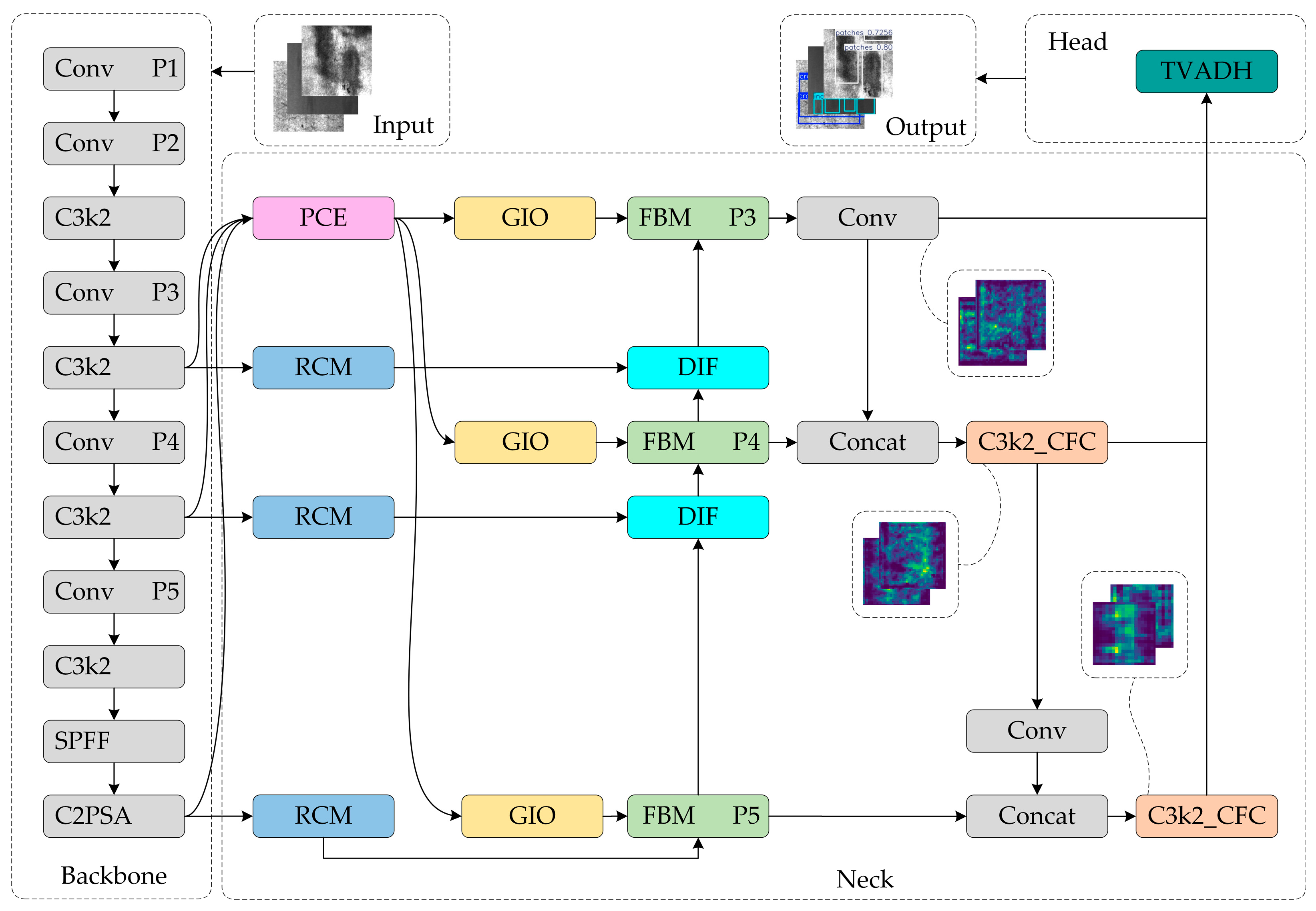
To enhance the recognition efficiency of the method in industrial blemish detection scenarios, this paper presents the efficiency of the CTL-YOLO detection technique in terms of resource utilization, based on the YOLO11n algorithm. The proposed method aims to maximize efficiency in detecting hot-rolled strip steel surface defects on terminal devices with limited computational power. First, this study proposes CGRCCFPN, a network for global feature fusion across multiple scales that combines the Rectangular Self-Calibration Module [22], Ca Former [23], and CGLU [24]. Secondly, this study proposes TVADH, a Variable Alignment Detection Head designed by referencing the concepts of Group Norm [25] and TOOD [26]. Finally, this study uses the LAMP [27] pruning algorithm to achieve global adaptive magnitude compression and simplification. An overview of the improved network configuration is presented in Figure 1.
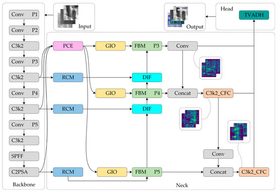
Figure 1.
CTL-YOLO network structure.
2.3. Context-Guided Reconstruction and Cascaded Cross Fusion Pyramid Network
Based on the feature fusion network’s performance in the hot-rolled strip steel surface defect detection tasks, where simple upsampling and concatenation operations are used to fuse feature maps, it lacks the dynamic modeling ability for contextual information of defects at different scales. The fixed structure of convolutional stacks struggles to adapt to the complex and varying defect morphology, and conventional pyramid structures tend to weaken shallow texture information during feature propagation. However, defect detection on hot-rolled strip steel surfaces heavily relies on pixel-level spatial features. To address this, this paper proposes a Neck network called the Context-Guided Reconstruction and Cascaded Cross Fusion Pyramid Network (CGRCCFPN). Its role is to aggregate global context through pyramid pooling, combine dynamic interpolation fusion mechanisms to enhance multi-scale feature representation capabilities, and embed a channel attention mechanism in convolutions. This allows for a collaborative optimization of local feature enhancement and global semantic guidance, effectively solving key issues such as multi-scale feature imbalance and high missed detection rates for small targets in hot-rolled strip steel surface defect detection.
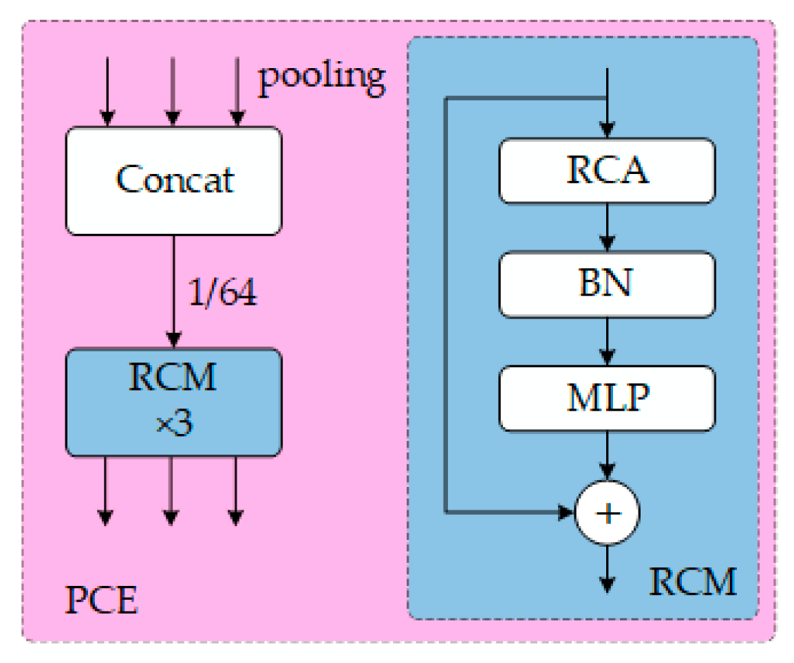
The output feature maps P3, P4, and P5 from the Backbone network are employed to process the multi-scale detail maps for CGRCCFPN. These feature maps undergo pyramid pooling aggregation via the Pyramid Context Extraction (PCE) module. Multi-scale pooling is applied to each level’s feature map, generating global context features. These features are then fused within a multi-scale context through cascading and 1 × 1 convolutions, represented as follows:
where represents the l-th level feature map output by the Backbone network (e.g., ), is the size of the pooling kernel (with values of 1 × 1, 3 × 3, or 5 × 5), and denotes the feature map obtained after performing adaptive average pooling on .
where Concat refers to concatenating multi-scale pooling results along the channel dimension, represents a 1 × 1 convolution (employed for reducing channels and feature fusion), and refers to the globally fused contextual features. This helps to effectively combine features from various layers, improving the model’s contextual awareness. Through the Rectangular Self-Calibration Module (RCM), depthwise separable convolution and spatial attention are applied to reconstruct features, represented as follows:
where refers to depthwise separable convolution, is a convolution (used for generating spatial attention weights), is the Sigmoid activation function, ⊗ denotes element-wise multiplication, and represents the enhanced regional contextual features. The RCM facilitates spatial feature reconstruction and the extraction of pyramid context. It captures global information along both the horizontal and vertical axes, while also acquiring axial context to effectively model the key rectangular regions. The workflow of the PCE and RCM modules is shown in Figure 2.

Figure 2.
PCE and RCM module structure.
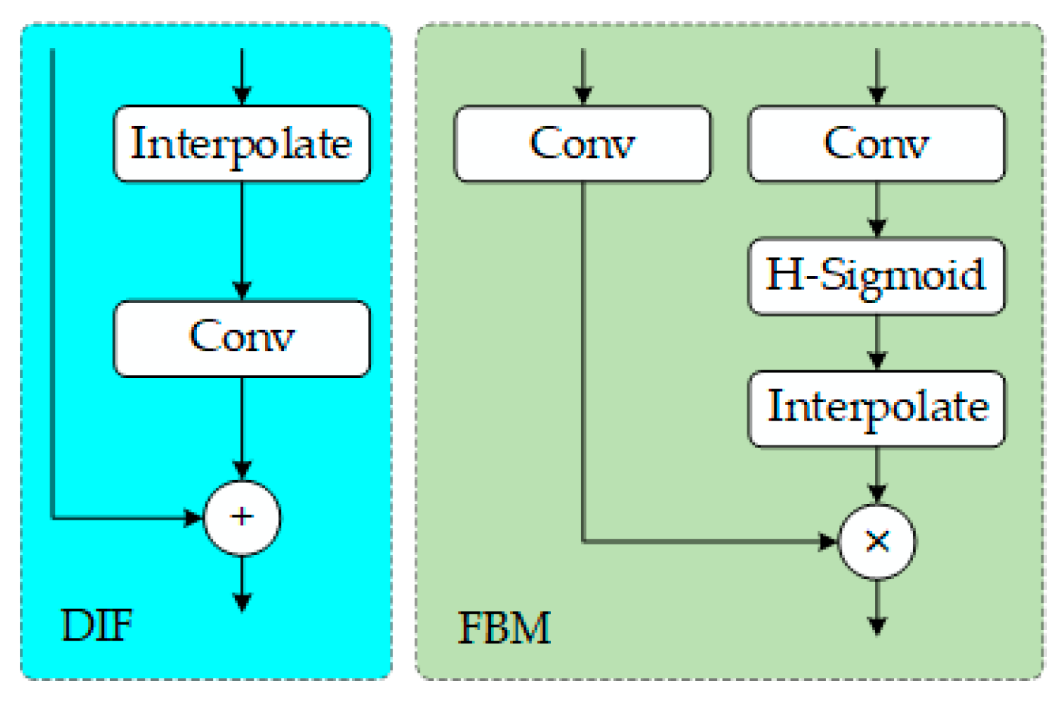
The Get Index Output (GIO) module separates the fused features into three hierarchical features, P3/8, P4/16, and P5/32, enabling feature layering, which makes the presentation more intuitive and facilitates code development. The FBM (Fuse Block Multi) performs a gated fusion of enhanced features from P5, P4, and P3 with the pyramid-extracted contextual features from P5, P4, and P3, as expressed by the following:
where represents high-level information, represents low-level information, is the convolution kernel for transforming low-level features, is the convolution kernel for transforming high-level features, is the Sigmoid activation function, UpSample refers to bilinear interpolation upsampling, ⊗ denotes element-wise multiplication, and is the fusion result. The Dynamic Interpolation Fusion (DIF) module adaptively adjusts the high-level semantic information and low-level detail information, as expressed by the following:
where represents the learnable upsampling kernel, is the scaling factor, and ⊕ denotes element-wise addition. The FBM and DIF are used for multi-scale information gathering. Through dynamic interpolation and multi-scale information gathering, the information enhances the model’s ability to represent multi-scale features and improves its ability to identify targets in complex backgrounds. The workflow is illustrated in Figure 3.
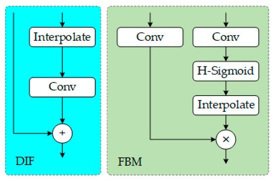
Figure 3.
DIF and FBM module structure.
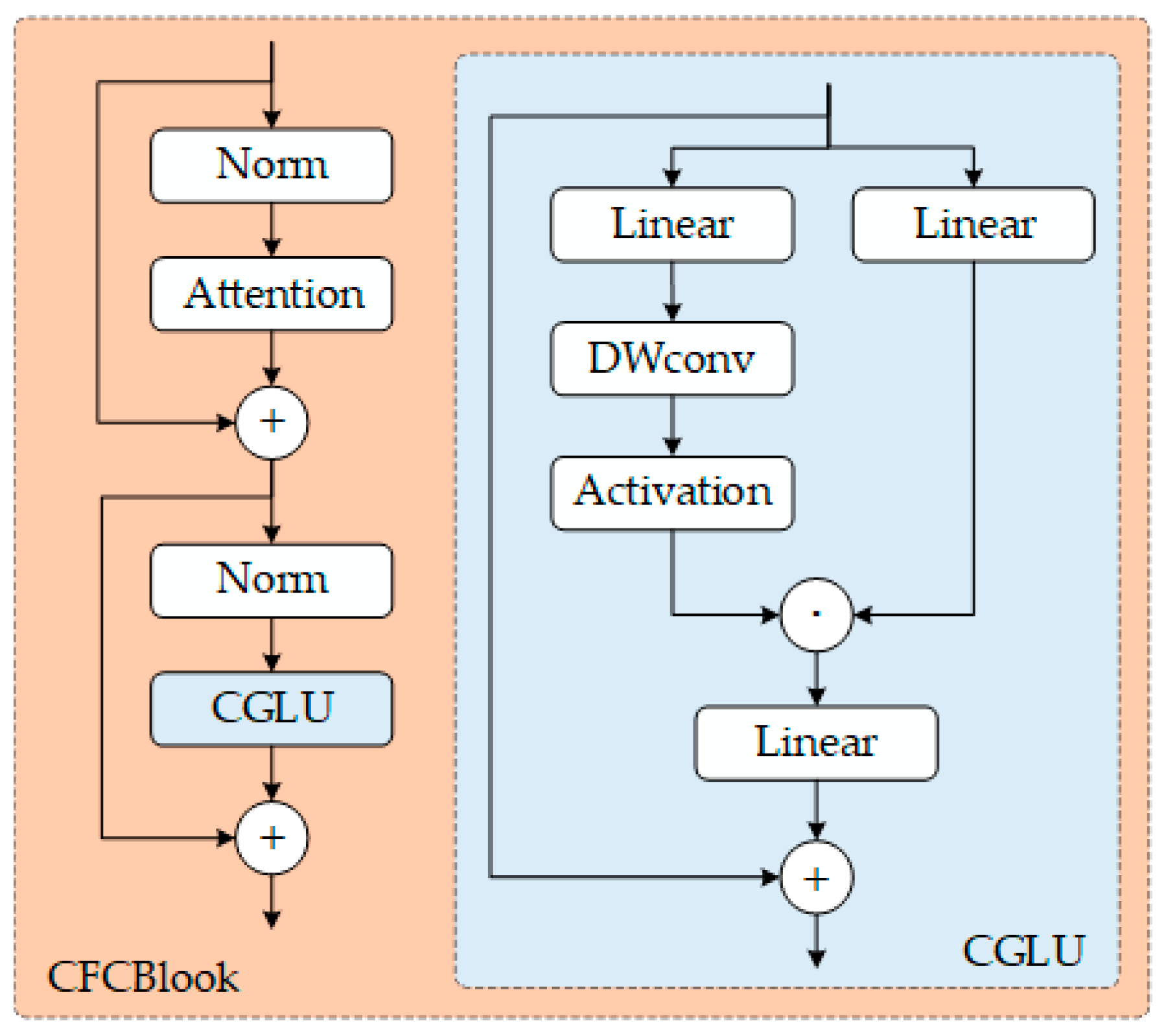
The input information for multi-scale convolution decomposition is processed through the C3k2 branch to complete the feature reorganization stage. The CaFormer is used for local–global attention interaction to achieve context aggregation, and the CGLU is employed for feature selection to complete the gated nonlinear transformation. The C3k2-CaFormer-CGLU (C3k2_CFC) module combines convolutional attention with gating mechanisms, as expressed by the following:
where represents the input feature map, CGLU refers to the Convolutional Gated Linear Unit, ⊗ denotes element-wise multiplication, DropPath is the Stochastic Depth technique, LayerNorm refers to Layer Normalization, and TokenMixer is the rectangular region attention mechanism based on CaFormer, as expressed by the following:
where represent the Query, Key, and Value matrices, respectively, where are learnable projection matrices, with representing the scaling factor dimension. denotes the rectangular mask, ⊗ denotes element-wise multiplication, and is the scaling factor. The C3k2_CFC module enhances feature discriminability. The C3k2_CFC module is obtained by replacing the Meta Former Block of C3k2 with the CFCBlook we developed. To effectively reduce computational and parameter complexity, the C3k2_CFC module is placed at locations with smaller feature map sizes to output the features required for the final identifying head. The workflow is illustrated in Figure 4.
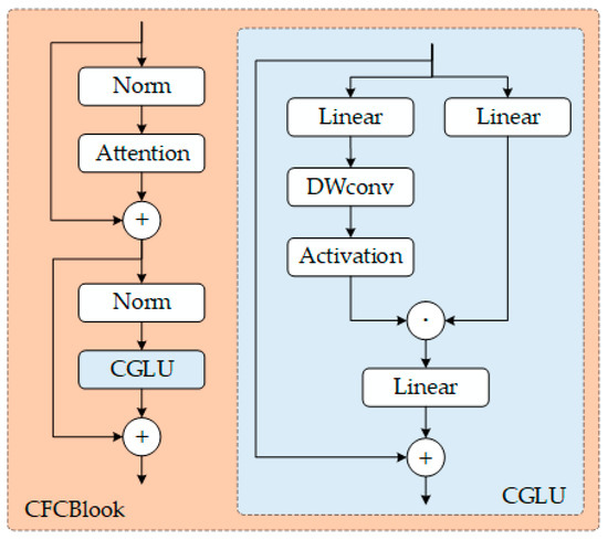
Figure 4.
CFCBlook module structure.
In summary, CGRCCFPN achieves efficient multi-scale information gathering and detail preservation in hot-rolled strip steel surface blemish detection through context-guided feature reconstruction and a lightweight attention mechanism. It adaptively adjusts the semantic weights of defects at different scales, enabling dynamic context awareness and enhanced feature discriminability. Testing on the NEU-DET dataset demonstrates that the algorithm surpasses the traditional Neck structures.
2.4. Task Variable Alignment Detection Head
Traditional detection heads adopt a parallel classification and regression branch design, and their feature fusion strategy lacks task-oriented guidance, which suppresses the discriminability of multi-scale defects. The fixed convolution kernels are unable to dynamically adapt to spatial shifts in intricate textured context, resulting in a decrease in localization accuracy. In the hot-rolled strip steel surface defect detection scenario, defects often exhibit characteristics such as varying scales, irregular shapes, and low contrast. To address this, this paper proposes a Head network called Task Variable Alignment Detection Head (TVADH), as shown in Figure 5.
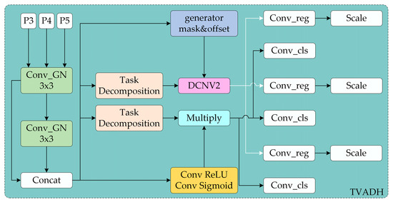
Figure 5.
TVADH network structure.
Two layers of lightweight Conv_GN (Group Normalization + Depthwise Separable Convolution) are used to collect basic information and output the information dimensions. This reduces the feature distribution shift caused by uneven lighting in industrial scenes, decreases noise interference in industrial images, and lowers computational complexity, thus meeting the real-time detection requirements. Multi-scale context information is preserved as shared feature extraction. The Task Decomposition module reorganizes features through channel attention, allowing the classification branch to focus on defect semantic information, while the regression branch learns spatial geometric features, achieving dual-path task decoupling and decomposition, as expressed by the following:
where represents the feature map, AvgPool refers to average pooling, CLSDecomp is classification decomposition, and REGDecomp is regression decomposition. In the regression branch, the Generator mask and offset uses a 3 × 3 convolution to generate the offset and modulation factor to predict the offset. DCNV2 [28] refers to the dynamic deformable convolution, which performs adaptive deformation feature alignment, as expressed by the following:
where represents the pixel coordinates on the feature map, is the offset of the sampling point relative to the center coordinate, is the predicted offset, is the spatial modulation factor, is the fixed convolution kernel weight, and is the aligned regression feature map. The regression branch enables the convolution kernel to adaptively deform to the local irregularities of the hot-rolled strip steel defect edges, improving the localization accuracy of small target defects. In the classification branch, Conv ReLU Conv Sigmoid uses two levels of 1 × 1 convolutions to compress the channels, and a 3 × 3 convolution generates the spatial probability map. Multiply is used to re-weight the features, with pixel-wise multiplication suppressing background noise. The spatial probability map highlights the defect regions and suppresses false positives caused by the surface texture. Finally, the independent channel attention modules, Conv_reg and Conv_cls, are used to decouple classification and regression features, alleviating task conflicts.
In summary, TVADH predicts the convolution kernel offsets based on feature content, and the variable adjustment of convolution sampling points can enhance the localization robustness of irregular defects. The entire process utilizes the shared convolution layer parameters for reuse, considerably lowering the params compared to traditional detection heads. Its performance on the NEU-DET dataset demonstrates excellent results in comparison with the conventional Head structures.
2.5. Layer-Adaptive Magnitude-Based Pruning
Deep neural networks commonly experience parameter superfluity and inefficient feature representation, which severely restricts the deployment performance of lightweight detection algorithm on weak computing power terminals. To address this, this study introduces the Layer-Adaptive Magnitude-Based Pruning (LAMP) [27] algorithm to optimize the proposed algorithm. LAMP establishes an inter-layer importance adaptive evaluation mechanism and uses dynamic thresholds to protect shallow, fine-grained information. This facilitates the precise pruning of the model parameters while preserving the ability to express key features, thereby solving the challenge of balancing computational efficiency and detection accuracy. Pruning refers to the use of the LAMP algorithm to prune the structurally improved YOLO model of redundant parameters.
The channel pruning strategy of LAMP is based on the core principle of achieving adaptive inter-layer sparsity allocation through weight magnitude analysis, rather than pruning the entire network uniformly. For a feedforward neural network with depth g, given the weight tensors of each layer , the algorithm first flattens the weights of each layer into one-dimensional vectors and arranges them in ascending order, ensuring that for indices , . The LAMP score for each weight is defined as follows:
where and are index values of the weights, and and represent the weight elements corresponding to indices and . This score establishes a relative evaluation system for weight importance through normalization. The numerator term characterizes the local importance of the target weight, while the denominator term quantifies the global influence of this weight within the layer. It is expressed by the following formula:
A larger weight magnitude corresponds to a higher LAMP score, which provides a theoretical basis for selecting the pruning threshold. By dynamically adjusting the sparsity thresholds of each layer, the algorithm systematically removes low-scoring connections until the desired global compression rate is achieved. Finally, the YOLO model, pruned of redundant parameters, usually requires fine-tuning to restore or improve the performance prior to pruning.
In summary, the LAMP algorithm introduced in this study adaptively evaluates important functions and protects key feature layers through a dynamic threshold mechanism. It significantly reduces the sophistication and data of the algorithm, innovatively addressing the model lightweighting challenge in industrial detection scenarios. Testing on the NEU-DET dataset demonstrates that its performance meets the dual requirements of efficient and precise defect detection for hot-rolled production lines.
3. Experiment
3.1. Dataset Description
In order to verify the effectiveness and the predictive ability of the unseen data of the proposed method, this study uses two popular public datasets, namely the NEU-DET [29] dataset for hot-rolled strip steel surface blemish detection and the GC10-DET [30] dataset. The two datasets are divided into training, validation, and test sets in an 8:1:1 ratio, which is a standard practice for dataset division in deep learning tasks.
3.1.1. NEU-DET
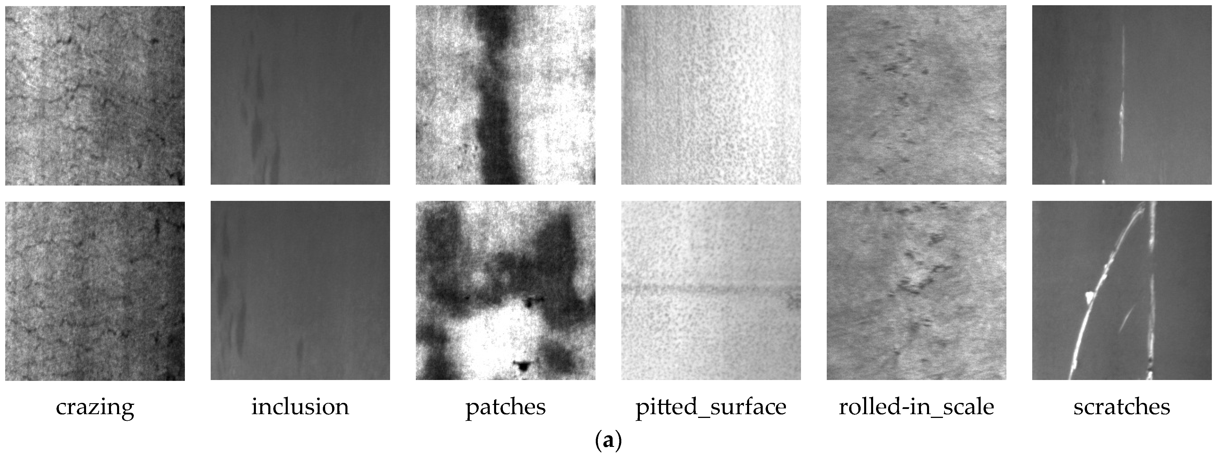
This study uses the NEU-DET dataset, which was collected and made publicly available by Professor Song Kechen’s team at Northeastern University. The dataset contains six types of defects specifically designed for steel surface defect detection, including six common industrial defects, with 300 images per category, totaling 1800 images. The categories are Scratches (Sc), Crazing (Cr), Pitted Surface (Ps), Inclusion (In), Patches (Pa), and Rolled in Scale (Rs), as shown in Figure 6. Each image in this dataset contains only one defect instance, which simplifies the detection task and is suitable for algorithm validation.
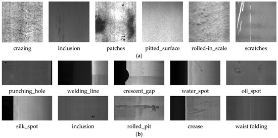
Figure 6.
(a) NEU-DET dataset; (b) GC10-DET dataset.
3.1.2. GC10-DET
This study uses the GC10-DET dataset, which was collected from real-world industrial environments and focuses on steel surface defects. It includes 10 common types of metal surface defects, with a total of approximately 3600 images. The defects are categorized as follows: punching hole (Pu), welding line (Wl), crescent gap (Cg), water spot (Ws), oil spot (Os), silk spot (Ss), inclusion (In), rolled pit (Rp), crease (Cr), and waist folding (Wf), as shown in Figure 6. This dataset covers a wide range of industrial defect types and is suitable for target detection and classification research in complex scenarios.
3.2. Experimental Environment
The experiments were performed on an online server with the following configuration: Ubuntu 22.04 operating system, AMD EPYC 7352 processor, NVIDIA GeForce RTX 4090 24 GB GPU, 124 GB RAM, a 100 GB hard drive, PyTorch 2.3.0 deep learning framework, CUDA 12.1 parallel computing architecture, Python 3.10.15 programming language, and Ultralytics YOLO v8.3.9. The model training parameters are illustrated in Table 1.

Table 1.
The model training parameters.
3.3. Experimental Metrics
Precision (P) is the proportion of true positive samples among the samples predicted as positive. The formula is as follows:
where TP represents true positives, and FP represents false positives. This metric is used to evaluate the accuracy of the model’s predictions.
Recall (R) is the proportion of true positive samples among the samples that are actually positive. The formula is as follows:
where FN represents false negatives.
mAP50 refers to the mean Average Precision (AP) at an IoU threshold of 0.5. AP is the area under the precision–recall curve for each class. The mean AP across all classes is then calculated to obtain mAP50. The formula is as follows:
This metric is a core indicator in object detection, reflecting the general effectiveness of the algorithm under a relaxed IoU requirement.
mAP50:95 is the mean Average Precision (mAP) calculated across IoU thresholds ranging from 0.5 to 0.95, with the mAP at each threshold being averaged. It is used to assess the robustness of the model under varying localization accuracies.
Giga Floating-point Operations Per Second (GFLOPs) refers to the number of floating-point operations required for a single forward inference of the model, measured in billions. The formula is as follows:
where represents the number of input channels, is the kernel size, and represent the width and height of the output feature map, respectively, and represents the number of output channels. The FLOPs are divided by to obtain the GFLOPs. This metric is used to measure computational complexity, with higher values indicating greater hardware computational power requirements.
Frames Per Second (FPS) refers to the number of images the model can process per second. This metric directly reflects real-time performance, with higher FPS indicating lower latency.
Params refers to the total number of trainable parameters in the model, measured in millions. A larger params imply higher algorithm complexity, requiring more storage and occupying more memory.
The size refers to the disk space occupied by the model after being saved as a file.
3.4. Experimental Detail
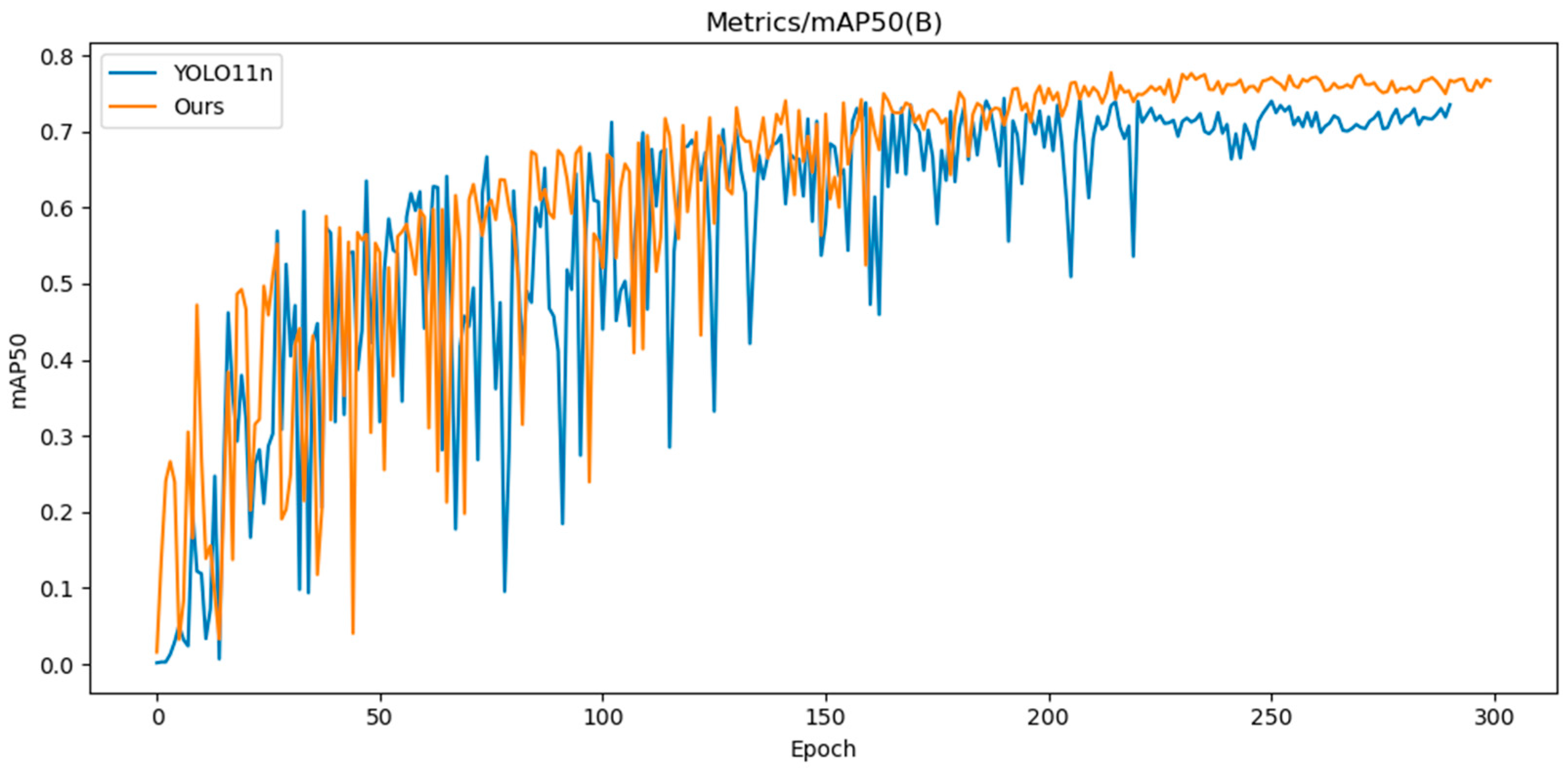
The training iteration graph, P-R curve, and confusion matrix for YOLO11n and CTL-YOLO, obtained based on the NEU-DET, are illustrated in Figure 7, Figure 8, Figure 9, respectively.
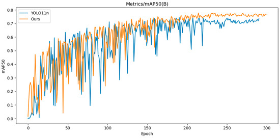
Figure 7.
YOLO11n and CTL-YOLO training iteration diagram.
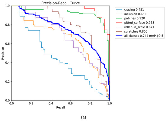
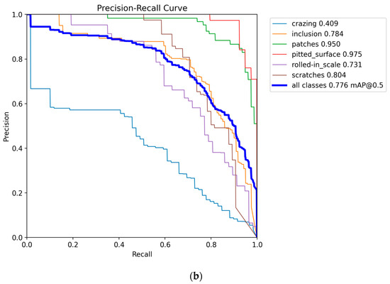
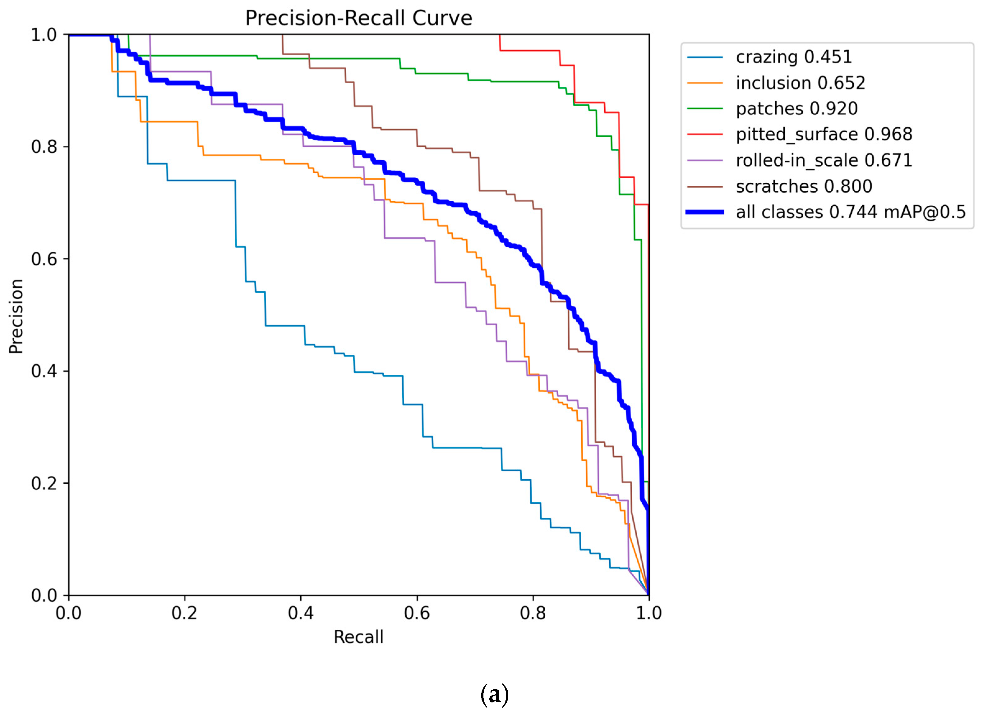
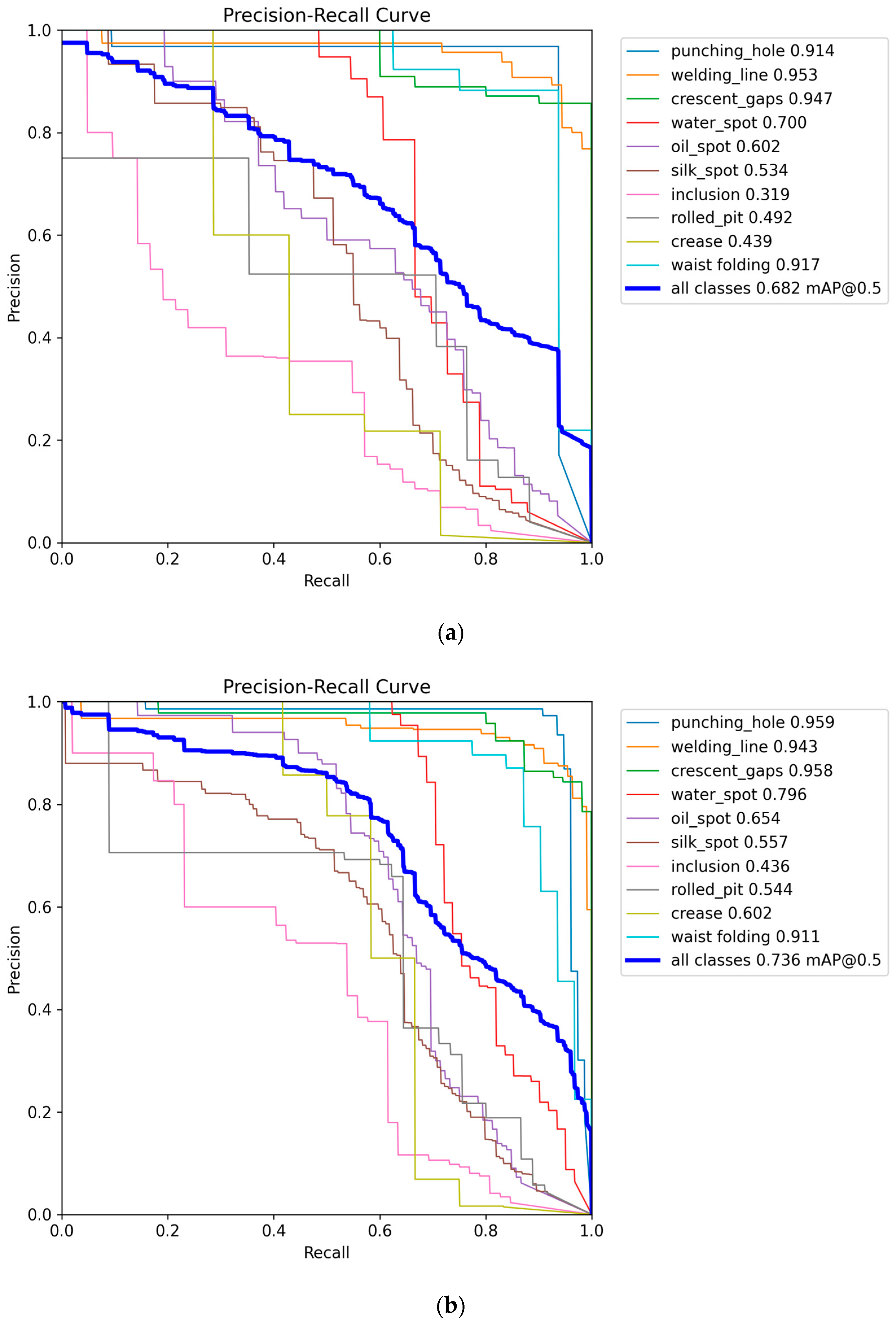
Figure 8.
(a) YOLO11n P-R curve; (b) CTL-YOLO P-R curve.

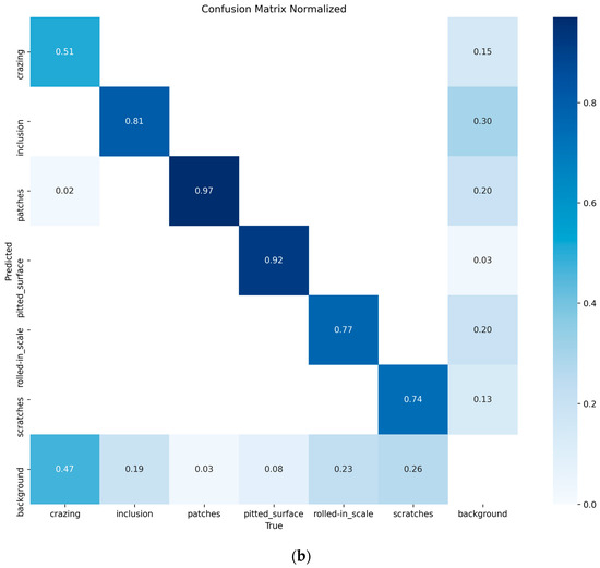
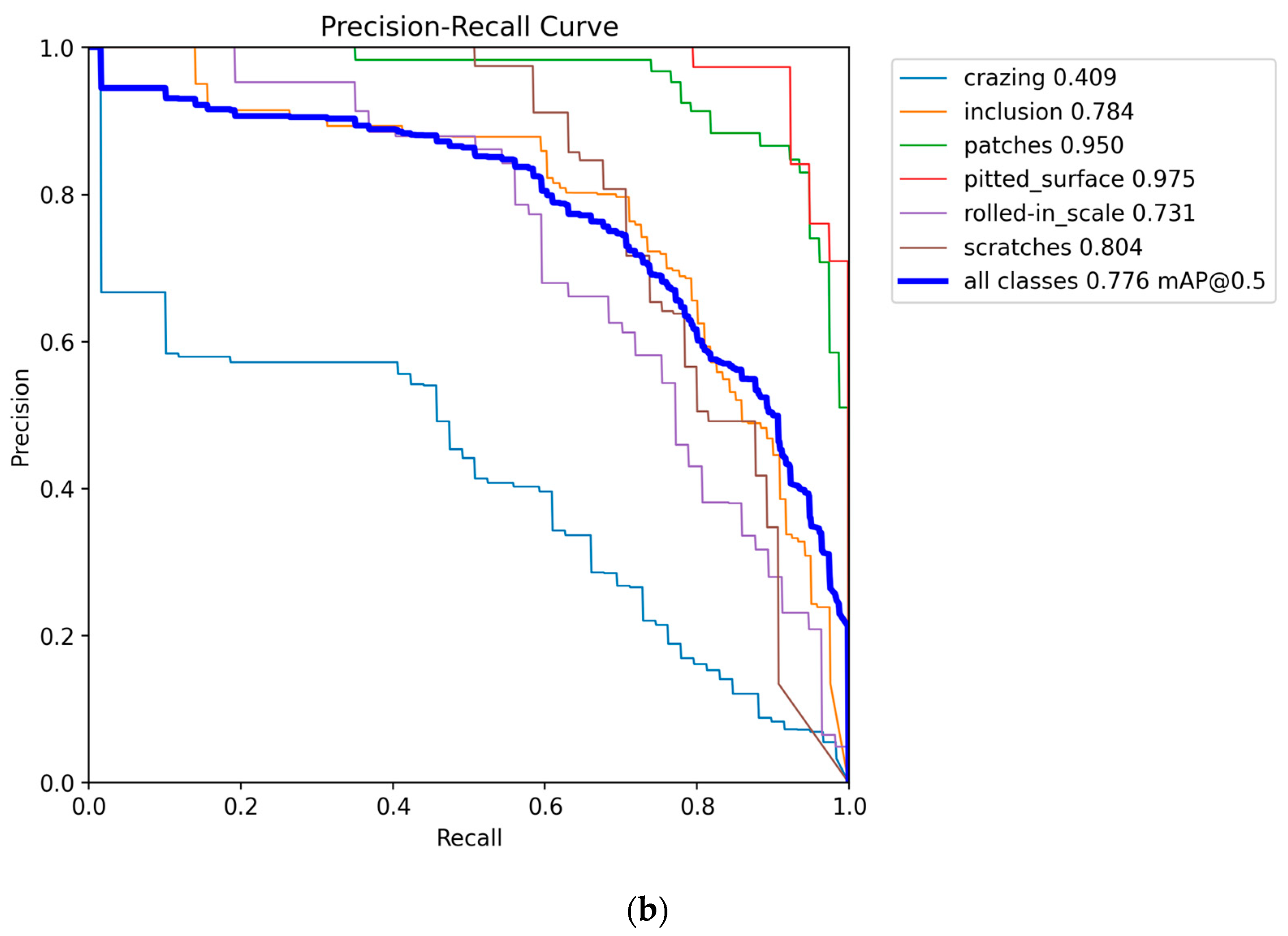
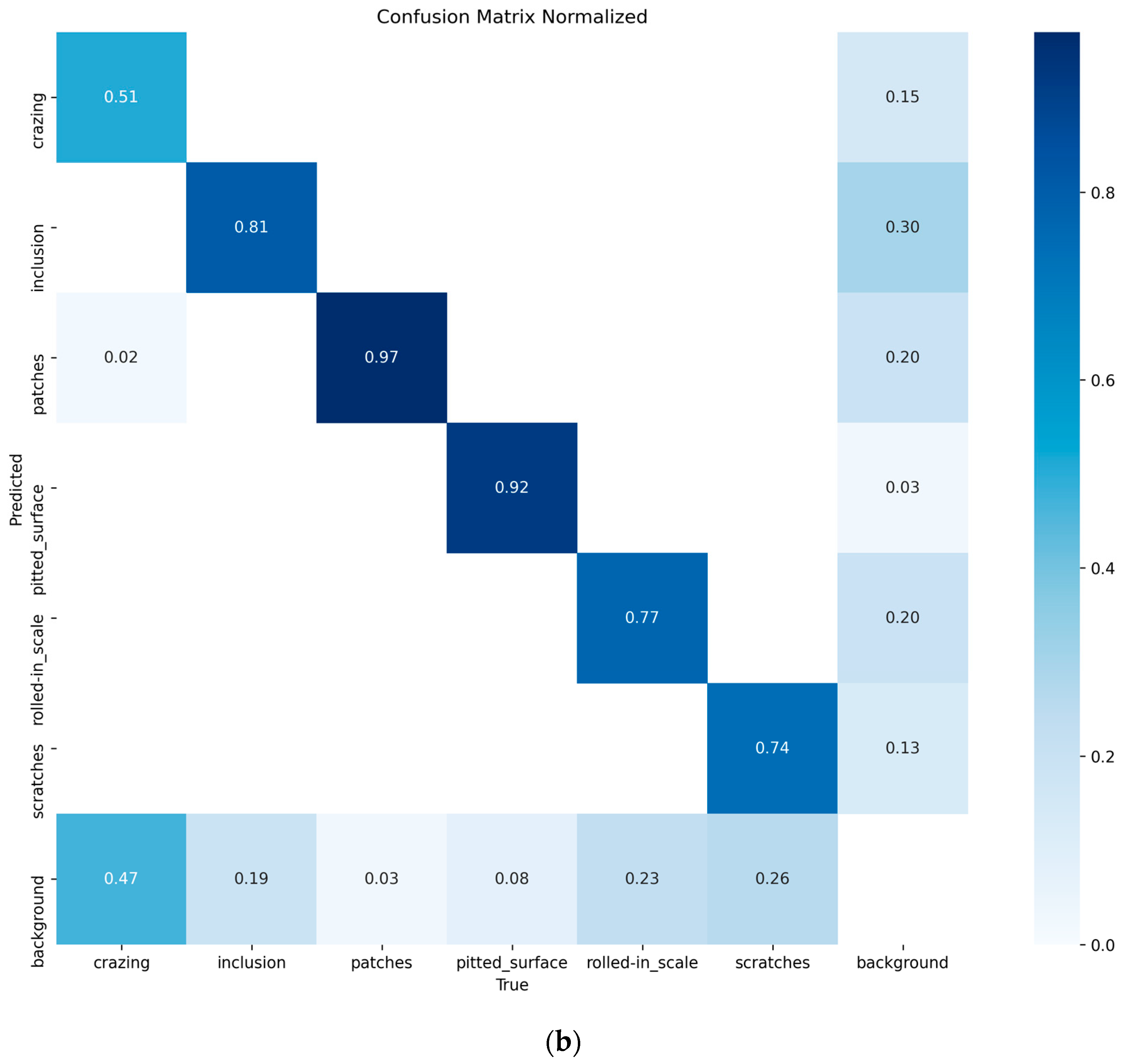
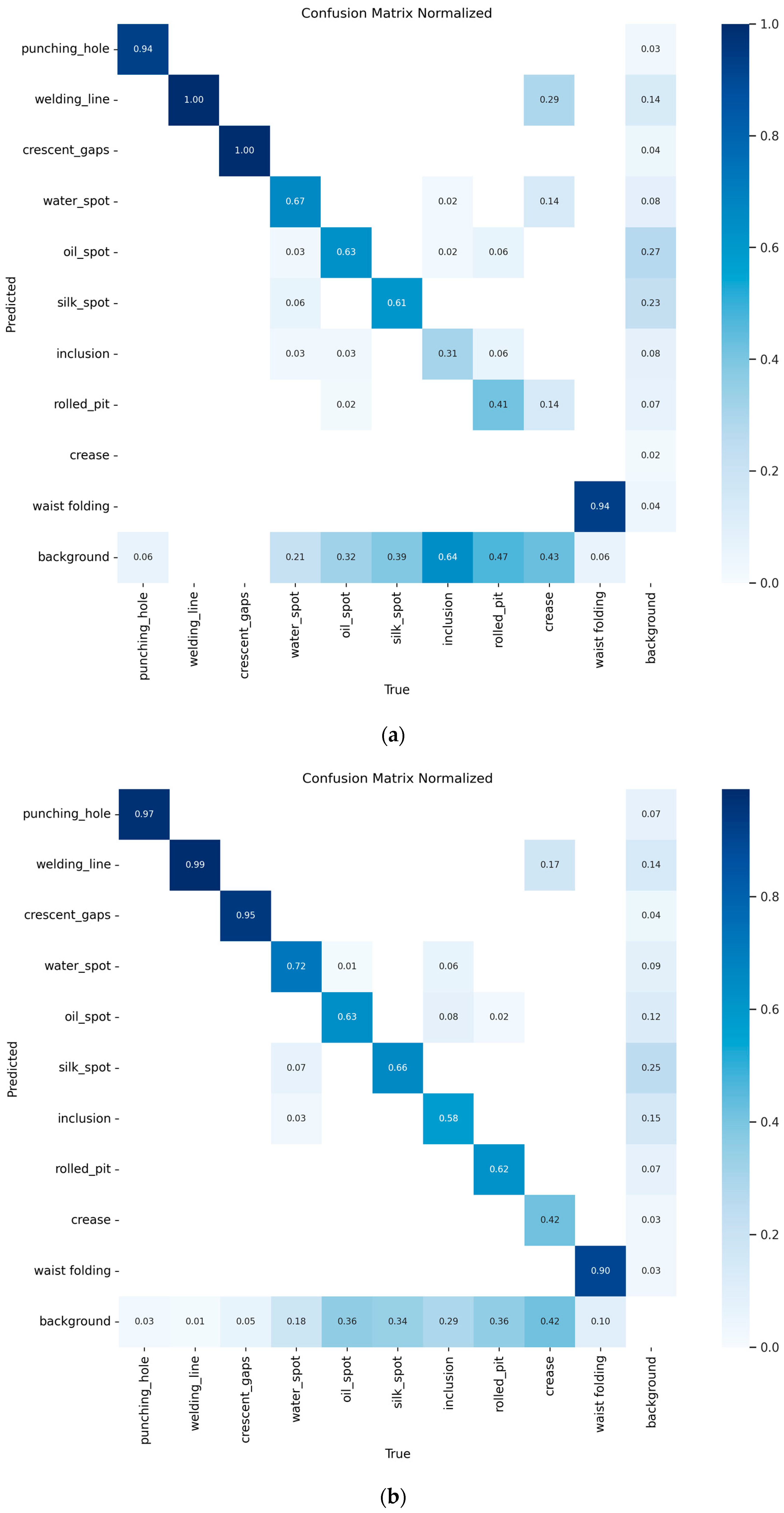
Figure 9.
(a) YOLO11n confusion matrix; (b) CTL-YOLO confusion matrix.
Based on the above results, it is evident that the precision of CTL-YOLO is significantly higher than that of the original YOLO11n algorithm, allowing for more accurate identification of the various defect types. From the training process, the precision curve of the original YOLO11n algorithm exhibits significant fluctuations, indicating poor stability. In contrast, CTL-YOLO stabilizes and gradually converges around the 230th iteration, demonstrating a better fitting performance. Although the mAP50 value for Cr slightly decreased, the mAP50 values for other defect types significantly improved. Furthermore, the accuracy of the correct predictions for Cr increased, and the correlation along the diagonal of the confusion matrix for other defect categories notably improved. This proves that the enhanced model meets the demands for defect detection in practical applications.
4. Results and Discussion
4.1. Superiority Verification
To test the feasibility of developing algorithms, a comparison was conducted using the NEU-DET among the YOLO11n baseline algorithm, current mainstream Neck networks, Head networks, and our developed network. Additionally, the optimal pruning rate for the pruning algorithm was determined. The experimental results are as follows, with the optimal values emphasized in bold.
4.1.1. Comparison of Neck Networks
To test the feasibility of CGRCCFPN, the outcomes of goldyolo-asf [31,32], EMBSFPN [33,34,35], Context Guide FPN (CGF) [36], and FDPN-DASI [37] applied to the same baseline model were compared, as indicated in Table 2. The experimental data indicate that the CGRCCFPN network demonstrates superiority across multiple key metrics, with an accuracy of 73.3%, which is an improvement of 6.8 percentage points over the baseline model. In terms of the overall performance metric, mAP50, CGRCCFPN leads all comparison methods with 76.0%, which is an improvement of 1.6 percentage points over the baseline model, while maintaining a recall rate of 70.6% and achieving performance balance. Although the computational metric, GFLOPs, and the number of parameters slightly increased compared to the baseline algorithm, the computational efficiency remains superior when compared to similar improvement methods like goldyolo-asf. These experimental results indicate that the proposed CGRCCFPN network achieves excellent functioning in terms of both accuracy and precision.
Table 2.
Comparison results of Neck networks.
4.1.2. Comparison of Head Networks
To test the feasibility of TVADH, Table 3 presents a comparison of the performances by LSCD [25,26], dyhead [38], EfficientHead [39], and SEAMHead [40] when applied to the same baseline model. The experimental data indicate that the TVADH network demonstrates significant improvements across multiple key metrics. It achieves an mAP50 score of 75.5%, which is an improvement of 1.1 percentage points over the baseline model, while surpassing the existing mainstream Head structures. Although the computational load is slightly higher than the baseline model, it remains at a reasonable level when compared to dyhead, which shows a similar improvement in accuracy. In terms of precision–recall balance, the algorithm has the best overall performance, with 67.7% precision and 73.0% recall, compared to the baseline model’s 66.5% P% and 72.6% R%, demonstrating better detection stability. Notably, the model’s parameter count is reduced to 2.20 M, a 14.7% decrease from the baseline model, making it the most parameter-efficient structure among the methods listed in the table. This indicates that the proposed TVADH network achieves a good balance between accuracy improvement and model lightweighting.
Table 3.
Comparison results of Head network.
4.1.3. Prune Study
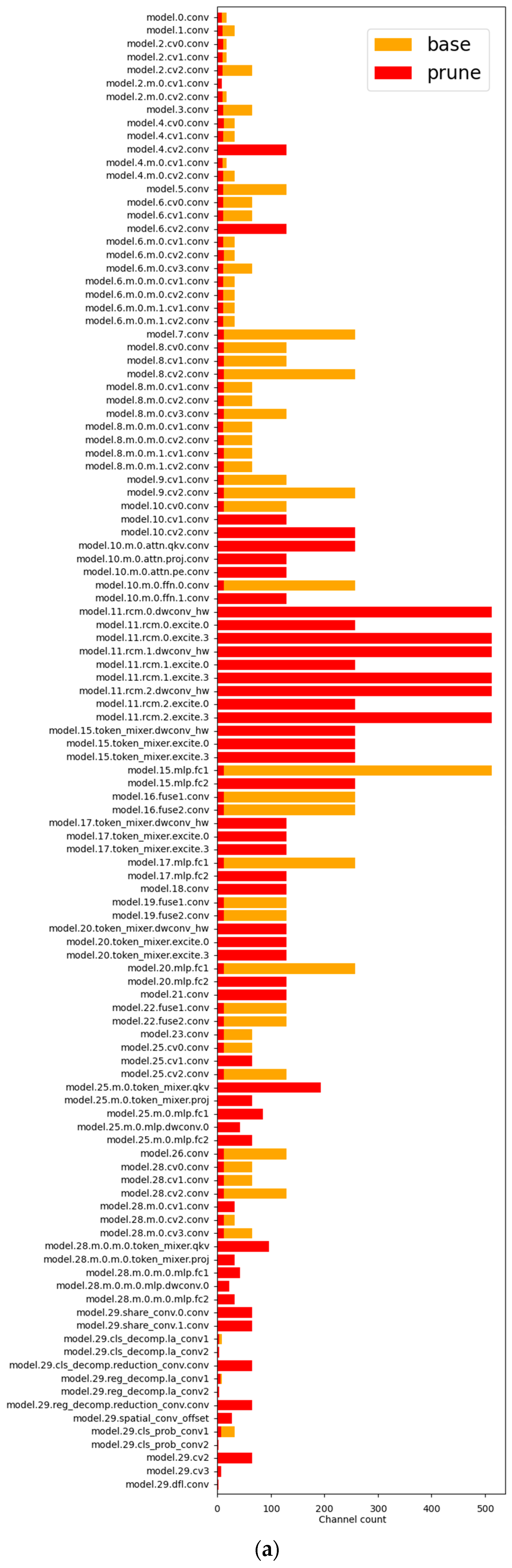
To test the feasibility of the pruning strategy, this study conducted comparative experiments with different pruning rates, ranging from 3.5× to 5.0×. The final comparison is presented in Table 4. The data indicate that, as the pruning rate increases, the model’s GFLOPs, params, and size all show a significant decreasing trend. When the pruning rate reaches 4.0×, the model’s GFLOPs decrease to 2.0, only 24.3% of the original value, representing a 75.6% reduction; the parameter count is compressed to 0.40 M, just 17.7% of the original, a reduction of 82.3%; and the model size shrinks to 1.2 MB, only 21.1% of the original, a reduction of 78.9%. At the same time, the mAP50 detection accuracy remains fully consistent with the baseline model. It is noteworthy that when the pruning rate exceeds 4.0×, the model performance significantly degrades. A 4.5× pruning rate results in a 7.4 percentage point decrease in mAP50, while a 5.0× pruning rate causes an 11.5 percentage point performance loss, indicating that excessive pruning severely disrupts the model’s performance. Based on the balance between accuracy and efficiency, the experiment ultimately selects Exp2 4.0× as the optimal pruning configuration. The channel comparison chart, computational flow diagram, computational load comparison chart, and parameter comparison chart are shown in Figure 10. This configuration successfully constructs a lightweight network structure with computational resource requirements only 24.3% those of the original model.
Table 4.
Comparison of different pruning rates.
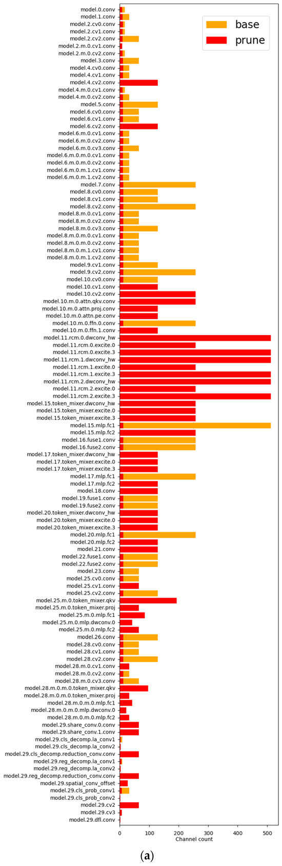
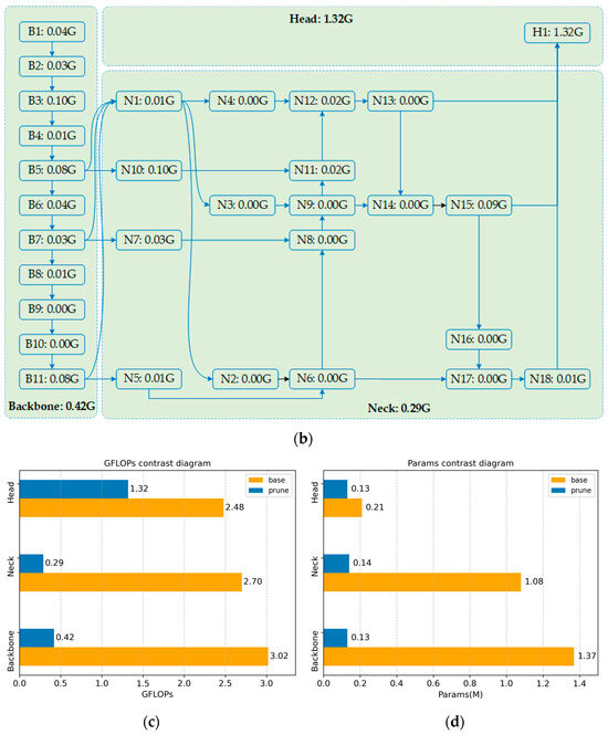
Figure 10.
(a) Channel contrast diagram; (b) Calculation flow chart; (c) GFLOPs contrast diagram; (d) Params contrast diagram.
4.2. Performance Comparisons
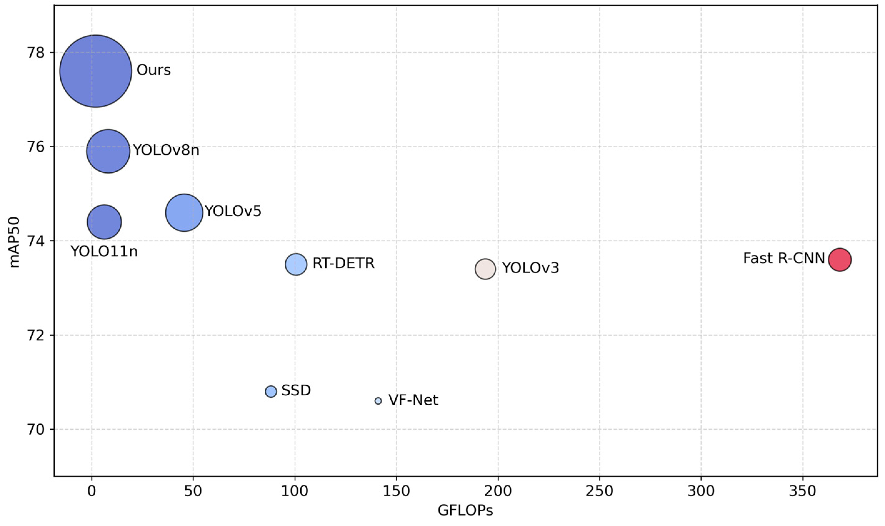
To test the feasibility of the CTL-YOLO algorithm, this study compared the experimental results of CTL-YOLO with the other mainstream algorithms on the NEU-DET, as illustrated in Table 5 and Table 6 and Figure 11. The CTL-YOLO algorithm has made breakthrough progress in detecting the unique defects Pa, Ps, and Rs on hot-rolled strip steel, achieving improvements of 3.0%, 0.7%, and 6.0% over YOLO11n, respectively. The mAP50 reached 77.6%, which is an improvement of 1.7 percentage points over the current best YOLOv8n. The mAP50:95 metric reached 44.0%, significantly outperforming YOLO11n’s 40.6%, demonstrating the improved algorithm’s enhanced multi-scale defect detection capability in complex backgrounds. The GFLOPs decreased to 2.0, only 31.7% of YOLO11n’s value, making it the algorithm with the lowest GFLOPs among the mainstream algorithms. The params were compressed to 0.4 M, a reduction of 84.5% compared to YOLO11n, and the size was reduced to 1.2 MB, meeting industrial embedded deployment standards. Despite maintaining high accuracy, the FPS reached 416.7 frames per second, which, although slightly lower than YOLO11n, still meets the real-time detection requirements. Memory usage is only 1/24 that of RT-DETR, and the computational energy consumption is equivalent to just 4.4% that of YOLOv5. Compared to the other lightweight algorithms of similar type, CTL-YOLO maintains the real-time advantages of the YOLO series while reducing the algorithm size by 78.2% compared to YOLO11n. The effectiveness of the enhanced model in the hot-rolled strip steel surface blemish detection task showed significant improvements. By optimizing accuracy, efficiency, and resource consumption in coordination, it addressed the “accuracy–computation” trade-off issue faced by traditional algorithms in complex industrial scenarios, offering a new technical solution for intelligent quality inspection in the steel industry.
Table 5.
Comparison results of different defects.
Table 6.
Comparison results of different algorithms.
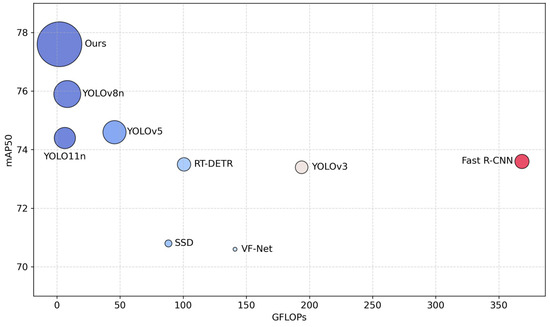
Figure 11.
Main comparisons of different algorithms.
4.3. Ablation Study
To test the feasibility of the changes in the CTL-YOLO algorithm, ablation experiments were performed on different improvement strategies, using YOLO11n as the baseline model on the NEU-DET dataset; the experimental outcomes are shown in Table 7. YOLO11n achieved a baseline performance of 74.4% mAP50 and 40.6% mAP50:95, with an inference speed of 769.2 FPS, demonstrating good real-time detection capability. When CGRCCFPN was introduced, the model showed improvements of 6.8 percentage points in precision (P) and 1.6 percentage points in mAP50, but the GFLOPs increased to 8.4, resulting in a reduction in FPS. The application of TVADH allowed the model to maintain high P, R, and mAP50 values while reducing the parameter count by 14.7%. The combined use of CGRCCFPN and TVADH exhibited significant synergistic effects, with the mAP50:95 metric increasing by 4.8 percentage points to 45.4%. Additionally, the shared parameter mechanism reduced the GFLOPs to 8.2, 2.4 lower than when using CGRCCFPN alone. Finally, after introducing LAMP, the model maintained a 77.6% mAP50 while drastically reducing computational complexity by 75.6%, lowering GFLOPs to 2.0, reducing the parameter count by 84.5% to 0.40 M, and compressing the model size by 78.9% to 1.2 MB. The FPS reached 416.7, achieving the best balance between identification accuracy and algorithm lightweighting while maintaining real-time performance. These experimental outcomes verify the availability of each innovative part in enhancing information representation, reducing redundancy, and optimizing the model architecture.
Table 7.
Results of ablation experiment.
4.4. Visualization Chart
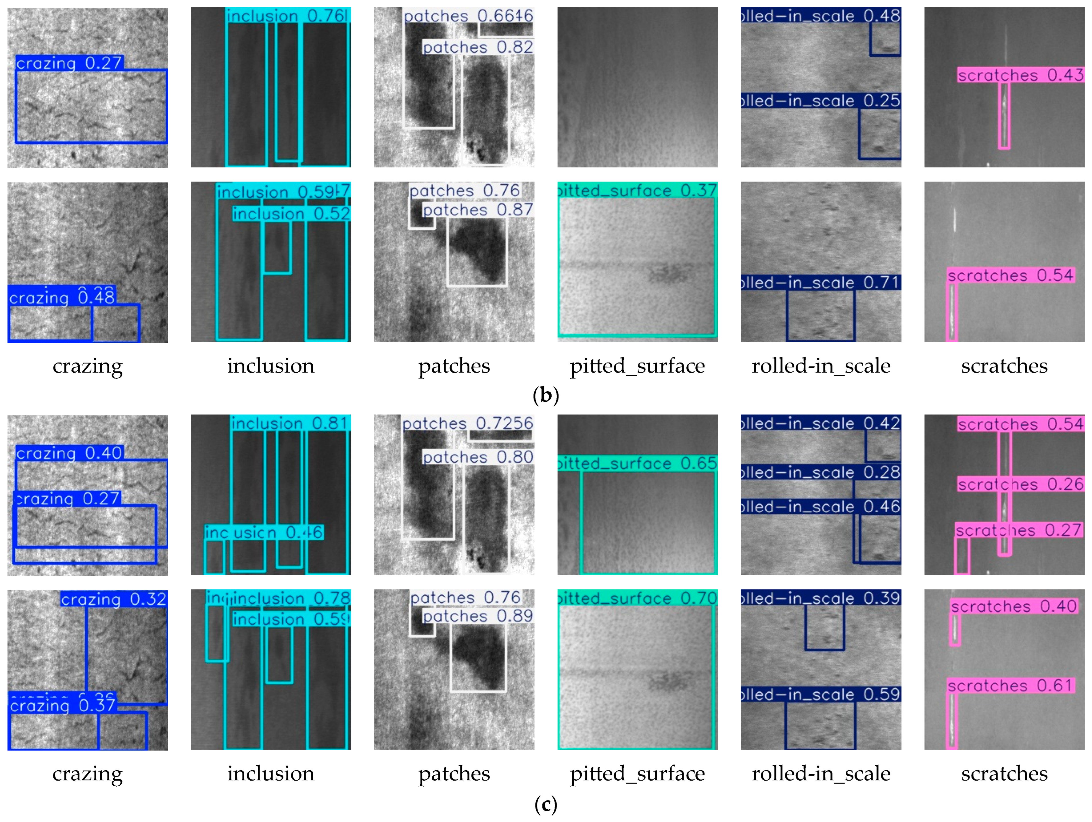
To visually demonstrate the identification capability of the YOLO11n and CTL-YOLO algorithms, a visualization was performed on the NEU-DET dataset, including prediction results and heatmaps, as shown in Figure 12 and Figure 13. Overall, CTL-YOLO exhibits a lower false negative rate, more accurate location identification, and more precise prediction results.
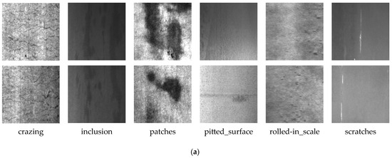

Figure 12.
(a) Original image; (b) YOLO11 recognition result; (c) CTL-YOLO11 recognition result.

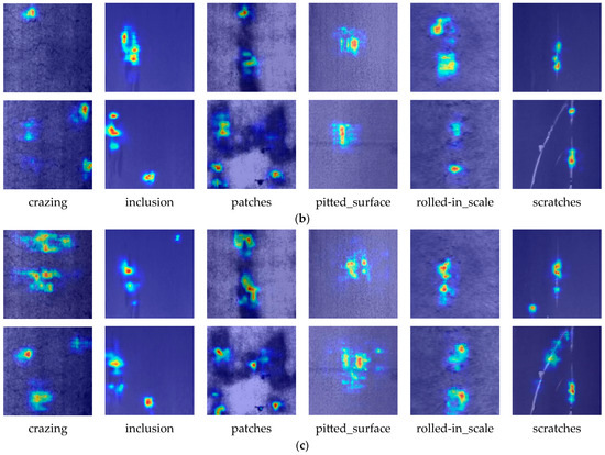
Figure 13.
(a) Original image; (b) YOLO11 heat map; (c) CTL-YOLO11 heat map.
4.5. Generalization Verification
To confirm the generalization ability of the CTL-YOLO, a multi-dimensional comparative experiment was performed on the GC10-DET dataset. The P-R curves of YOLO11n and CTL-YOLO are illustrated in Figure 14, and the confusion matrix is shown in Figure 15. The comparison results of CTL-YOLO with the other mainstream algorithms are illustrated in Table 8 and Table 9. The final test shows that the CTL-YOLO algorithm achieves optimal values for Rp and Cr defect recognition, with performance scores of 54.4% and 60.2%, respectively, outperforming all the comparison algorithms. Compared to the baseline model YOLO11n, Rp and Cr improved by 5.2% and 16.3%, indicating significantly enhanced detection capabilities for fine defects. Although the performance on the Wl defects is comparable to VF-Net and slightly lower than YOLOv8n on the Ws defects, the method in this paper shows a balanced performance overall. CTL-YOLO achieves the best overall capacity, with 74.5% precision and 71.9% recall, leading to the highest mAP50 (73.6%) and mAP50:95 (37.8%) values. Compared to the second-best model, RT-DETR-R18, the mAP50 improved by 2.0%, while the parameter count was reduced by 95.3%. The model demonstrates outstanding computational efficiency, requiring only 4.1 GFLOPs and achieving an inference speed of 555.6 FPS, 3.2 times faster than YOLOv5 s, while maintaining higher accuracy. The model’s parameter count is only 0.94 M, and its storage size is 2.2 MB, which is a 63.5% reduction in parameters compared to YOLO11n, with a 5.4% improvement in mAP50. These results show that the improved network architecture validly balances recognition accuracy and computational efficiency, with a significant reduction in algorithm complexity while achieving improved performance. The CTL-YOLO algorithm exhibits excellent generalization ability in the hot-rolled strip steel surface blemish detection task.
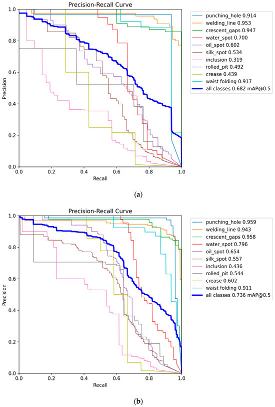
Figure 14.
(a) YOLO11n P-R curve on GC10-DET; (b) CTL-YOLO P-R curve on GC10-DET.
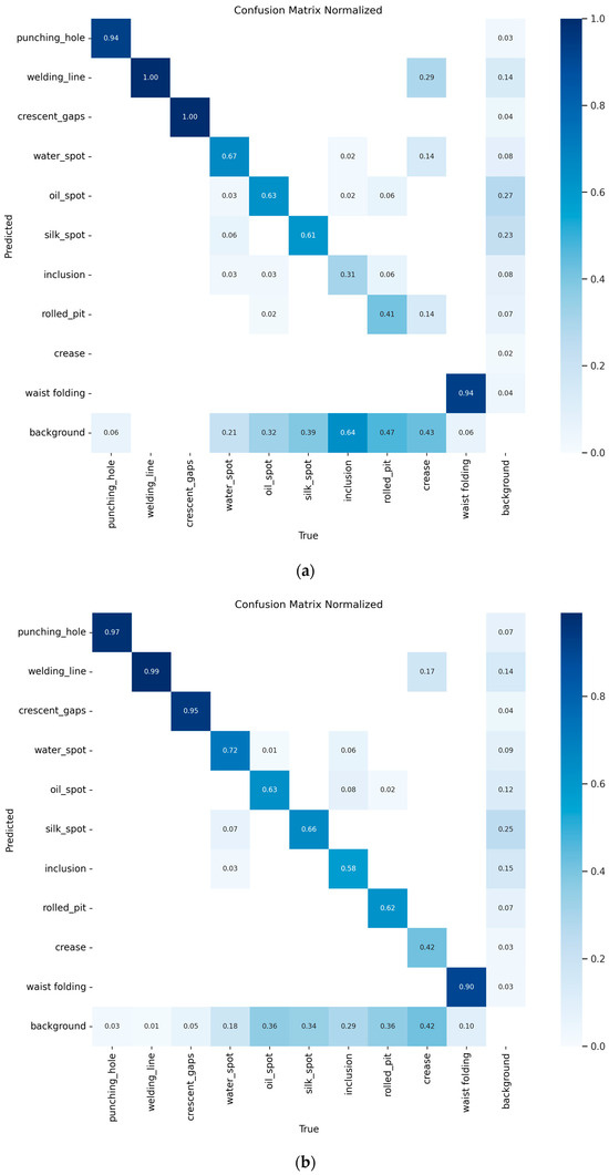
Figure 15.
(a) YOLO11n confusion matrix on GC10-DET; (b) CTL-YOLO confusion matrix on GC10-DET.
Table 8.
Comparison results of different defects on GC10-DET.
Table 9.
Comparison results of different algorithms on GC10-DET.
5. Conclusions
This study proposed applying the CTL-YOLO detection algorithm on the NEU-DET and GC10-DET datasets to explore the balance between computational efficiency and detection accuracy in hot-rolled strip steel surface defect detection. This research is a valuable supplement to the existing work, addressing gaps in the current studies and providing the necessary references for the steel industry. First, we explored the relationships among the Neck structure of YOLO11, multi-scale information fusion, and small target recognition. We proposed the CGRCCFPN feature fusion network, which achieved a more efficient fusion of multi-scale information, as well as better preservation of details. Next, we investigated the strategy of information sharing between the classification and regression branches in the Head structure. We introduced the TVADH network, which enabled shared convolutional layer parameter reuse between classification and regression, enhancing defect detection in complex backgrounds. Lastly, we applied the LAMP algorithm to prune redundant parameters of the YOLO model, decreasing the model’s computational and parameter, ensuring efficient operation even in weak computing devices. The experimental results showed that on the NEU-DET and GC10-DET datasets, CTL-YOLO achieved mAP50 values of 77.6% and 73.6%, separately, improving by 3.2 and 5.4 percentage points compared to YOLO11n. The GFLOPs were reduced to 2.0 and 4.1, which was a decrease of 68.3% and 34.9%, respectively. Params were reduced to 0.40 M and 0.94 M, which was a reduction of 84.5% and 63.6%, significantly outperforming the other tested models, especially in balancing computational efficiency and detection accuracy. The model size was reduced to 1.2 MB, meeting industrial embedded deployment standards. Of course, this study has some limitations, e.g., the FPS level is below that of the baseline algorithm. However, it still meets the real-time identification needs in industrial applications. In the future, we plan to combine knowledge distillation and quantization techniques to further compress the model size while ensuring its inference ability and generalization capability. Additionally, we will explore the applicability of different pruning methods on various neural network architectures to optimize deep learning models for more practical application scenarios.
Author Contributions
Conceptualization, N.M. and W.S.; methodology, W.S.; data curation, N.M.; writing—original draft preparation, W.S. and S.Y.; writing—review and editing, L.C. and S.T.; visualization, W.S. and Y.L. All authors have read and agreed to the published version of the manuscript.
Funding
This research received no external funding.
Data Availability Statement
The data presented in this study are available on request from the corresponding author.
Conflicts of Interest
The authors declare no conflicts of interest.
References
- Zhang, Y.; Zhang, H.; Huang, Q.; Han, Y.; Zhao, M. DsP-YOLO: An anchor-free network with DsPAN for small object detection of multiscale defects. Expert. Syst. Appl. 2024, 241, 122669. [Google Scholar] [CrossRef]
- Zhang, D.; Hao, X.; Wang, D.; Qin, C.; Zhao, B.; Liang, L.; Liu, W. An efficient lightweight convolutional neural network for industrial surface defect detection. Artif. Intell. Rev. 2023, 56, 10651–10677. [Google Scholar] [CrossRef]
- Zhang, J.; Li, Y.; Xiao, W.; Zhang, Z. Non-iterative and fast deep learning: Multilayer extreme learning machines. J. Frankl. Inst. 2020, 357, 8925–8955. [Google Scholar] [CrossRef]
- Tao, X.; Hou, W.; Xu, D. Review of Surface Defect Detection Methods Based on Deep Learning. Acta Autom. Sin. 2021, 47, 1017–1034. [Google Scholar]
- Ren, S.; He, K.; Girshick, R.; Sun, J. Faster r-cnn: Towards real-time object detection with region proposal networks. Adv. Neural Inf. Process. Syst. 2015, 28, 1137–1149. [Google Scholar] [CrossRef]
- Redmon, J.; Divvala, S.; Girshick, R.; Farhadi, A. You only look once: Unified, real-time object detection. In Proceedings of the IEEE Conference on Computer Vision and Pattern Recognition, Las Vegas, NV, USA, 27–30 June 2016; pp. 779–788. [Google Scholar]
- Liu, W.; Anguelov, D.; Erhan, D.; Szegedy, C.; Reed, S.; Fu, C.Y.; Berg, A.C. Ssd: Single shot multibox detector. In Proceedings of the Computer Vision–ECCV 2016: 14th European Conference, Amsterdam, The Netherlands, 11–14 October 2016; Proceedings, Part I 14. Springer: Berlin/Heidelberg, Germany, 2016; pp. 21–37. [Google Scholar]
- Zhong, H.; Fu, D.; Xiao, L.; Zhao, F.; Liu, J.; Hu, Y.; Wu, B. STFE-Net: A multi-stage approach to enhance statistical texture feature for defect detection on metal surfaces. Adv. Eng. Inf. 2024, 61, 102437. [Google Scholar] [CrossRef]
- Han, S.; Gao, X. A Transformer and YOLOv5-Integrated Visual Defect Detection Method for Mechanic Parts. J. Circuits Syst. Comput. 2025. [Google Scholar] [CrossRef]
- Guo, B.; Li, X.; Li, D. Crackwave R-convolutional neural network: A discrete wavelet transform and deep learning fusion model for underwater dam crack detection. Struct. Health Monit. 2025. [Google Scholar] [CrossRef]
- Zhang, T.; Ma, C.; Liu, Z.; ur Rehman, S.; Li, Y.; Saraee, M. Gas pipeline defect detection based on improved deep learning approach. Expert. Syst. Appl. 2025, 267, 126212. [Google Scholar] [CrossRef]
- Wan, D.; Lu, R.; Hu, B.; Yin, J.; Shen, S.; Xu, T.; Lang, X. YOLO-MIF: Improved YOLOv8 with Multi-Information fusion for object detection in Gray-Scale images. Adv. Eng. Inf. 2024, 62, 102709. [Google Scholar] [CrossRef]
- Zhao, B.; Chen, Y.; Jia, X.; Ma, T. Steel surface defect detection algorithm in complex background scenarios. Measurement 2024, 237, 115189. [Google Scholar] [CrossRef]
- Xia, Y.; Lu, Y.; Jiang, X.; Xu, M. Enhanced multiscale attentional feature fusion model for defect detection on steel surfaces. Pattern Recogn. Lett. 2025, 188, 15–21. [Google Scholar] [CrossRef]
- Cui, L.; Xie, S.; Chen, E.; Jiang, X.; Wang, Z.; Guo, X.; Xu, M. TAANet: A Task-Aware Attention Network for Weak Surface Defect Detection. IEEE Trans. Instrum. Meas. 2024, 99, 1. [Google Scholar] [CrossRef]
- Xie, W.; Ma, W.; Sun, X. An efficient re-parameterization feature pyramid network on YOLOv8 to the detection of steel surface defect. Neurocomputing 2025, 614, 128775. [Google Scholar] [CrossRef]
- Chu, Y.; Yu, X.; Rong, X. A Lightweight Strip Steel Surface Defect Detection Network Based on Improved YOLOv8. Sensors 2024, 24, 6495. [Google Scholar] [CrossRef]
- Wang, Z.; Zhao, L.; Li, H.; Xue, X.; Liu, H. Research on a metal surface defect detection algorithm based on DSL-yolo. Sensors 2024, 24, 6268. [Google Scholar] [CrossRef]
- Zhong, H.; Xiao, L.; Wang, H.; Zhang, X.; Wan, C.; Hu, Y.; Wu, B. LiFSO-Net: A lightweight feature screening optimization network for complex-scale flat metal defect detection. Knowl.-Based Syst. 2024, 304, 112520. [Google Scholar] [CrossRef]
- Liang, F.; Zhao, L.; Ren, Y.; Wang, S.; To, S.; Abbas, Z.; Islam, M.S. LAD-Net: A lightweight welding defect surface non-destructive detection algorithm based on the attention mechanism. Comput. Ind. 2024, 161, 104109. [Google Scholar] [CrossRef]
- Khanam, R.; Hussain, M. Yolov11: An overview of the key architectural enhancements. arXiv 2024, arXiv:2410.17725. [Google Scholar]
- Ni, Z.; Chen, X.; Zhai, Y.; Tang, Y.; Wang, Y. Context-guided spatial feature reconstruction for efficient semantic segmentation. In Proceedings of the European Conference on Computer Vision, Milan, Italy, 29 September–4 October 2024; Springer: Berlin/Heidelberg, Germany, 2024; pp. 239–255. [Google Scholar]
- Yu, W.; Si, C.; Zhou, P.; Luo, M.; Zhou, Y.; Feng, J.; Yan, S.; Wang, X. Metaformer baselines for vision. IEEE Trans. Pattern Anal. Mach. Intell. 2023, 46, 896–912. [Google Scholar] [CrossRef]
- Shi, D. Transnext: Robust foveal visual perception for vision transformers. In Proceedings of the IEEE/CVF Conference on Computer Vision and Pattern Recognition, Seattle, WA, USA, 16–22 June 2024; pp. 17773–17783. [Google Scholar]
- Wu, Y.; He, K. Group normalization. In Proceedings of the European Conference on Computer Vision (ECCV), Munich, Germany, 8–14 September 2018; pp. 3–19. [Google Scholar]
- Feng, C.; Zhong, Y.; Gao, Y.; Scott, M.R.; Huang, W. Tood: Task-aligned one-stage object detection. In Proceedings of the 2021 IEEE/CVF International Conference on Computer Vision (ICCV), Montreal, QC, Canada, 10–17 October 2021; IEEE Computer Society: Washington, DC, USA, 2021; pp. 3490–3499. [Google Scholar]
- Lee, J.; Park, S.; Mo, S.; Ahn, S.; Shin, J. Layer-adaptive sparsity for the magnitude-based pruning. arXiv 2020, arXiv:2010.07611. [Google Scholar]
- Zhu, X.; Hu, H.; Lin, S.; Dai, J. Deformable convnets v2: More deformable, better results. In Proceedings of the IEEE/CVF Conference on Computer Vision and Pattern Recognition, Long Beach, CA, USA, 15–20 June 2019; pp. 9308–9316. [Google Scholar]
- He, Y.; Song, K.; Meng, Q.; Yan, Y. An end-to-end steel surface defect detection approach via fusing multiple hierarchical features. IEEE Trans. Instrum. Meas. 2019, 69, 1493–1504. [Google Scholar]
- Lv, X.; Duan, F.; Jiang, J.J.; Fu, X.; Gan, L. Deep metallic surface defect detection: The new benchmark and detection network. Sensors 2020, 20, 1562. [Google Scholar] [CrossRef] [PubMed]
- Wang, C.; He, W.; Nie, Y.; Guo, J.; Liu, C.; Wang, Y.; Han, K. Gold-YOLO: Efficient object detector via gather-and-distribute mechanism. Adv. Neural Inf. Process. Syst. 2024, 36, 51094–51112. [Google Scholar]
- Kang, M.; Ting, C.M.; Ting, F.F.; Phan, R.C.W. ASF-YOLO: A novel YOLO model with attentional scale sequence fusion for cell instance segmentation. Image Vis. Comput. 2024, 147, 105057. [Google Scholar] [CrossRef]
- Chen, J.; Mai, H.; Luo, L.; Chen, X.; Wu, K. Effective feature fusion network in BIFPN for small object detection. In Proceedings of the 2021 IEEE International Conference on Image Processing (ICIP), Anchorage, AK, USA, 19–22 September 2021; IEEE: New York, NY, USA, 2021; pp. 699–703. [Google Scholar]
- Xue, Y.; Ju, Z.; Li, Y.; Zhang, W. MAF-YOLO: Multi-modal attention fusion based YOLO for pedestrian detection. Infrared Phys. Technol. 2021, 118, 103906. [Google Scholar] [CrossRef]
- Rahman, M.M.; Munir, M.; Marculescu, R. Emcad: Efficient multi-scale convolutional attention decoding for medical image segmentation. In Proceedings of the IEEE/CVF Conference on Computer Vision and Pattern Recognition, Seattle, WA, USA, 16–22 June 2024; pp. 11769–11779. [Google Scholar]
- Sunkara, R.; Luo, T. No more strided convolutions or pooling: A new CNN building block for low-resolution images and small objects. In Proceedings of the Joint European Conference on Machine Learning and Knowledge Discovery in Databases, Grenoble, France, 19–23 September 2022; Springer: Berlin/Heidelberg, Germany, 2022; pp. 443–459. [Google Scholar]
- Xu, S.; Zheng, S.; Xu, W.; Xu, R.; Wang, C.; Zhang, J.; Teng, X.; Li, A.; Guo, L. Hcf-net: Hierarchical context fusion network for infrared small object detection. In Proceedings of the 2024 IEEE International Conference on Multimedia and Expo (ICME), Niagara Falls, ON, Canada, 15–19 July 2024; IEEE: New York, NY, USA, 2024; pp. 1–6. [Google Scholar]
- Dai, X.; Chen, Y.; Xiao, B.; Chen, D.; Liu, M.; Yuan, L.; Zhang, L. Dynamic head: Unifying object detection heads with attentions. In Proceedings of the IEEE/CVF Conference on Computer Vision and Pattern Recognition, Nashville, TN, USA, 19–25 June 2021; pp. 7373–7382. [Google Scholar]
- Ma, X.; Guo, F.M.; Niu, W.; Lin, X.; Tang, J.; Ma, K.; Ren, B.; Wang, Y. Pconv: The missing but desirable sparsity in dnn weight pruning for real-time execution on mobile devices. In Proceedings of the AAAI Conference on Artificial Intelligence, New York, NY, USA, 7–12 February 2020; Volume 34, pp. 5117–5124. [Google Scholar]
- Yu, Z.; Huang, H.; Chen, W.; Su, Y.; Liu, Y.; Wang, X. Yolo-facev2: A scale and occlusion aware face detector. Pattern Recogn. 2024, 155, 110714. [Google Scholar] [CrossRef]
- Lu, M.; Sheng, W.; Zou, Y.; Chen, Y.; Chen, Z. WSS-YOLO: An improved industrial defect detection network for steel surface defects. Measurement 2024, 236, 115060. [Google Scholar]
- Liu, P.; Yuan, X.; Han, Q.; Xing, B.; Hu, X.; Zhang, J. Micro-defect Varifocal Network: Channel attention and spatial feature fusion for turbine blade surface micro-defect detection. Eng. Appl. Artif. Intel. 2024, 133, 108075. [Google Scholar]
- Lu, J.; Yu, M.; Liu, J. Lightweight strip steel defect detection algorithm based on improved YOLOv7. Sci. Rep. 2024, 14, 13267. [Google Scholar]
- Zhang, T.; Pan, P.; Zhang, J.; Zhang, X. Steel surface defect detection algorithm based on improved YOLOv8n. Appl. Sci. 2024, 14, 5325. [Google Scholar] [CrossRef]
- Zhang, J.; Zeng, S.; Li, Z. Surface defect detection method of steel plate based on improved YOLOv7. Control. Eng. China 2024, 51, 308–316. [Google Scholar]


Disclaimer/Publisher’s Note: The statements, opinions and data contained in all publications are solely those of the individual author(s) and contributor(s) and not of MDPI and/or the editor(s). MDPI and/or the editor(s) disclaim responsibility for any injury to people or property resulting from any ideas, methods, instructions or products referred to in the content. |
© 2025 by the authors. Licensee MDPI, Basel, Switzerland. This article is an open access article distributed under the terms and conditions of the Creative Commons Attribution (CC BY) license (https://creativecommons.org/licenses/by/4.0/).