Abstract
The paper considers the problem of interaction between robots with parallel and serial structures that are part of a robotic system for aliquoting biomaterials. An approach to selecting the relative position and limiting the ranges of movement of manipulators working nearby to avoid collisions is presented. The elimination of collisions is ensured by the absence of intersections between work safety zones (a 3D space within which all manipulator links can be located for a given range of robot positions). Universal algorithms for determining work safety zones were developed, including for an individual manipulator and taking into account the work safety zone of the manipulator installed nearby and other obstacles. An analysis of the workspace and safety zones was performed, taking into account both individual limitations and limitations associated with collaboration within the system. The issue of adapting control algorithms of the robotic system to external disturbances in order to minimize the time spent on executing a given trajectory was addressed. In particular, the meeting point (interaction) of robots solving the problem of biomaterial aliquotation was optimized depending on the workload level of each robot. Experiments were carried out to verify the developed approaches.
1. Introduction
The use of several robots as part of a robotic system introduces additional constraints on their movement if they are positioned close enough to manipulate objects within the area belonging to the shared workspace of both robots. Combining the covering sets of robots obtained separately for each robot enables the selection of a relative position in which the robots will have a sufficiently large common area. At the same time, the problem of avoiding collisions between robots arises, which can be addressed both by controlling intersections during robot motion and by identifying a safe work area where one robot can remain while the other performs a task in another zone. Additionally, an overview of several sources on this topic could be included.
Modern robotic systems play a key role in automating production and performing complex tasks under adverse conditions. Special attention is given to collaborative robots (cobots), multi-robot systems, and adaptive control algorithms that ensure safety, efficiency, and flexibility in operations. The use of cobots in industry helps increase productivity and reduce human energy expenditure through adaptive control [1]. Furthermore, the proper distribution of cobots in multi-stage production systems positively impacts the ergonomics of work processes [2]. Multi-robot systems are becoming increasingly in demand because they enable the execution of complex tasks that are inaccessible to single robots. However, their control presents challenges due to differences in the kinematic and dynamic characteristics of individual robots, as well as the limited ability to transfer data between them. The control of a robotic system is complicated by the need to coordinate the movements of its individual components. Various approaches to solving the problems of controlling such systems are described in [3,4,5,6,7,8,9,10,11]. The implementation of decentralized control [12] enables the coordination of multiple robots’ movements without the need for real-time data exchange, making multi-robot systems more reliable and autonomous [13]. Additionally, the use of experience-based task planning significantly reduces computational complexity when coordinating multiple robots, which is especially important for complex industrial scenarios [14].
One of the key aspects of ensuring the safety of robotic systems is collision avoidance. Various methods are being developed for this purpose, including the three-dimensional artificial potential field method [15] and the online minimum distance tracker [16], which help predict potential collisions and adjust robot trajectories. Additionally, there are methods for detecting human–robot collisions involving two-link manipulators using position sensors [17]. Another approach is a real-time configurable collision avoidance system for manipulators, which adapts to different robot configurations and ensures collision avoidance both within the device itself and with external objects [18,19]. Furthermore, a study [20,21] proposed adaptive robot coordination methods based on interference metrics to minimize the time required to resolve spatial conflicts and enhance the productivity of a group of robots.
Based on the performed analysis, it was revealed that the development of methods that will allow the analysis of the interaction of robotic systems consisting of several manipulators, taking into account the speed of the system and the elimination of collisions, is currently relevant. Unlike many known methods based on monitoring the probable collision and performing operations in real time, this paper proposes methods that allow us to adjust the operation of robots in the system before starting operations. Of particular importance is the definition of restrictions on the permissible movements of one of the manipulators (work safety zone) depending on the zone in which the other manipulator operates. In this case, each of these zones is formed based on the range of movements of the end effector needed to perform the operation as well as all possible positions of the links during the movement of the end effector in a given range.
In a robotic system, the interaction between individual robots occurs in the area where their workspaces intersect. In addition to interacting, each robot may be involved in other tasks (e.g., preparing for interaction), which can take varying amounts of time. As a result, one robot may need to wait for the other at the meeting point. To save time, it is advisable to position the meeting point in a way that is more convenient for the busier or slower robot. If, depending on external circumstances, the workload of the robots changes and their final approach occurs from different points within their workspaces, the meeting point should be recalculated each time to optimize the performance of the robotic system.
The article provides the following contributions:
- The concept of choosing the relative position of robots based on the analysis of workspaces.
- An algorithm for determining the work safety zone and workspace of an individual manipulator.
- An algorithm for determining the permissible workspace and work safety zone of the manipulator, taking into account the work safety zone of the manipulator installed nearby and other obstacles.
- An analysis of various methods of interaction of manipulators during joint manipulation of objects and their analysis.
Within the framework of this article, algorithms have been developed that enable the analysis of the relative position of robots, evaluation of the workspace areas available for robot movement as part of a robotic system for biomaterial aliquoting during various operations within the work safety zone, and consideration of robot interactions. The work is organized as follows. Section 2 describes the aliquoting system, its main components, and the mathematical models of the robots. Section 3 presents universal algorithms for determination of the workspace and safety zones, taking into account the limitations of collaboration within the system. Section 4 presents the research algorithm for the system and considers the scenarios of robot operation. Section 5 provides the results of workspace and safety zone modeling. Section 6 discusses various approaches to organizing robot interaction and performs a comparative analysis. The experimental results are presented in Section 7. Conclusions on the work are provided in Section 8.
2. The System Model
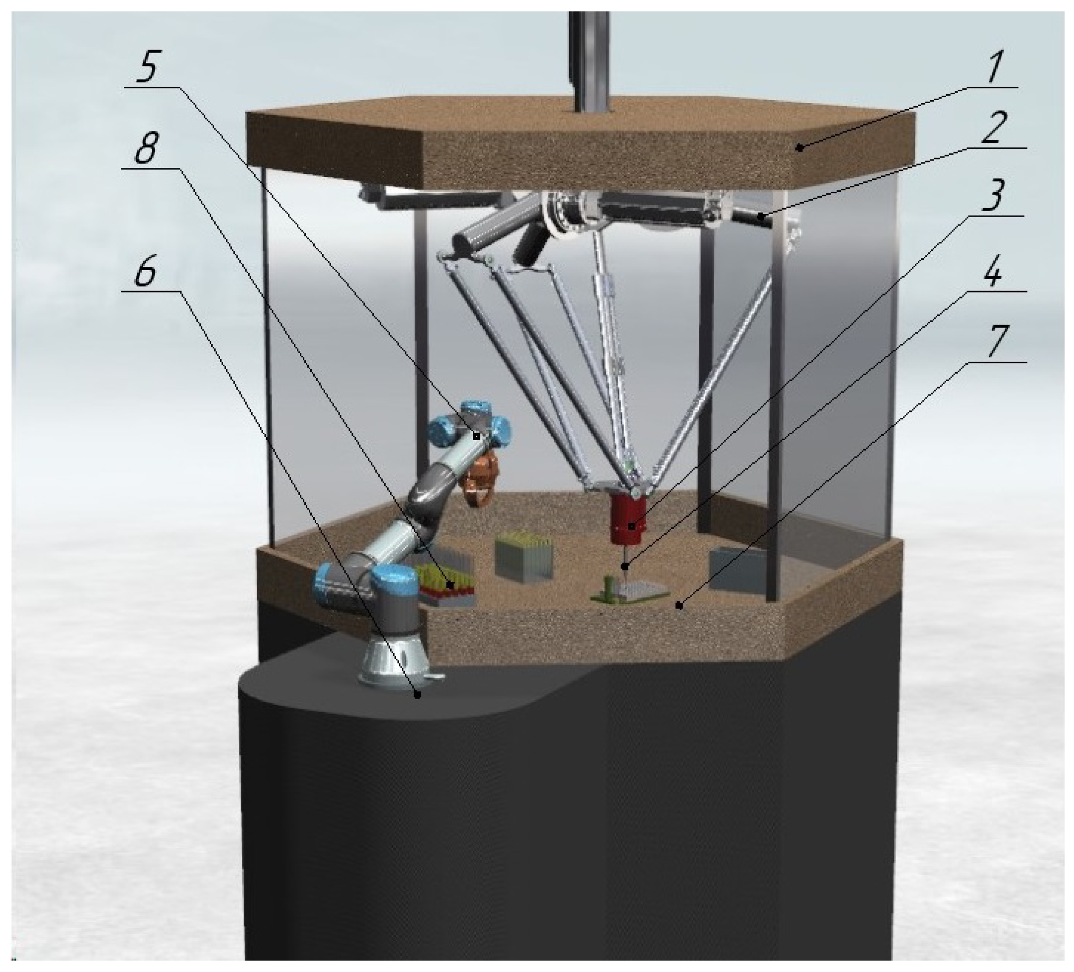
Consider a robotic system [22] consisting of a delta robot equipped with a drip device that performs the aliquoting process, i.e., it dispenses (extracts) the contents of a test tube into separate portions (aliquots), and a serial robot that handles tubes containing biomaterial (Figure 1). The figure illustrates the following components: (1) the body, or non-movable base, of the delta robot; (2) the delta robot itself; (3) the dosing head; (4) the replaceable cap; (5) the serial manipulator; (6) its fixed base; (7) the workspace; (8) a rack holding test tubes.
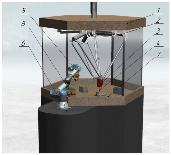
Figure 1.
Robotic aliquoting system.
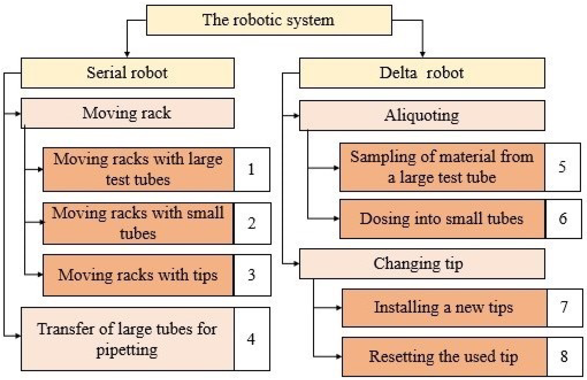
The operations performed during the aliquoting process are shown in Figure 2.
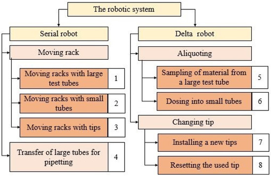
Figure 2.
Operations performed by each of the robots.
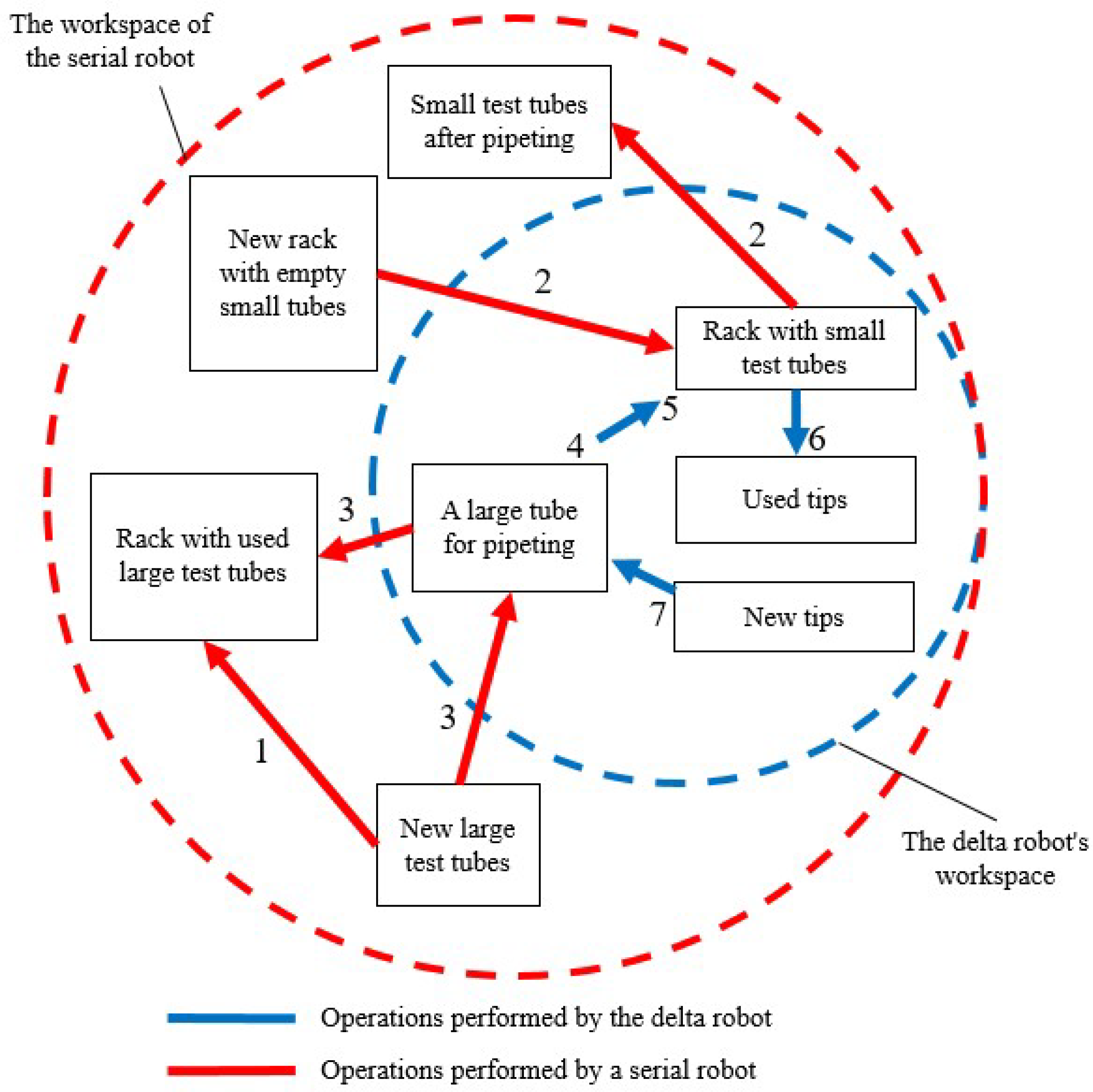
Figure 3 illustrates the aliquoting area, taking into account the operations performed. Each operation is indicated by an arrow with a number, as shown in Figure 2. The blue color represents the workspace of the delta robot and the operations it performs, while the red color represents the workspace and operations of the serial robot. The placement of objects within the area is determined based on the workspace of the delta robot, ensuring that only the objects with which it interacts are positioned within its reach.
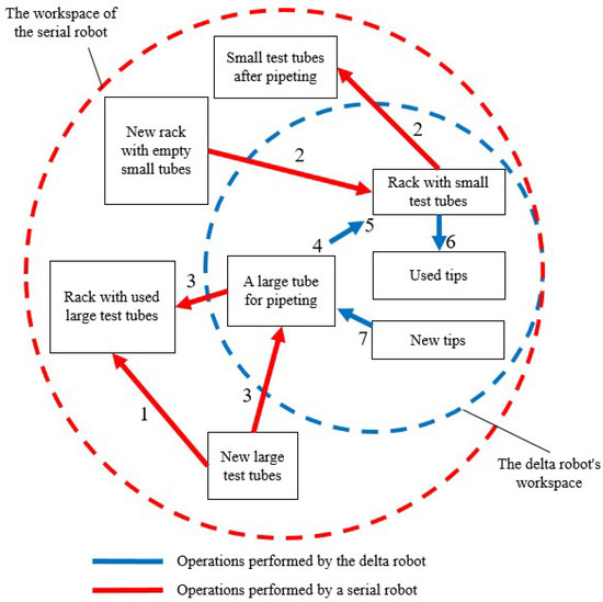
Figure 3.
Aliquoting work safety zone, taking into account the operations performed.(numbers according to Figure 2).
The considered system design and operations determine the features that should be taken into account when choosing the relative position and organizing joint work, in particular the following:
- The workspaces of the robots should intersect, since the robots should perform operations with the same objects (test tubes);
- During operations that do not involve interaction, the areas in which the robot links move should not intersect. This should be taken into account when searching for acceptable ranges of robot movement.
Let us take a closer look at the model of each of the robots included in the system.
2.1. Delta Robot
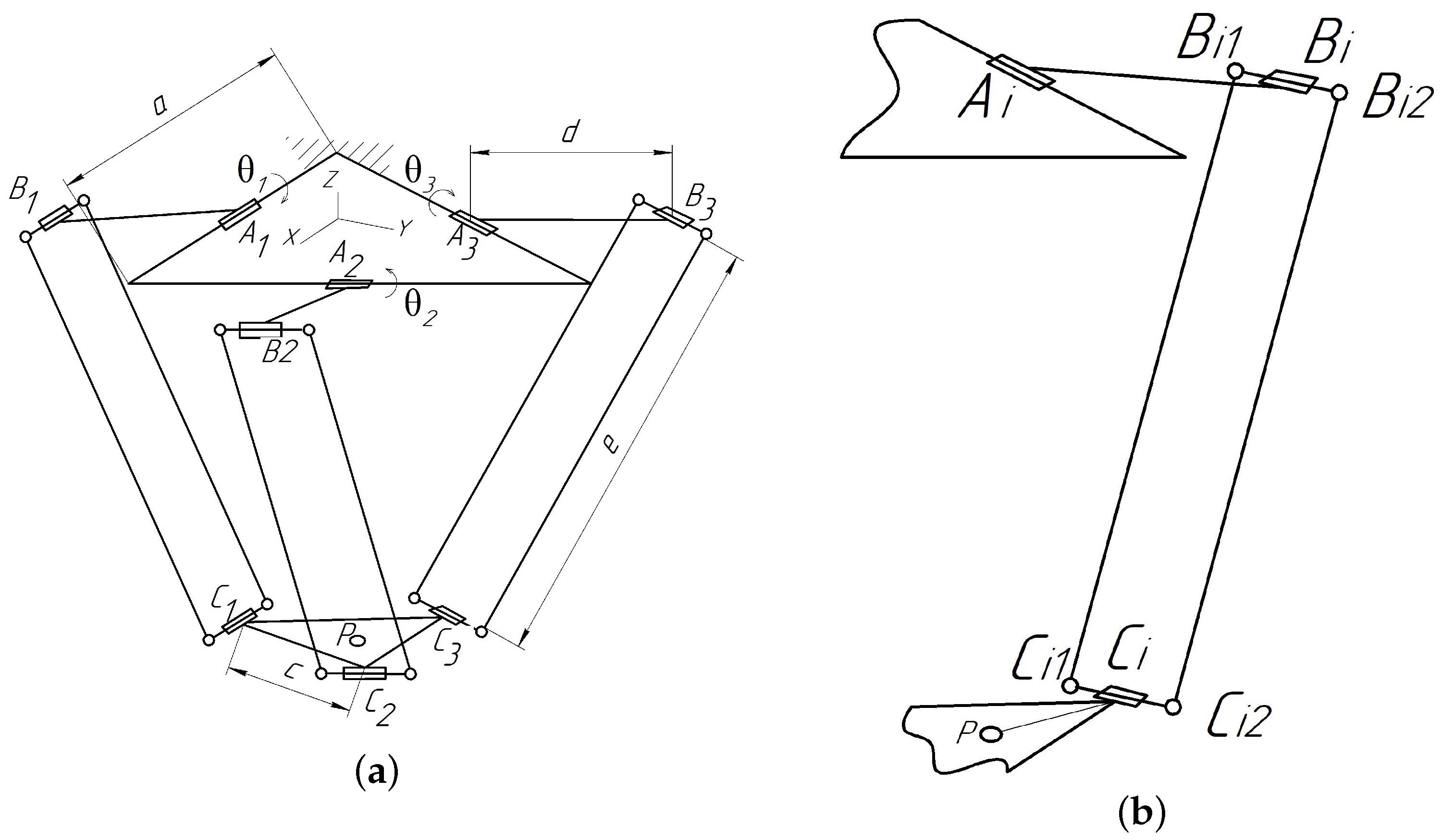
The delta robot is based on a parallel structure mechanism [23], which comprises three parallel kinematic chains suspended from the fixed base at points corresponding to the midpoints of the sides of an equilateral triangle. At their other ends, these kinematic chains are attached to a movable platform at points corresponding to the vertices of another equilateral triangle. Each chain consists of a rod and a joint parallelogram connected to each other. All connections within the mechanism are realized using revolute joints. To change the position of the mobile platform, electric drives are employed, mounted at the attachment points of the mechanism to the base, and are used to adjust the states of the corresponding joints. The delta robot GSK C4-1100 (GSK CNC Equipment Co., Ltd., Guangzhou, China) is used in the work. The kinematic diagram of the delta robot [22] is presented in Figure 4.
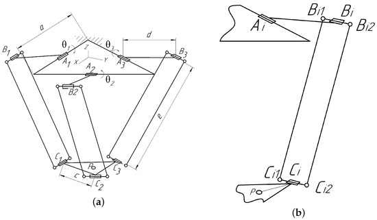
Figure 4.
Kinematic scheme of the delta robot: (a) general scheme; (b) kinematic chain .
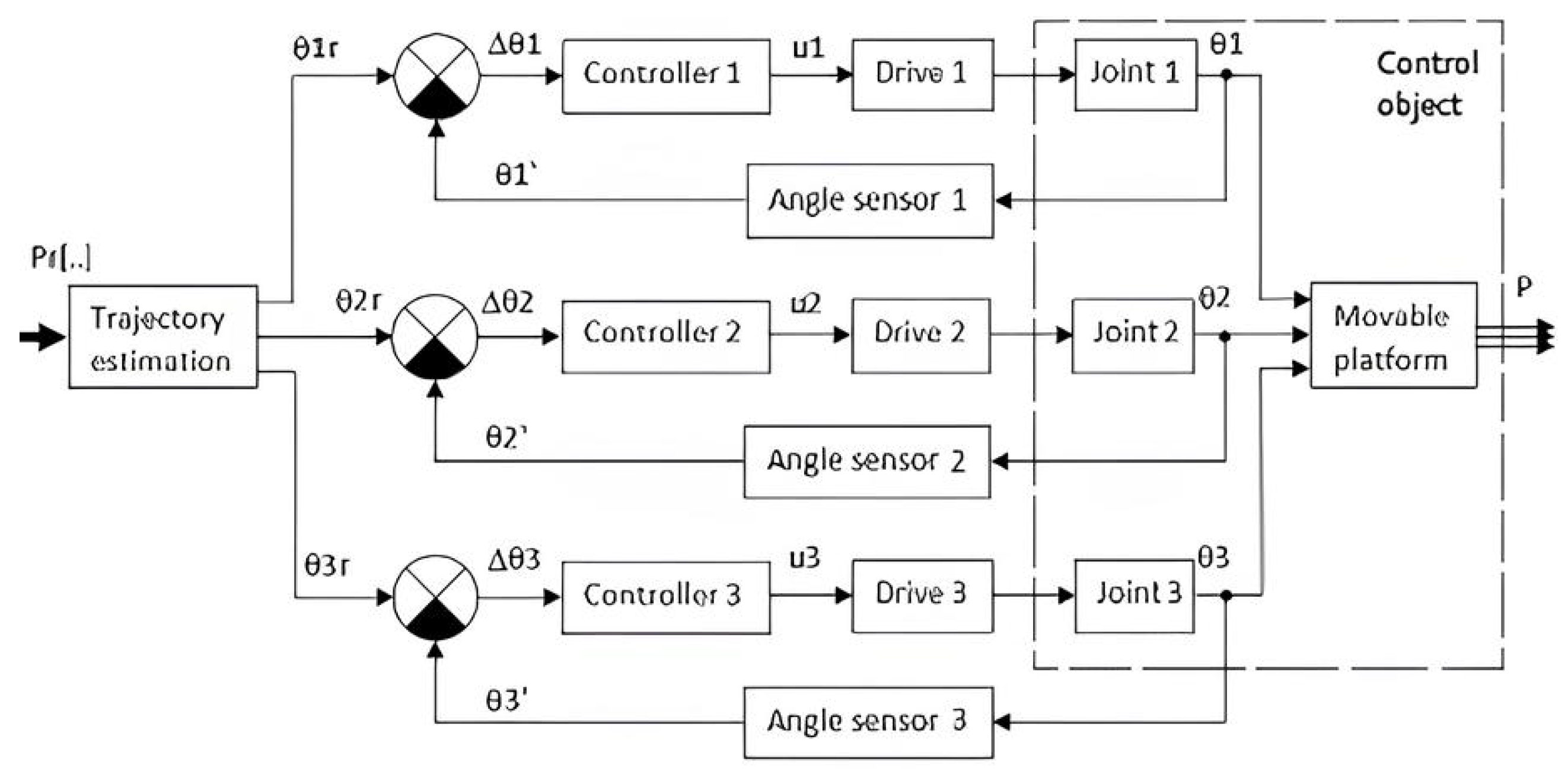
The control of the robot involves adjusting the values of the angles , , and in accordance with the specified trajectory of the x, y, and z coordinates of the center of the mobile platform. The functional diagram of the control system includes a module for calculating the input coordinates of the mechanism, three identical rotation angle control loops, and the mobile platform, whose position is determined by the actual values of , , and . Each of the nested control loops consists of a rotary joint, an electric drive, a controller, and a rotation angle sensor. The desired values of the input coordinates are calculated from the output coordinates by solving the inverse kinematic using the following formula:
where , , and are auxiliary variables that are defined as
where a, c, d, e are geometric parameters of the delta robot described above, and are determined in accordance with Figure 4.
Of the two possible signs in Equation (1), the “” sign corresponds to the “correct” orientation of the mechanism links.
Let us write down the formulas for determining the coordinates of the joint centers of the delta robot (see Figure 4), which are necessary for determining the position of the links.
2.2. Serial Robot
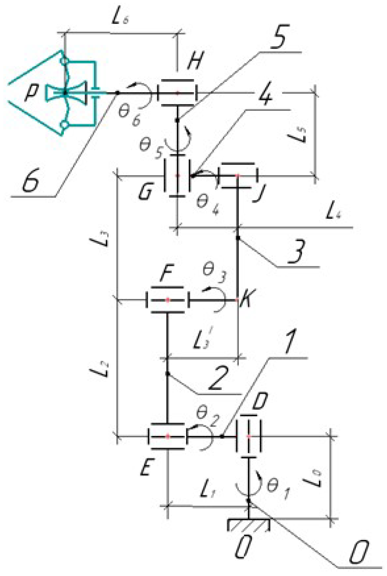
Let us consider a mathematical model of a serial robot. Figure 5 presents a block diagram of a serial robot. The lengths of the links are denoted as , where . The joint rotation angles are denoted as , where .

Figure 5.
Block diagram of a serial robot (0–6: robot links).
Let us write down the formulas for determining the coordinates of the joint centers (D, E, F, G, H) and the points K and J located on the link FG, which are required to determine the positions of the links. In this case, we denote as and as .
where
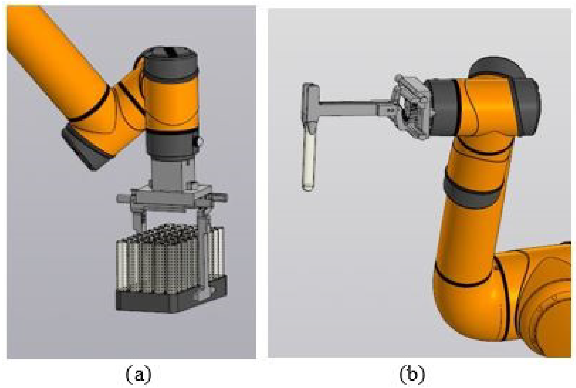
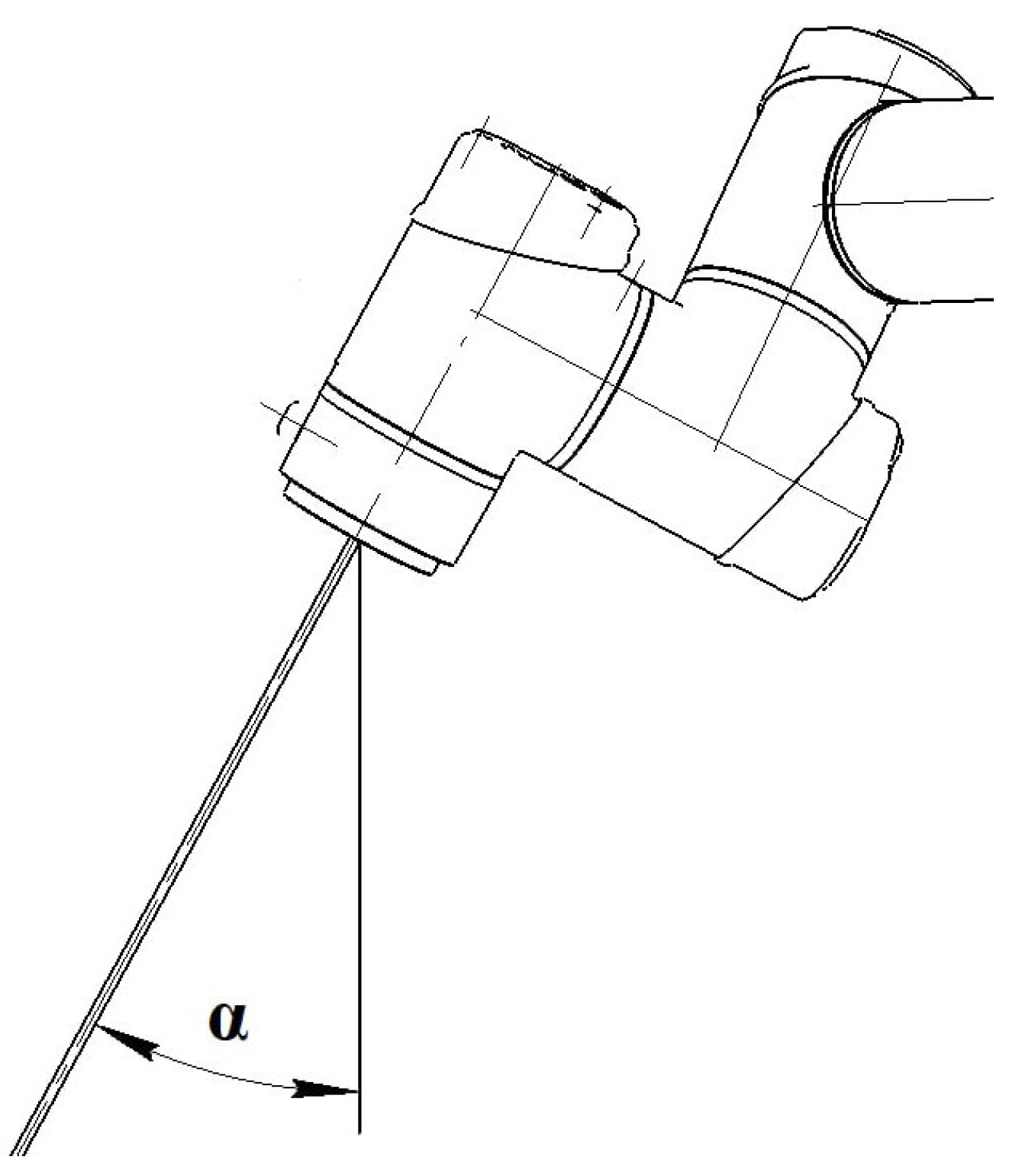
During the aliquoting process, there are constraints on the orientation of the end effector of the serial robot, which take into account the specific features of the gripping device used [24]. When the robot performs the operation of transferring a rack, the orientation of the normal plane of the flange of the end effector should remain close to vertical (Figure 6a). To achieve this, we introduce a constraint on the angle between the normal and the vertical axis (Figure 7).
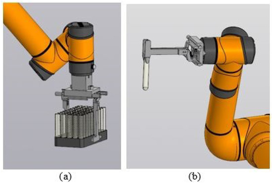
Figure 6.
Operations performed by a serial robot: (a) moving a rack; (b) moving a test tube.

Figure 7.
Limitation on the orientation of the end effector during work safety zone.
During the tube transfer operation, the orientation of the normal plane of the flange of the end effector should remain close to horizontal (Figure 6b). In this case, the constraint on the angle takes the following form:
Summarizing the mathematical model obtained in this section, the following can be highlighted:
- Formula (1) is a solution to the inverse kinematics for a delta robot and is necessary both for calculating the coordinates of the links in subsequent formulas and for checking the reachability of the position, which will be used in subsequent sections.
3. Algorithm for Determining the Work Safety Zone
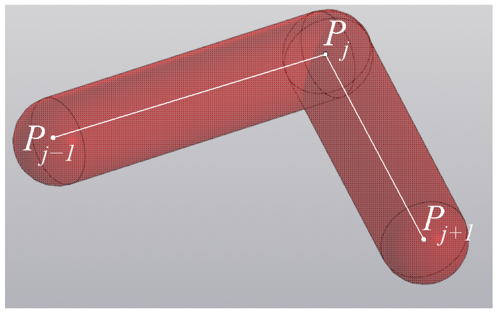
A huge amount of work is devoted to defining the workspace (the set of possible positions and orientations of the robot end effector). At the same time, no attention is paid to defining the entire space that the robot links need for safe operation. In previous studies, we proposed an algorithm for defining such a space [25]. However, it used assumptions on the radii of the links that were not taken into account, resulting in a space that was smaller than its actual dimensions. In the case of small radius values, the error is insignificant, but with an increase in the radii, it increases. In the current study, the methodology has been modernized, taking into account the radii of the links. The algorithm is universal and applicable to robots of various structures. In the context of the current work, determining the zones that robots need to perform operations is important for determining the permissible ranges of motion of a serial robot in order to eliminate collisions between a delta robot and a serial robot. The work safety zone will be understood as an area of three-dimensional space within which all robot links can be located for a given range of robot positions. Let us imagine the robot links as spherocylinders (cylinders with two hemispheres at the ends). In most cases, the centers of the hemispheres coincide with the centers of the robot joints (point in Figure 8), but in some cases they can be specified at other points, taking into account the maximization of the correspondence of the decomposed model to the real robot design. An example of such a case is point K at the bending point of the serial robot link in Figure 5. For a more convenient designation of all points that are the centers of the hemispheres of the spherocylinders, we call them anchor points.
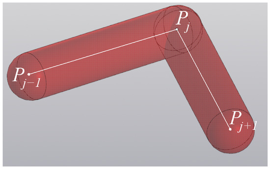
Figure 8.
Representation of robot links.
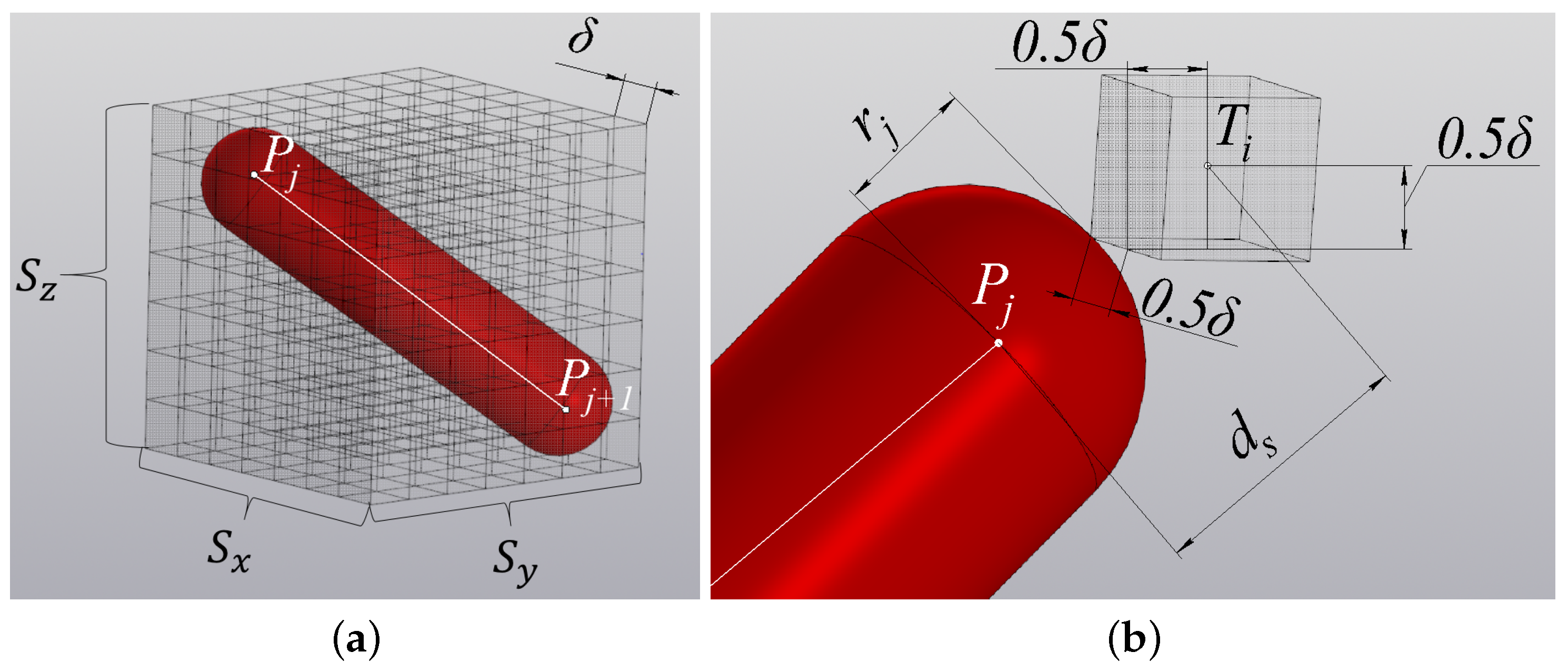
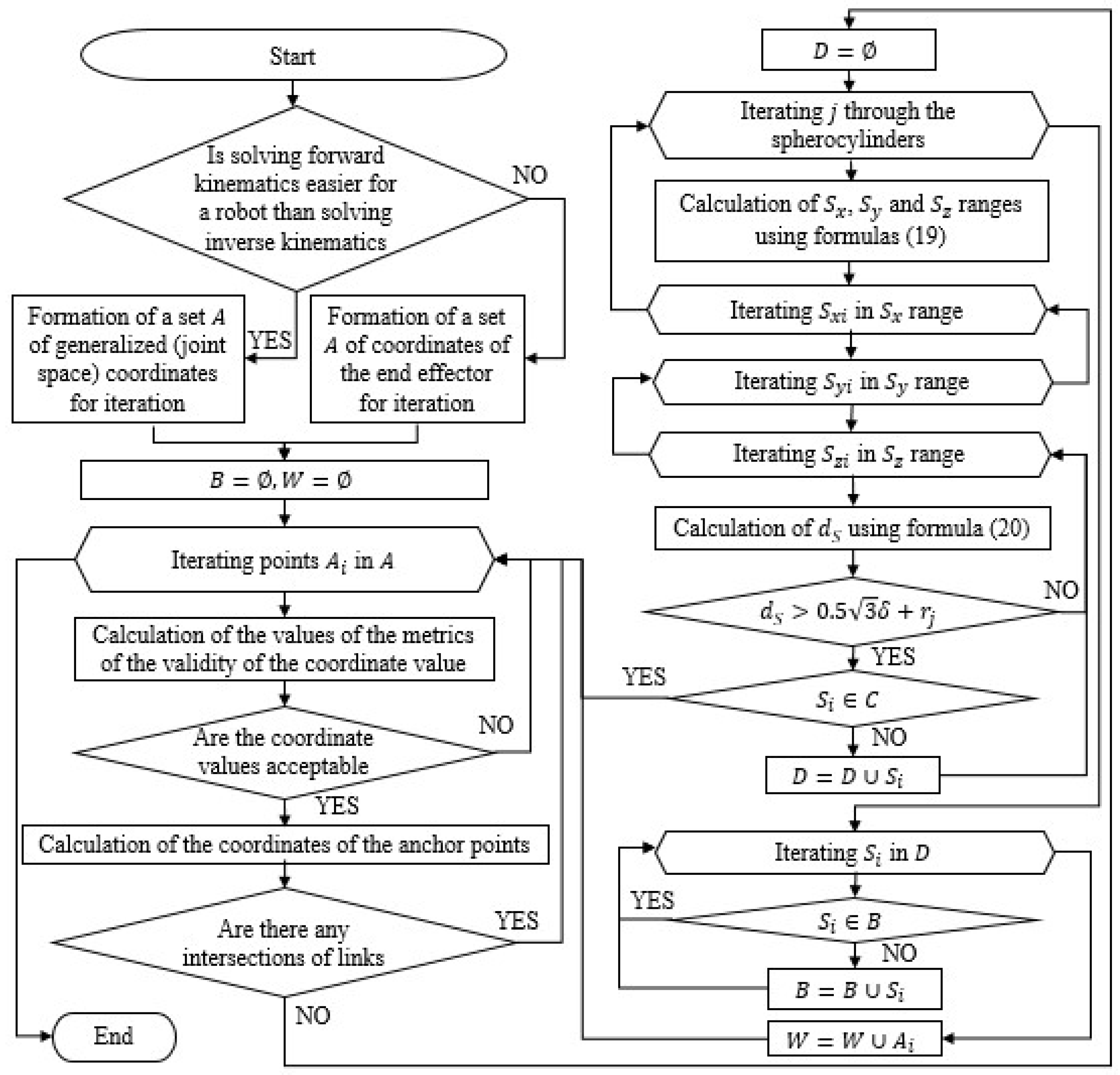
Let us consider the algorithm for determining the work safety zone (Figure 9). At the beginning of the algorithm, a set of points is formed in the generalized (joint space) coordinates’ space or in the coordinates of the end effector space, depending on which is easier to obtain, a solution to the forward kinematics or a solution to the inverse kinematics. For example, for a delta robot, as for most parallel robots, it is easier to obtain a solution to the inverse kinematics (1). Therefore, it is more convenient for the delta to form a set A in the coordinates of the end effector space, since it is easy to check their reachability for these coordinates and calculate the anchor point coordinates. Whereas it is easier for a serial robot to obtain a solution to the forward kinematics (Equation (15)). Therefore, it is more convenient for him to form a set A in the generalized (joint space) coordinate space. Next, an empty set B of points of the safety zone and an empty set of workspace W are created. Creating a workspace set is not necessary for defining a safety zone, but if it is needed to define both sets; this allows us to avoid performing the same check for points from A again. After that, the search begins for all the points in set A. For each of them, metrics of relevance of the values of this point are calculated. For example, for a delta robot, such metrics are position reachability and the absence of singularities. In the course of the current study, the condition for the positivity of root expression in (1) was used to verify reachability. To verify singularities, the condition for sign invariance of the determinant of the Jacobi matrix [22] was used. If the position in question is acceptable, the anchor point coordinates are calculated. For a delta robot, these are Formulas (2)–(9), for a serial robot, they are Formulas (10)–(15). Then, a check is performed on the intersections of the links. In the current work, the approach described earlier by the authors in [26] is used to check the intersections. If there are no intersections, is added to the workspace W (this operation can be skipped if the workspace definition is not required). Then, the enumeration of spherocylinders begins. The centers of the hemispheres of the spherical cylinders are located in anchor points, and the radius of the cylinder corresponds to the radius of the link to which it corresponds. To limit the number of points forming the work safety zone, a discretized space is used, taking into account the accuracy of the approximation . That is, each of the points in the space , corresponds to a certain point (cell of the discretized space) , , which is calculated as
where is the accuracy of the approximation, and [ ] is the rounding operation here and further in this section. Taking into account the discretized space, there are ranges , , and for each of the spherocylinders, which completely include the spherocylinder (Figure 10a). Define the upper and lower boundaries of the range as
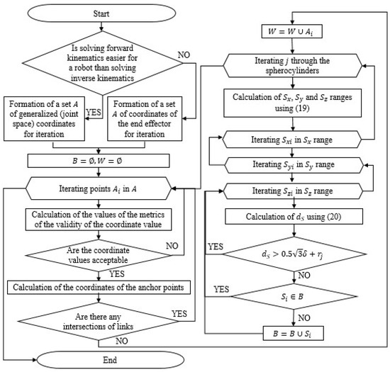
Figure 9.
The algorithm for determining the work safety zone.
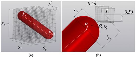
Figure 10.
Cells of the discretized space: (a) ranges for one spherical cylinder; (b) the maximum distance from the center of the cell to the anchor point of the spherical cylinder, if there is an intersect.
The boundaries of the and ranges are defined similarly. After calculating the ranges , , , the algorithm iterates through all possible values within the calculated ranges. For each of the points , the distance from the center of the cell to the segment is calculated
where = (,,), t is the projection parameter that shows at which point of the segment is the closest point to the point and is calculated as
Let us write down the condition of a guaranteed absence of intersections between the spherical cylinder and the cell .
This is obtained based on an estimate of the maximum possible distance at which an intersection can occur (when the spherical cylinder touches the top of the cell), as shown in Figure 10b. If the condition (22) is not satisfied, then a check is performed for the point to enter the array B of the work safety zone. If is not included in array B, then is added to B. After iterating through all points in the range , , , the transition to the next spherical cylinder is performed. After the iteration of all the spherical cylinders is completed, the transition is performed to the next point in the array A. After the end of the iteration of points in A, the algorithm completes its work. The result is an array of work safety zone B.
The above algorithm can be used for various structures of individual robots without taking into account other robots working nearby. In the case of several robots, as, for example, in the considered system for aliquoting, this algorithm can be used to determine the work safety zone of one robot (for example, delta), but to determine the work safety zone of the second robot (for example, serial), an algorithm supplemented with a check for the absence of intersections of work safety zones at the moment of its formation can be used. Let us consider the supplemented algorithm in more detail (Figure 11). Unlike the previous algorithm, this one uses several additional sets. First, there is the set C of the work safety zone of another robot. It is used to check each of the points belonging to the set C. If at least one of the points belongs to C, this means that one of the robot links in this position can collide with another robot. Therefore, during the algorithm, the point is added to the array W not before the enumeration of the spherocylinders but only after checking all the points for this position to ensure that they are not included in C. Similarly, the points are not immediately entered into B but are first entered into the auxiliary set D, and only after a successful check of all the spherocylinders of the current position are those points from D that do not yet belong to B entered into it.

Figure 11.
The algorithm for determining the work safety zone, taking into account the work safety zone of another robot.
We use synthesized algorithms to determine the location and permissible ranges of motion of a serial robot, taking into account the workspace and work safety zone of a delta robot.
4. Determination of the Location and Permissible Ranges of Motion of the Serial Robot
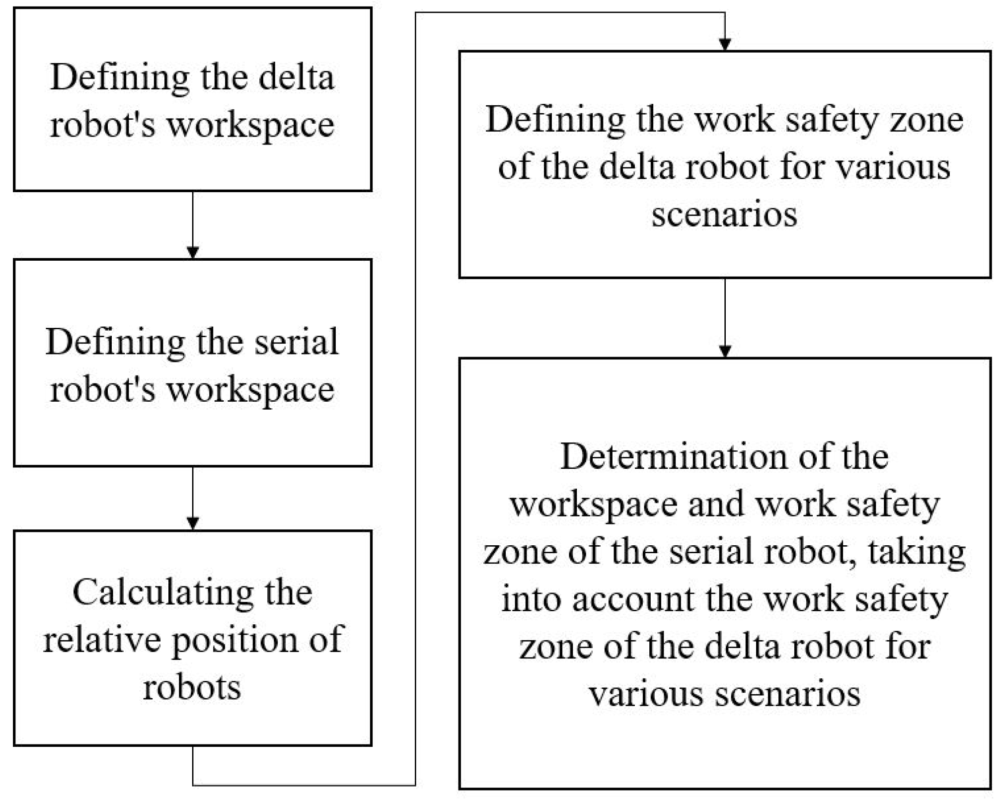
The proposed approach to determine the relative position of robots in the system as well as the permissible ranges of motion of a serial robot, taking into account the exclusion of collisions in various scenarios, includes the steps shown in Figure 12.
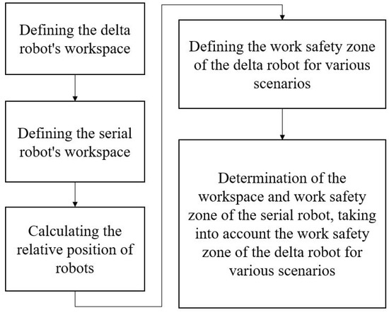
Figure 12.
The stages of determining the relative position and permissible ranges of motion.
Let us consider each stage in detail.
4.1. Defining the Workspace of the Delta Robot
The constraints of the workspace take into account the reachability of positions and the absence of failures in the robot’s operation. Reachability assumes the existence of such drive angles , at which the lengths of the kinematic chains will be sufficient for the robot to be in this position. This can be taken into account by limiting the value of the radical expression in Equation (1). The absence of failures in the robot’s operation assumes the exclusion of loss of control (singularity), which can be taken into account by the constancy of the Jacobian matrix. Collisions of links with each other can also be attributed to failures in operation. The algorithm for exclusively determining the working space, taking into account all these constraints, is described in [13].
4.2. Defining the Workspace of the Serial Robot
The definition of the workspace is performed using the algorithm in Figure 11, but without enumeration of the spherical cylinders and the formation of the work safety zone. Thus, it consists of a sequential discrete enumeration of the input coordinates with a given step size, followed by calculating the coordinate values of the centers of the joints and reference points of the links for each node using Formulas (10)–(15). For each position, if the workspace permits moving a rack, condition (16) is verified, while conditions (17) are applied for moving test tubes. Subsequently, link intersections are checked using a geometric approach based on calculating the minimum distance between segments connecting the joint centers, as described in detail in [26]. If no intersections are detected, the coordinates of the end effector are added to the workspace array. At this stage, the coordinates of the base O of the serial robot in the coordinate system of the delta robot are unknown and are assumed to be zero, i.e.,
4.3. Calculating the Relative Position of Robots
We denote the covering set of the workspace of the delta robot as and the covering set of the workspace of the serial robot as . In accordance with the proposed concept of the relative arrangement of workspaces, illustrated in Figure 3, it is proposed to align the extreme achievable positions of the robot workspaces on one side. With this in mind, the coordinate of the base of the serial robot in the coordinate system of the delta robot is calculated as follows:
The coordinate is assumed to be zero due to the symmetry of the workspaces relative to the x-axis.
The coordinate is calculated based on the attachment of the serial robot to a desktop having a height at which the horizontal end of the delta robot has a maximum diameter, that is
4.4. Defining Work Safety Zone of the Delta Robot for Various Scenarios
We use the algorithm for determining the work safety zone without taking into account the second robot (Figure 9). Let us consider the scenarios for performing delta robot operations that affect the formation of the array A of the end effector positions at the beginning of the algorithm. Anchor points in each of the scenarios are calculated using Formulas (2)–(9). Let us denote the work safety zone of the delta robot as .
Scenario 1. The delta robot is positioned at its home position , the coordinates of which are calculated as follows:
where .
Therefore, the initial array A in the algorithm for determining the work safety zone will consist of one point .
When the delta robot is in the home position, the serial robot performs operation 2 according to Figure 2 and Figure 3.
Scenario 2. The delta robot performs the aliquoting process (operations 6 and 7, according to Figure 2 and Figure 3). To allow the serial robot to perform operations 3–4 simultaneously, we introduce a constraint on the position of the delta robot. The workspace of the delta robot for this scenario is denoted as .
Thus, the array in the algorithm in Figure 9. The condition is the metric of the admissibility of the position, since the delta robot performs dosing in the right part of the system.
Scenario 3. In addition to the two scenarios mentioned above, there is a third scenario where the serial robot performs operation 4 while the delta robot performs operation 5. This scenario involves potential robot interaction. In this case, the work safety zones of the robots may overlap, necessitating the consideration of interaction options during the scenario. This will be discussed in detail in Section 5.
4.5. Defining the Workspace and Work Safety Zone of a Serial Robot, Taking into Account the Work Safety Zone of a Delta Robot Under Various Scenarios
Let us consider the problem of defining the work safety zone of a serial robot for the first two scenarios. For this, the algorithm shown in Figure 11 is used. The set A contains joint coordinates . The anchor points are calculated using Formulas (10)–(15). The metrics of position admissibility are the condition for the admissibility of the angle (according to condition (16) for transferring racks and according to condition (17) for transferring test tubes). In the case of determining the workspace without taking into account the orientation of the end effector (for free movement), the condition for the admissibility of the angle is not satisfied. The set C in the algorithm is equal to the work safety zone of the delta robot of the scenario under consideration.
Let us consider the application of the synthesized algorithms for selecting the relative position of the robots and determining the workspace and work safety zones for various scenarios.
5. Results of Modeling of Workspaces and Work Safety Zones
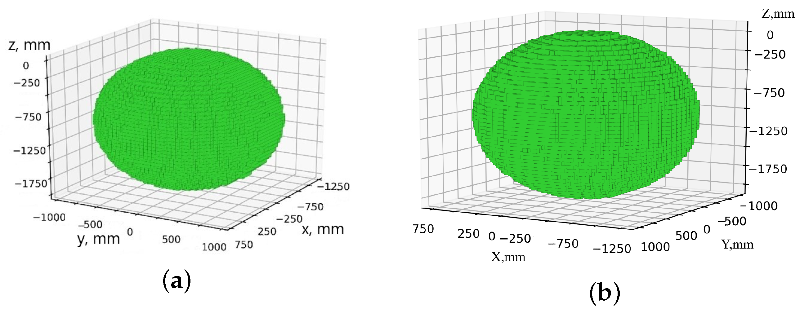
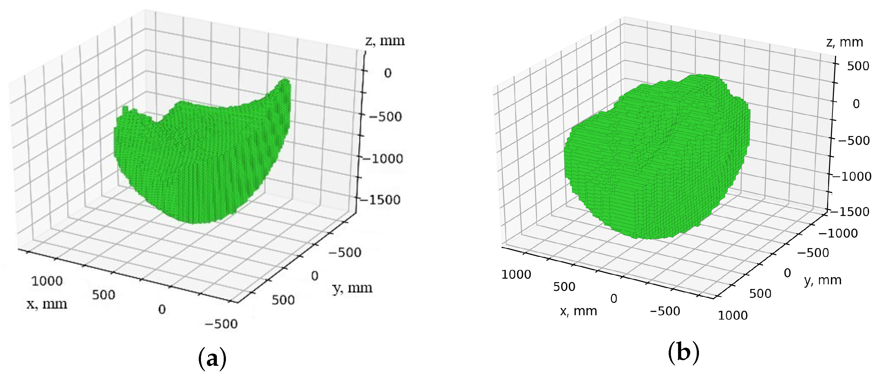
The algorithms are implemented programmatically in the C++ programming language using the OpenMP library for parallel computing. The simulation results are exported as JSON files and are subsequently utilized for visualization through custom Python (3.8.10) scripts leveraging the Matplotlib (3.1.2) library. The simulation was performed for the following geometric dimensions of the delta robot: mm, mm, mm, and mm; the dimensions of the serial robot: mm, mm, mm, mm, mm, mm, mm, and mm; permissible deviation of the orientation of the end effector of the serial robot ; approximation accuracy mm. Figure 13 presents the results of modeling the workspace and work safety zone for a serial robot. As can be observed from the figure, the shape and size of these areas exhibit minimal differences, primarily because the boundary positions of both the work safety zone and the workspace are largely determined by the position of the end effector. Meanwhile, the remaining links are positioned closer to the robot attachment point, resulting in negligible deviations between the two zones.

Figure 13.
Areas of the serial robot: (a) workspace; (b) work safety zone.
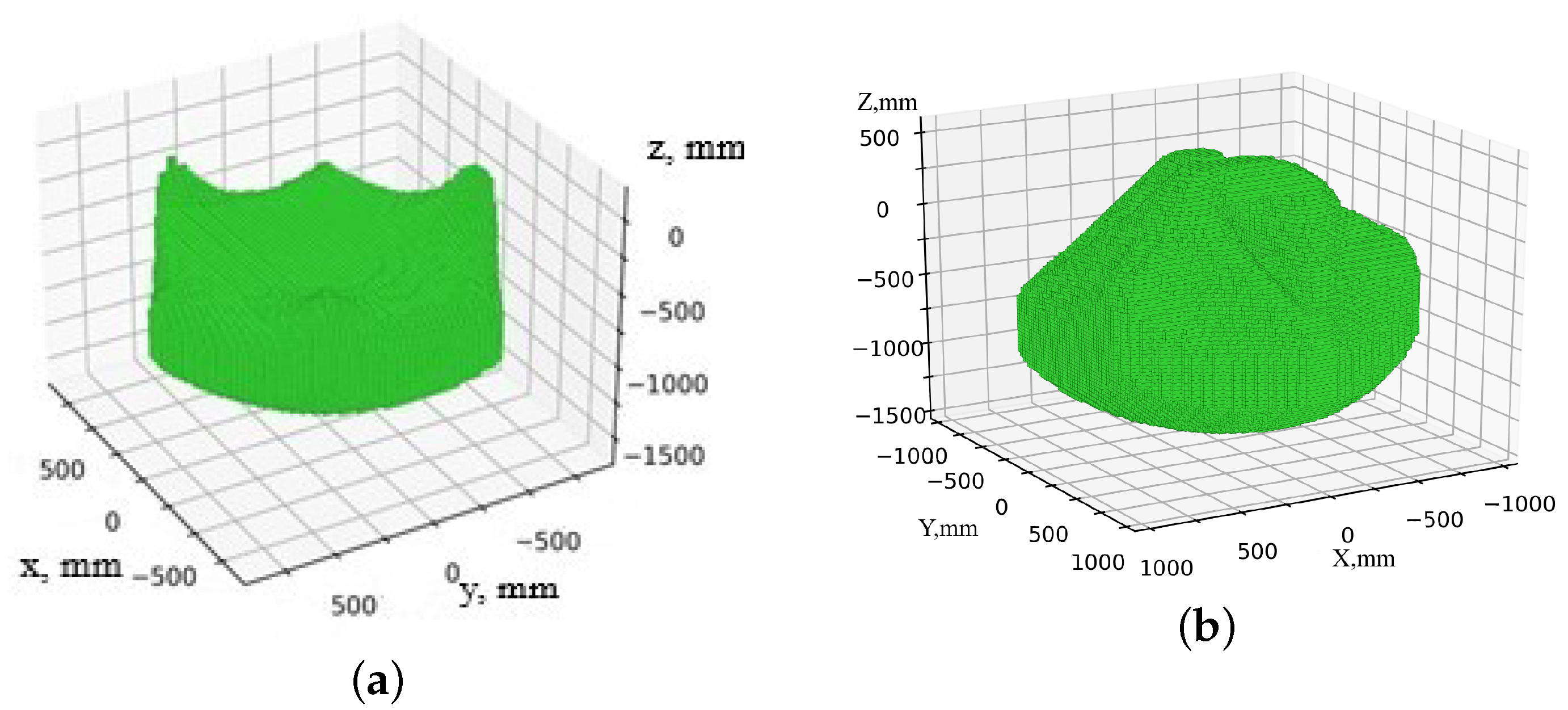
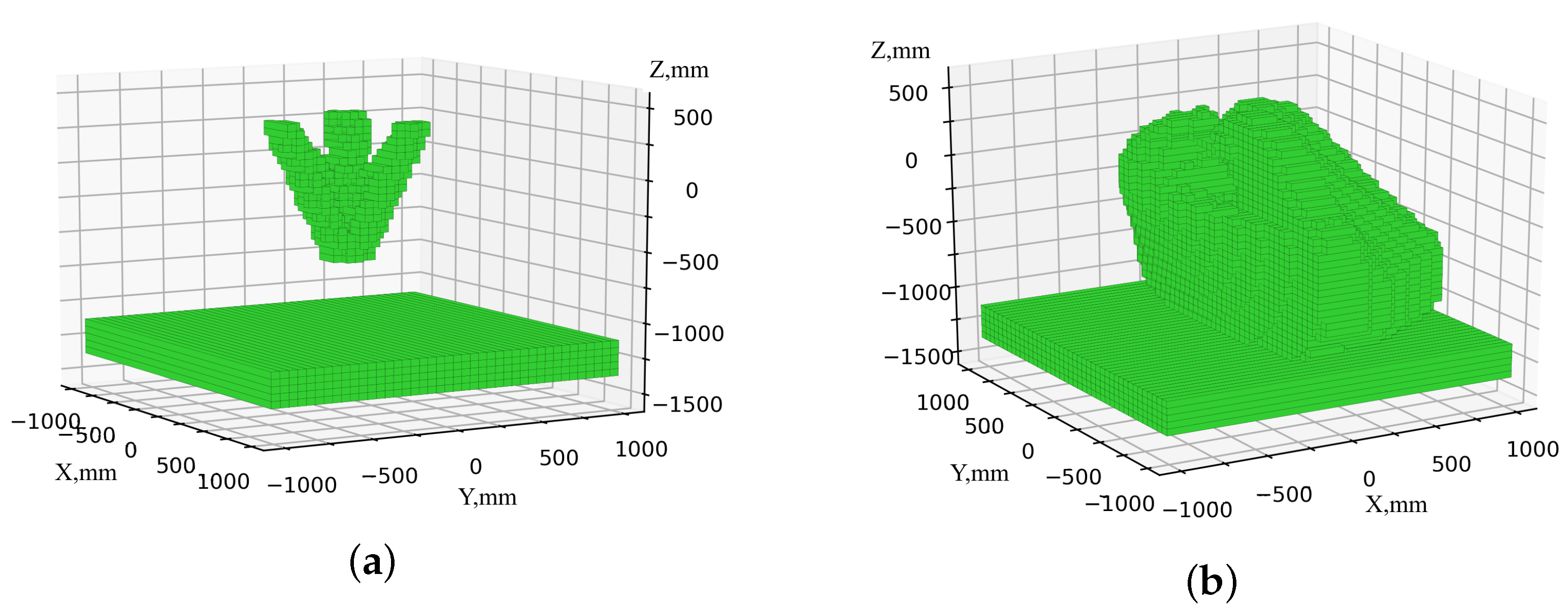
Figure 14 shows the results of modeling the workspace and work safety zone of a delta robot. In this case, the shape and dimensions are different, since the upper part of the work safety zone is formed due to the movement of intermediate links.

Figure 14.
Areas of the delta robot: (a) workspace; (b) work safety zone.
Based on the obtained workspaces and the methodology for determining the relative position of the robots proposed in Section 4.3 the following position of the attachment point of the serial robot was selected:
As a result of the workspace analysis, the home position of the delta robot was selected.
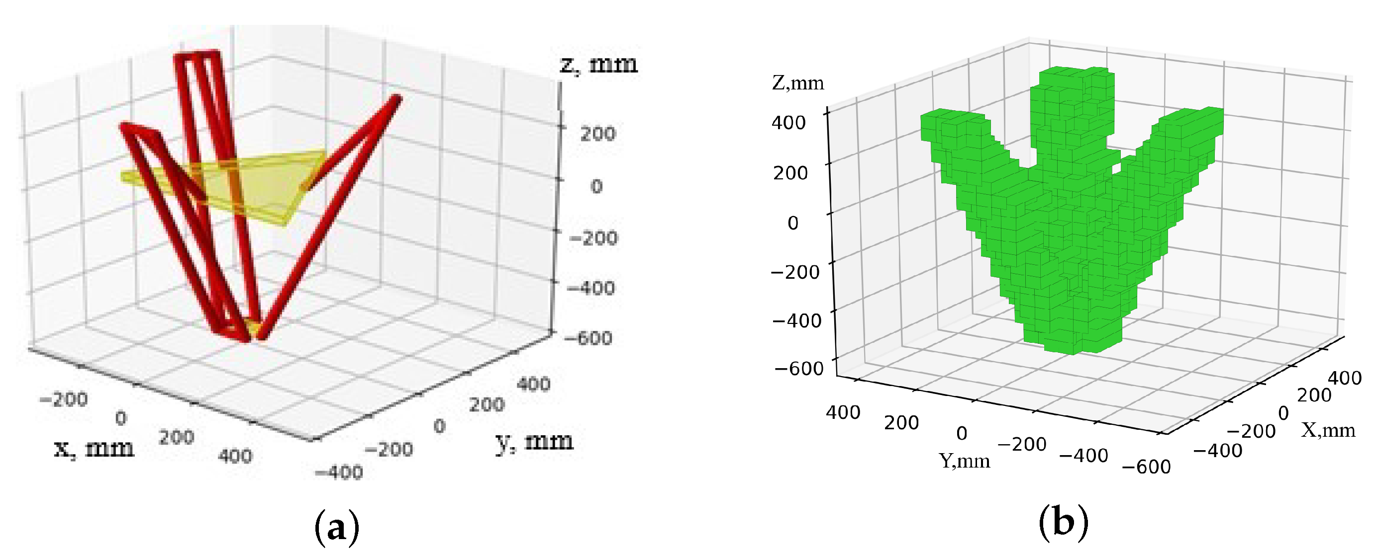
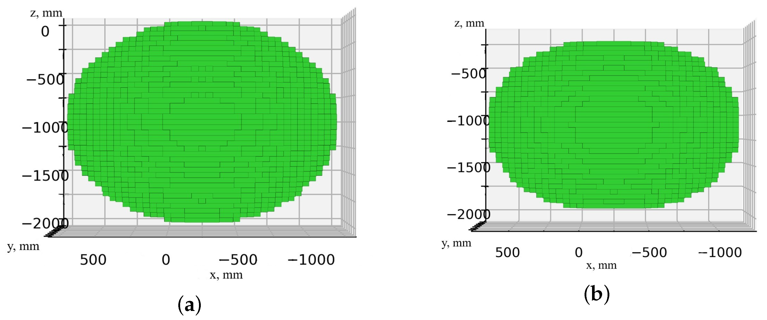
To determine the permissible operating sequences for the different scenarios, the work safety zones of the delta robot were constructed for the two scenarios discussed in Section 4.4 The results are presented in Figure 15b (scenario 1) and Figure 16b (scenario 2). As can be observed from the comparison of Figure 16a,b, the dimensions of the workspace and the work safety zone also differ.
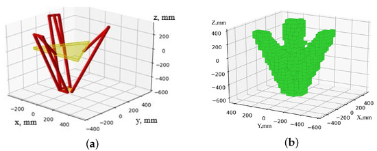
Figure 15.
Home position of the delta robot: (a) visualization of the position; (b) work safety zone.
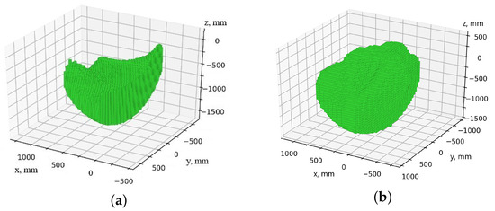
Figure 16.
Areas of the delta robot during dosing: (a) workspace; (b) work safety zone.
Since the work safety zone of the delta robot, as well as the permissible workspace of the serial robot, is also affected by the presence of a table, a set of points corresponding to the table’s surface is added to the work safety zone of the delta robot (Figure 17).

Figure 17.
Areas that are unacceptable for a serial robot: (a) when the delta robot is in the home position; (b) during dosing.
Taking into account the obtained work safety zone, the simulation of the workspace and work safety zone of the serial robot was performed. Based on the simulation results, a comparison of workspaces was conducted, considering both the inclusion and exclusion of the delta robot work safety zone, as well as the presence or absence of restrictions on the orientation of the end effector. Figure 18 presents the results without accounting for the delta robot work safety zone. As can be observed from the figure, the size of the workspace of the serial robot (Figure 18a) decreases when restrictions on the orientation of the end effector are introduced (Figure 18b).

Figure 18.
Workspace of a serial robot with various restrictions on the orientation of the end effector: (a) without restrictions; (b) with restriction (16) on the angle .
Subsequently, modeling was carried out for scenarios 1 and 2, taking into account the presence of the table and the work safety zones of the delta robot. Table 1 provides a comparison of the workspace volume for each scenario under different constraints on the orientation of the end effector of the serial robot. The simulation results are presented in Figure 19 and Figure 20.

Table 1.
The amount of workspace of a serial robot for various scenarios.
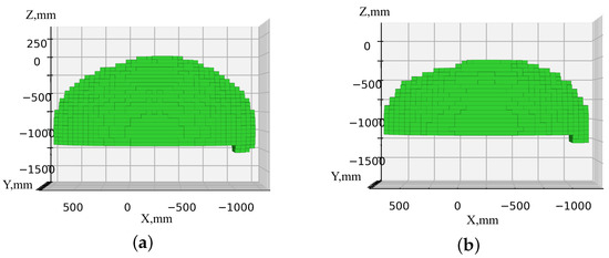
Figure 19.
Permissible workspaces of a serial robot, taking into account the table and the delta robot in the home position, with various restrictions on the orientation of the end effector: (a) without restrictions; (b) with a restriction (16) on the angle .
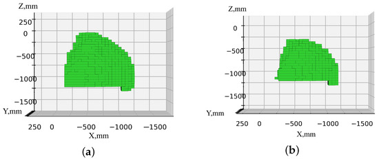
Figure 20.
Permissible workspaces of the serial robot, taking into account the presence of the table and the delta robot during dosing, as determined under various restrictions on the orientation of the end effector: (a) without restrictions; (b) with a restriction (16) on the angle .
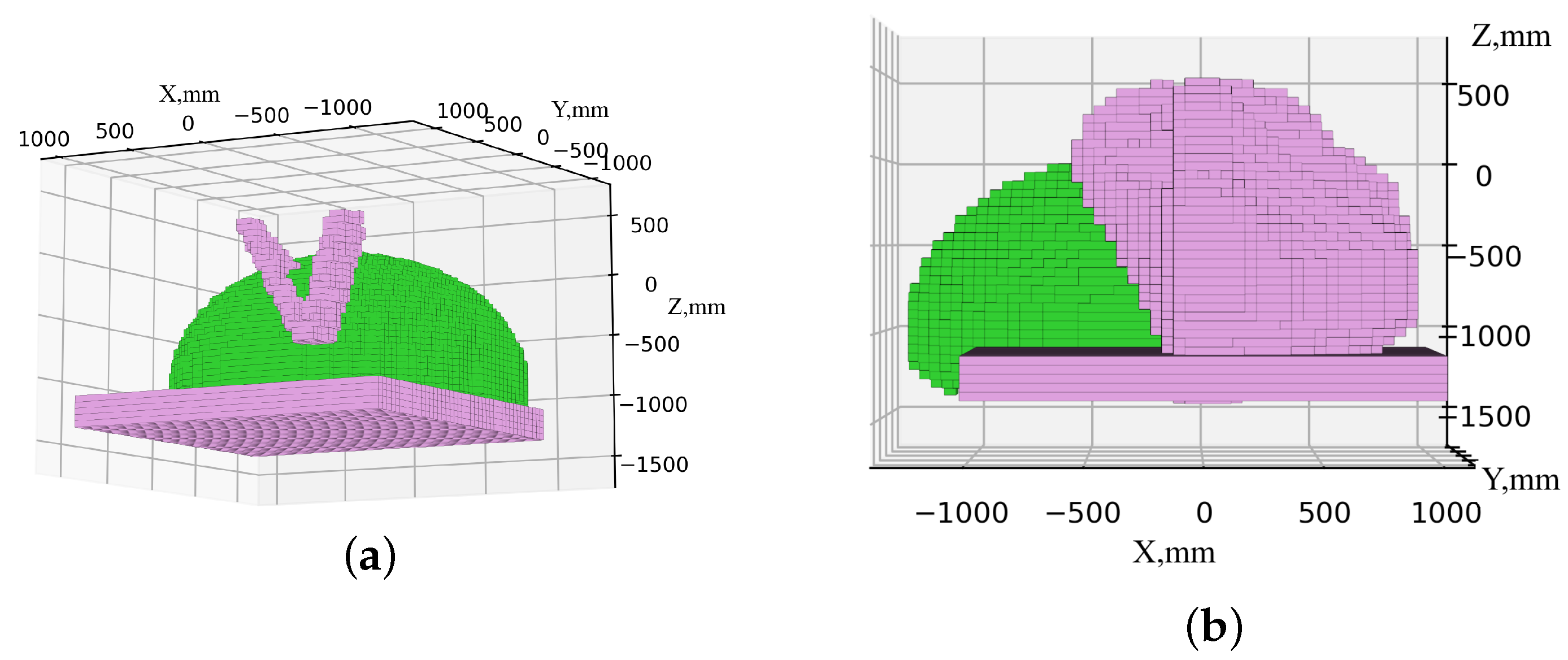
Subsequently, we verified the absence of intersections between the work safety zones by combining the work safety zones of the robots, as illustrated in Figure 21. In the figure, the green color represents the work safety zone of the serial robot, while the purple color corresponds to the delta robot.
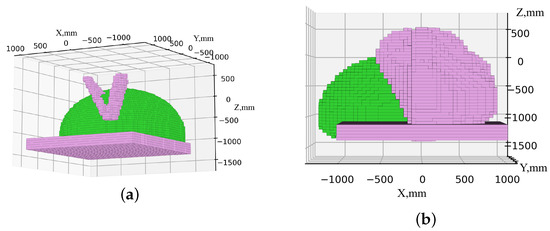
Figure 21.
Combining the work safety zone of robots: (a) scenario 1; (b) scenario 2.
The resulting workspaces are utilized to constrain the movement of the robots during the execution of operations in scenarios 1 and 2 separately. This ensures that there are no collisions between robots during operations that do not require their interaction. Next, we will consider the interaction of robots within the framework of scenario 3 (when performing operations 4 and 5 in accordance with Figure 2 and Figure 3). In this case, ensuring the absence of intersections does not make sense, since the opposite is required—a common area for manipulating test tubes.
6. Analysis of Robot Interaction
During scenario 3, the serial robot must bring a test tube to the delta robot, from which the delta robot must obtain biomaterial for dosing. The interaction between the robots lasts approximately 10–20 s, depending on the volume of the biomaterial to be aspirated. During this period, the serial robot holds the biomaterial tube stationary, while the delta robot lowers the pipette (the replaceable tip of the dosing device) into the tube. Initially, the pipette moves quickly, reaching slightly below the upper liquid level, followed by a slower descent synchronized with the aspiration process. Once the lower liquid level is reached (with some margin), the pipette is retracted from the tube. Upon completion of the interaction, the serial robot places the tube containing the spent biomaterial on a rack, then moves to another rack with new test tubes, picks up one of them, and slowly moves it to the photographing area to minimize significant vibrations on the liquid surface. In the photographing area, the robot rotates the test tube to identify the optimal angle for determining the required levels and boundaries of the fractions. Subsequently, the tube is moved to the interaction point for aspiration. Since the movement of a tube containing liquid must occur at a slower speed compared to that of an empty tube, in order to enhance the efficiency of the robotic system, it is preferable, all other factors being equal, to organize the robot interaction directly at the photographing point. Following the completion of the interaction, the delta robot moves the dosing device to the aliquot site, where it dispenses the collected liquid in a controlled and precise manner. Subsequently, the receiver of the pipetting device is replaced, and the robot returns to the interaction point. During the aliquoting process, the accurate positioning of the pipetting device is essential; therefore, the robot moves it slowly. As a result, the volume of the aliquoted biomaterial substantially influences the duration of the delta robot’s preparation for the next interaction. In the case of a large liquid volume, the delta robot may return to the interaction point immediately, causing the serial robot to wait, which results in a time loss. In such situations, it is advisable to consider relocating the interaction point along the trajectory of the serial robot closer to the rack containing the spent biomaterial. In the course of the study, a delta robot was simulated in the MATLAB R2021a environment (Figure 22 and Figure 23). In this case, the general scheme was used for mechanisms with three parallel kinematic circuits (Figure 4).
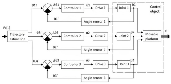
Figure 22.
Functional diagram of the control system.
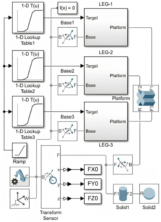
Figure 23.
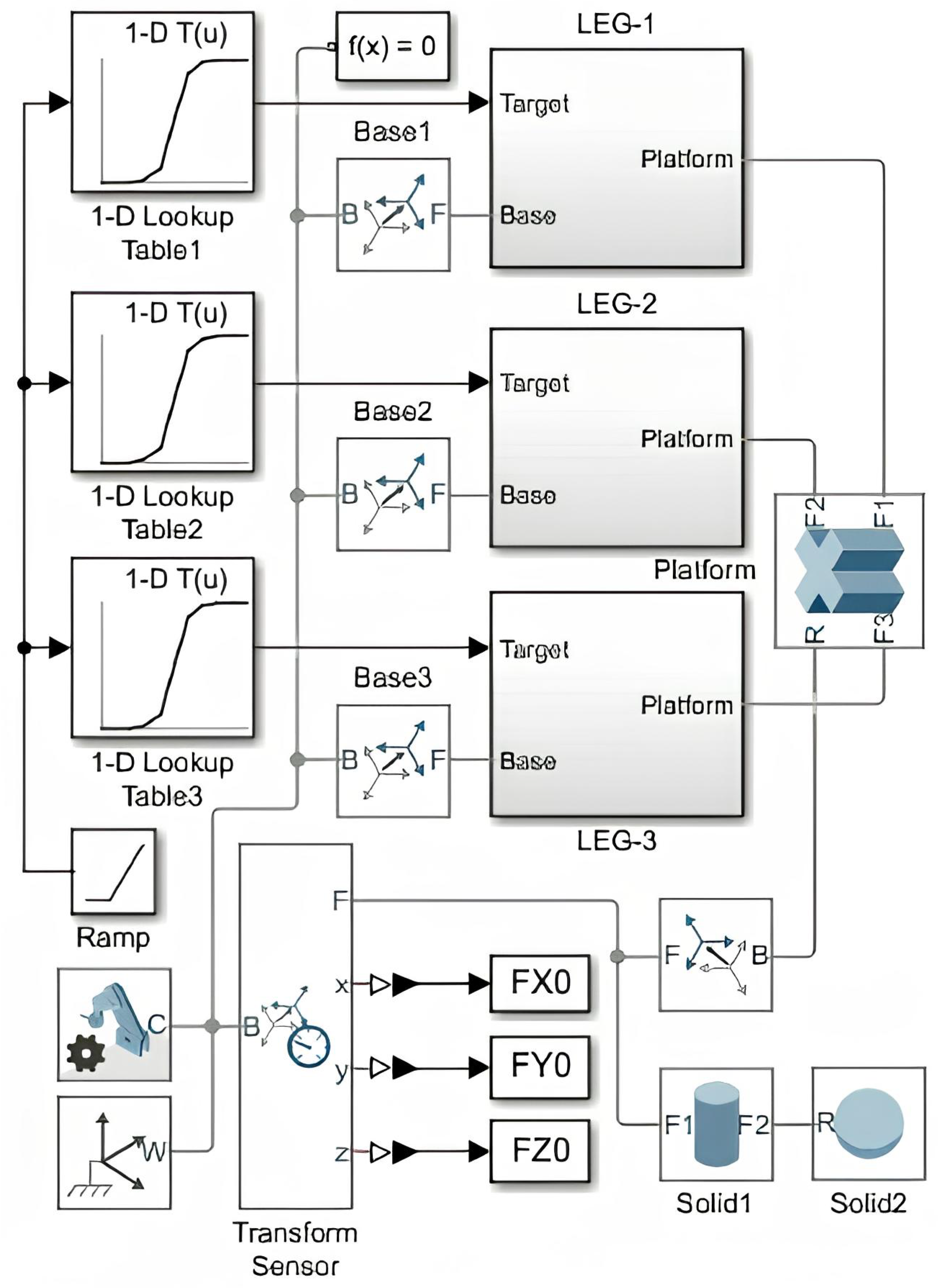
Delta robot model in MATLAB.
The model comprises three subsystems: LEG-1, LEG-2, and LEG-3, each containing parallel kinematic circuits connected to a fixed base and a movable platform. Each subsystem also includes a target input, which receives the current setting of the corresponding angle .
Motion settings from a precalculated trajectory are sequentially supplied. For subsequent analysis of the control results, the transform sensor stores a retrospective record of the moving platform’s positions. Solid blocks model the tip of the dosing device.
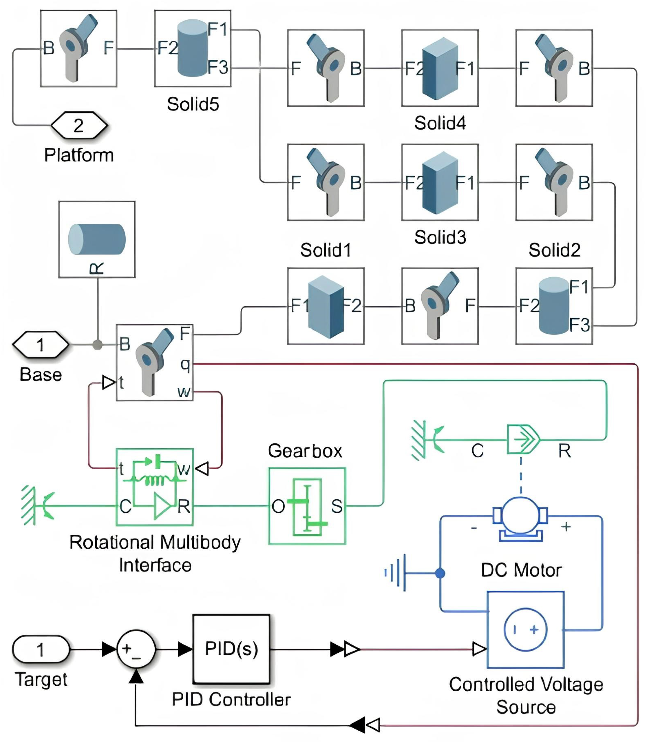
The contents of the subsystems are identical (Figure 24). Each subsystem includes the kinematic chain itself (the Solid1 rod and parallelogram joint—the remaining solid blocks with all necessary joints), a DC motor with a gearbox, a device for matching angular velocity and torque (rotational multibody interface), a controlled stress source, and a closed-loop system for the automatic control of the drive joint rotation angle with a PID controller. Electric motors with the following parameters are used as drive motors in the model: rated supply voltage, 12 V; rated load (mechanical power), 10 W; anchor inductance, 0.01 Gn; rotor inertia, 0.0002 ; rotor damping, (rad/s); rated rotation speed (at rated load), 2500 rpm. The geometric parameters of the robot were selected in accordance with the physical model GSK c4-1100. The kinematic chain is depicted in gray, the electrical components in blue, the mechanical parts in green, the control system in black, and the physical signals in brown.

Figure 24.
LEG-1 subsystem.
To ensure the sustainability of the control system, its stability was assessed. Since the inertia-free modules (trajectory estimation and mobile platform in Figure 22 do not influence the stability of the control system, the assessment is restricted to determining the stability of three identical automatic rotation angle control loops. During the identification of the unchangeable parts of the circuit, which includes an electric motor, a gearbox, a control object in the form of a rotary joint, and a rotation angle sensor, it was found that the control system is nonlinear. This is because the load on the electric motor shaft varies significantly depending on the position of the delta robot. Consequently, the Popov criterion was employed to verify its stability. As a result of this analysis, constraints were established for the controller parameters, ensuring the stability of the control system.
The following accuracy limits have been set for the robotic system: during the interaction, the dynamic error of the delta robot in the (x, y) plane should not exceed 1 mm to ensure that the pipette remains properly aligned within the test tube; during aspiration, the error along the z-axis should not exceed 0.2 mm.
During the simulation, the fulfillment of these restrictions was directly validated. The limitations were formulated with some margin based on the accuracy characteristics of the second element of the robotic system, the serial robot, which utilizes the AUBO-i5 manipulator [27]. The AUBO-i5 robot is constructed using a mechanism where straight and L-shaped elements are connected in a series through six driven rotary joints. Figure 25 illustrates its appearance and workspace, which is a spherical wedge of 350° with a coaxial cylindrical region removed from it.
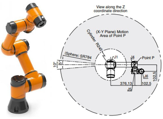
Figure 25.
AUBO-i5 manipulator and its workspace.
6.1. Interaction at the Point of Photographing
As mentioned in Section 1, if the delta robot is not delayed in reaching the interaction point, it is advisable to reduce the duration of the aliquoting cycle by minimizing the distance that the manipulator must slowly move the test tube containing biomaterial. To achieve this, it is recommended to conduct robot interaction directly at the tube photographing point. For the same reasons, it is also preferable to locate the photographing point near the rack with new test tubes.
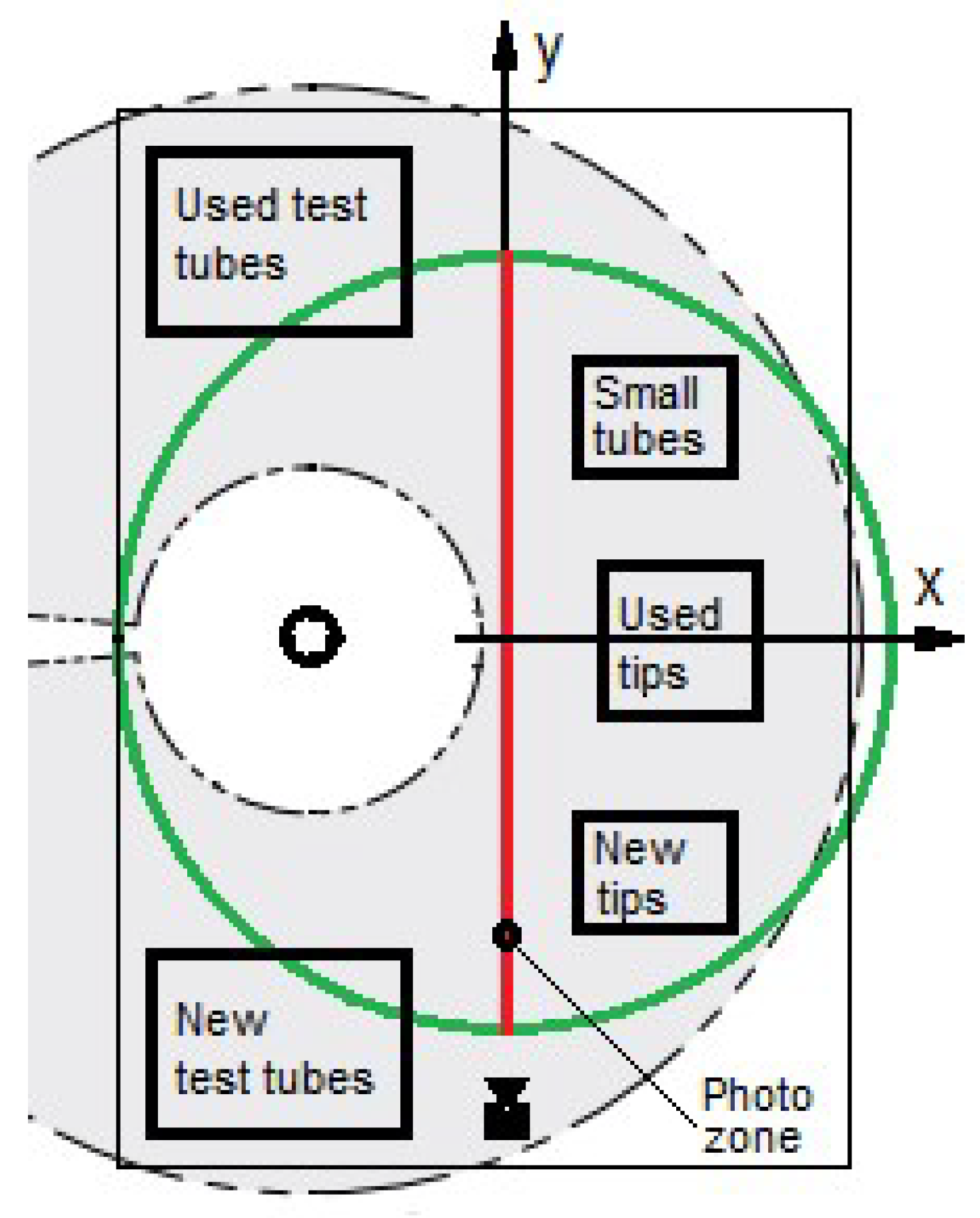
The proposed layout of the laboratory table, with approximate dimensions of 150 × 110 cm, provides for the installation of the serial robot in the center of the left half of the table (as shown in Figure 26) and the mounting of the delta robot above the center of the table. In the bottom-left corner of the figure is the new test tubes zone, where racks containing test tubes with biomaterial ready for aliquoting are placed. To the right is the photography area, used for imaging the test tubes. At the top-left is the used test tubes zone, where racks are installed to receive test tubes transported by the serial robot after biomaterial collection. On the right side of the table, the small tubes zone, used tips zone, and new tips zone are designated for the dosed dispensing of biomaterial into small tubes, removal of used tips, and installation of new tips, respectively. This arrangement enables the efficient organization of operations while accounting for the workspaces of each robot (the gray area corresponds to the serial robot’s workspace, and the area inside the green circle corresponds to the delta robot’s workspace). It can be observed from the drawing that it is convenient to organize interaction, for example, at one of the points along the red line. In this case, the manipulator can traverse this line (or its vicinity) in both directions: moving forward from the new test tubes zone through the photography area to the used test tubes zone while moving a test tube, and returning in the opposite direction to collect the next one. During the forward movement (upward in Figure 26), the delta robot can also follow the red line, return along an arc, and sequentially pass over the zones located on the right side of the table, from top to bottom.

Figure 26.
Layout of the laboratory table.
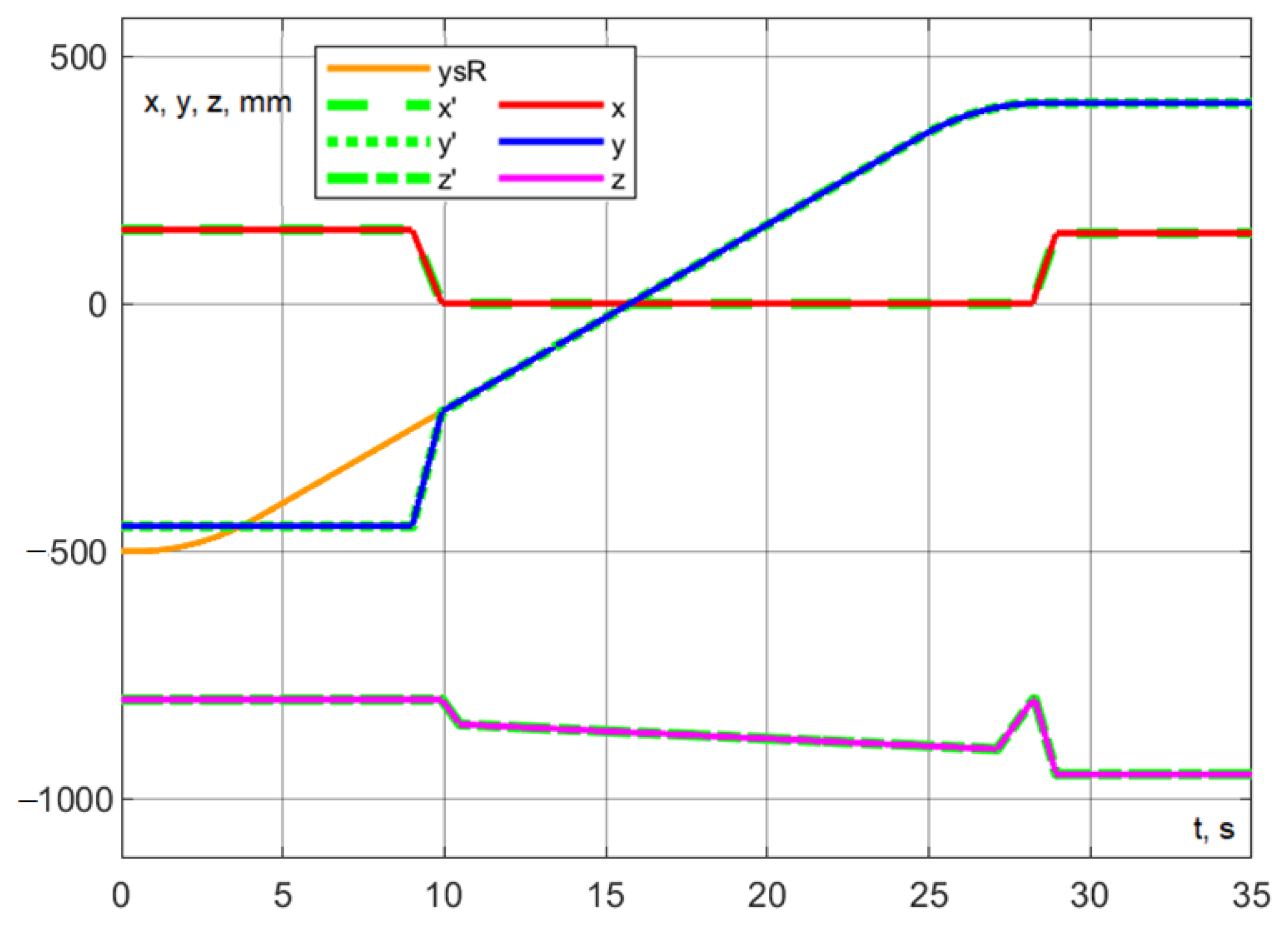
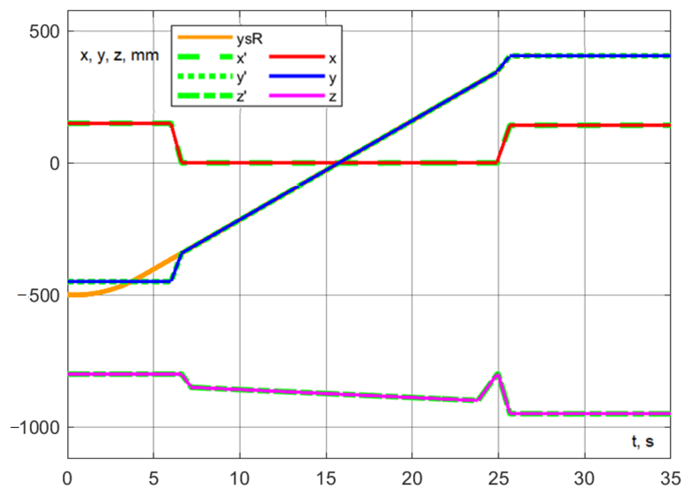
During the simulation, the trajectory of the delta robot’s movement corresponding to a portion of its working cycle was successfully executed. Figure 27 shows as the target coordinates and as the actual coordinate values.
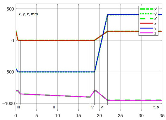
Figure 27.
Experiment No. 1. Practicing interaction at the point of photography.
The trajectory comprises the following stages: moving the tip of the dosing device from the installation area to the photography area (section I in Figure 27, velocity = 300 mm/s), followed by a slow lowering (section III, velocity = 90 mm/s), followed by a slow lowering (section III, velocity = 3 mm/s), removing the pipette (section IV, velocity = 90 mm/s), and moving to the dosing area while simultaneously lowering the pipette (section V, velocity = 300 mm/s). The entire trajectory is completed in 21.94 s.
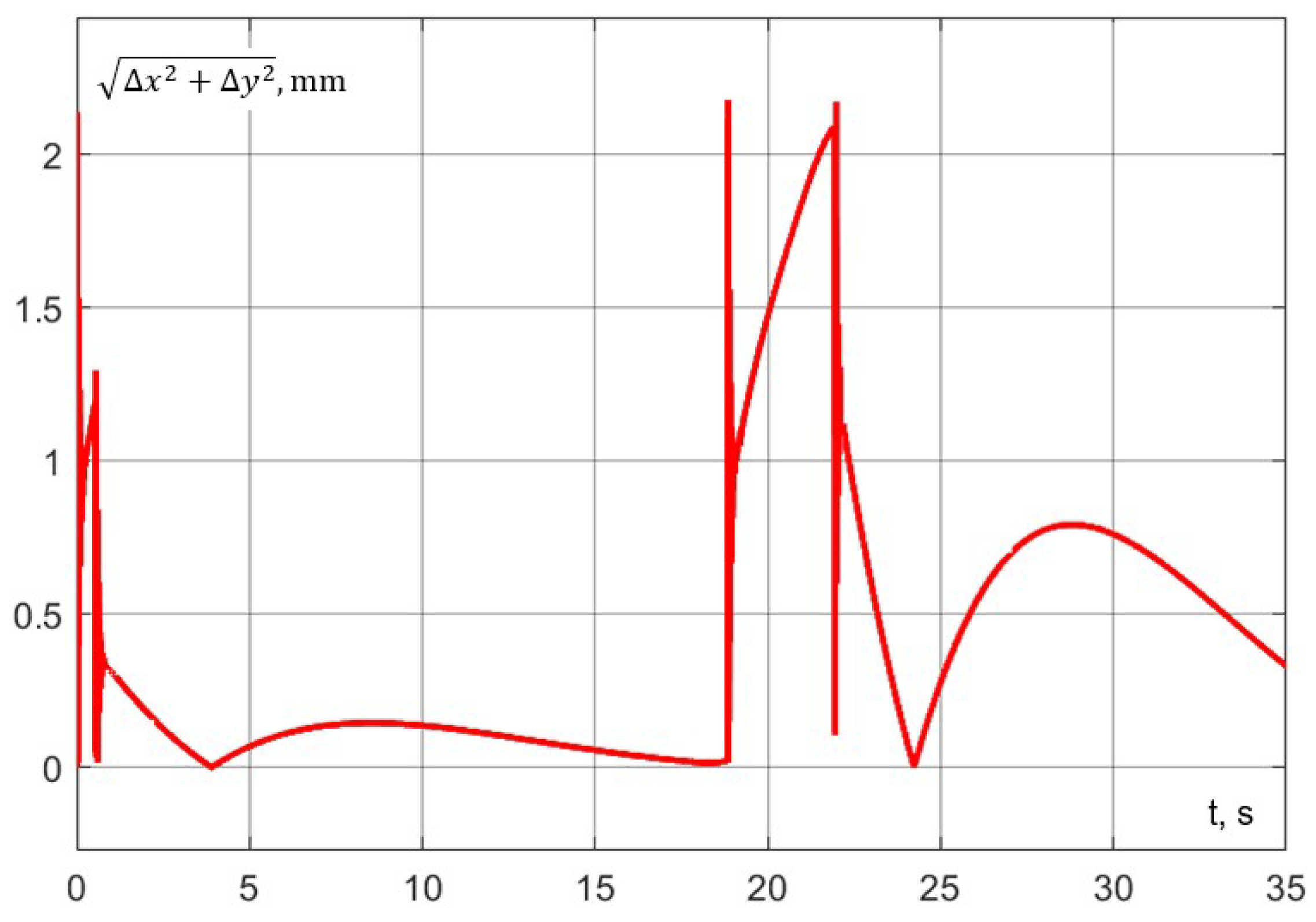
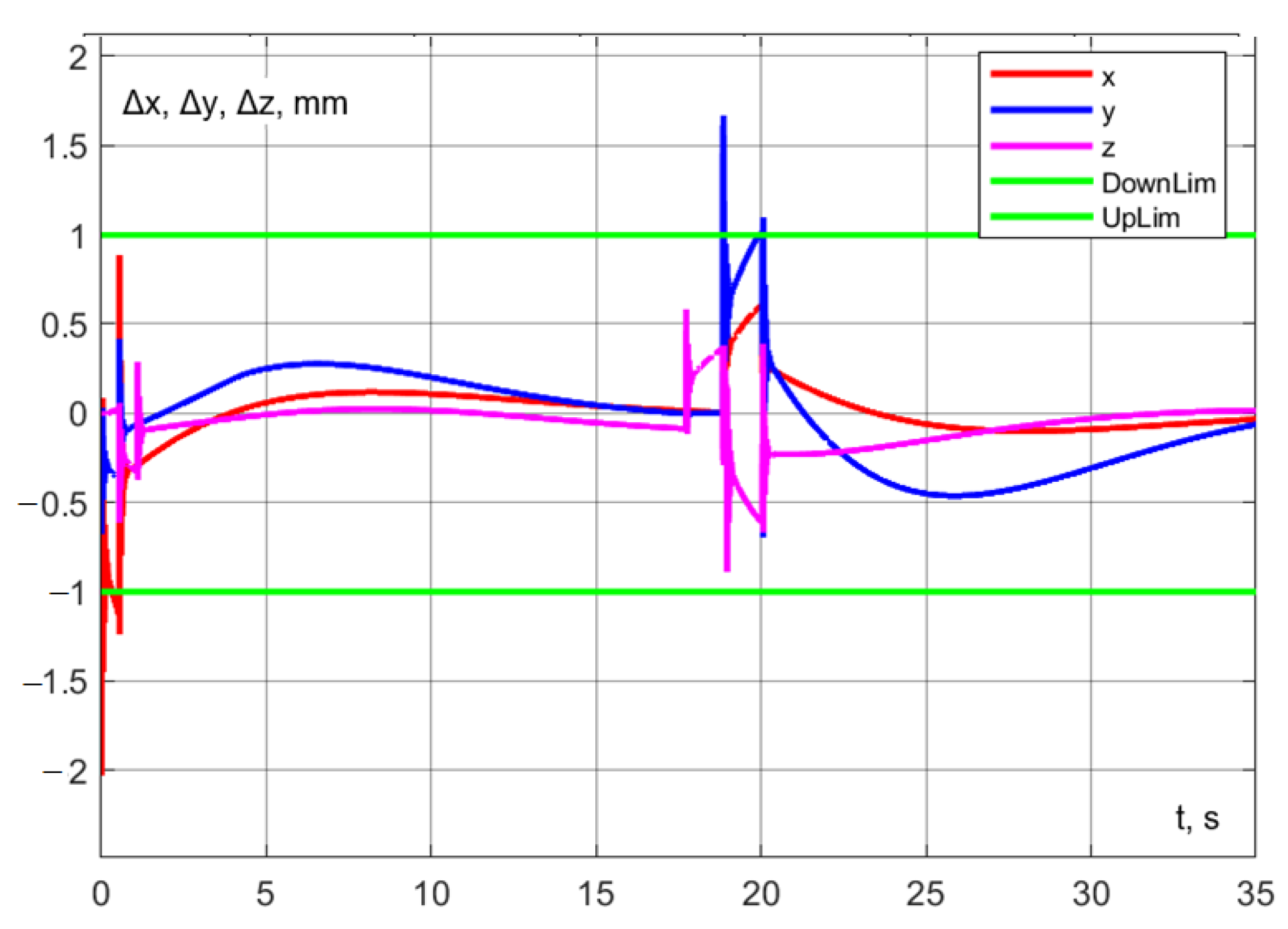
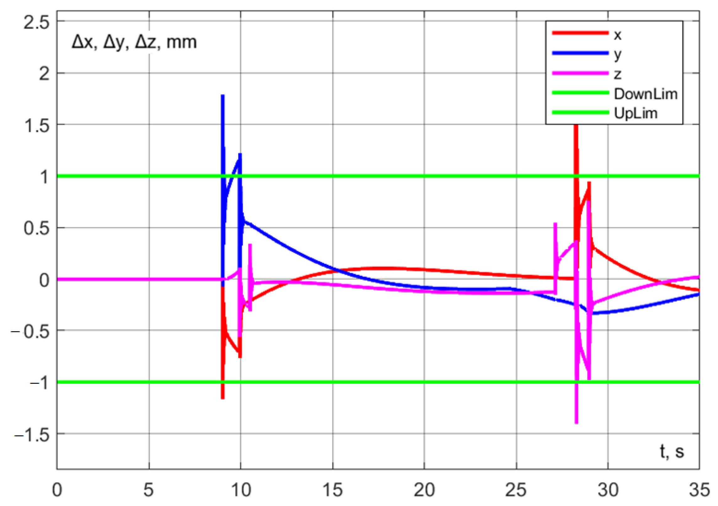
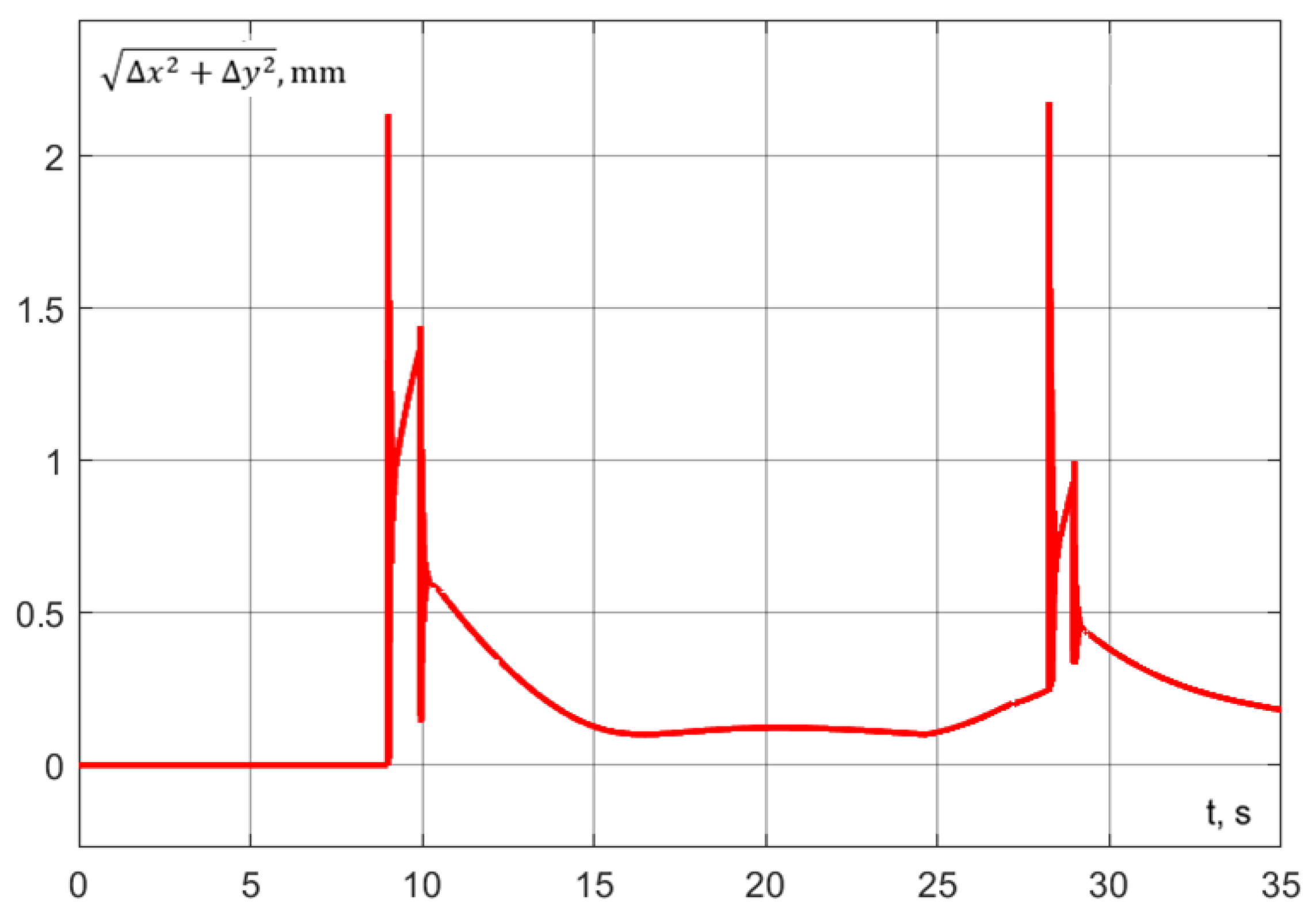
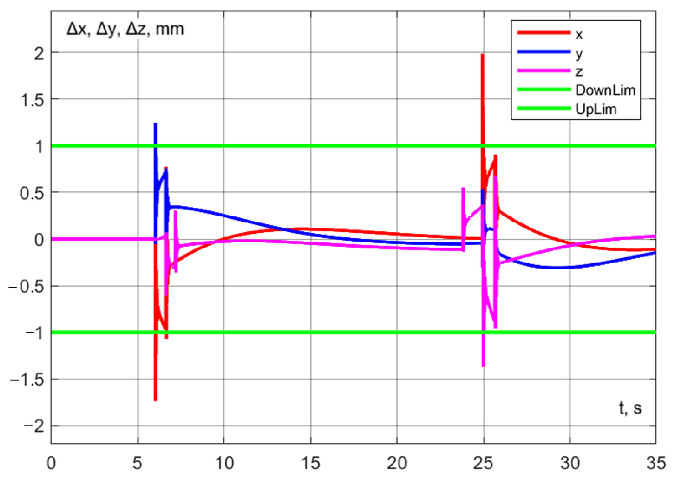
The accuracy of trajectory execution can be assessed from the dynamic error graph (Figure 28). Notably, the error along the z-axis during aspiration remains within 0.2 mm. Additionally, the dynamic error in the () plane during robot interaction does not exceed 1 mm (Figure 29).
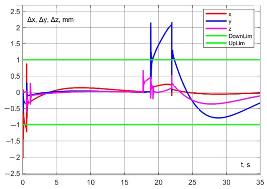
Figure 28.
Experiment No. 1. Dynamic error on coordinate axes.
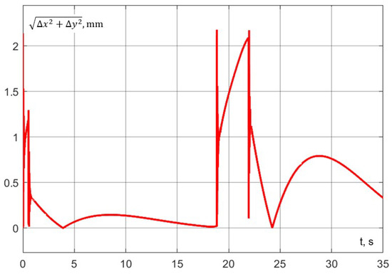
Figure 29.
Experiment No. 1. Dynamic error in the plane ().
Now let us assume that, as a result of determining the liquid levels in the test tube, it became known that the delta robot would be 9 s late for the next stage of interaction. If nothing is changed, this time will simply be lost, and the total duration of working out the trajectory will be 21.94 + 9 = 30.94 s. If you change the point of interaction, you can spend an additional 9 s approaching the dosing site and the rack with spent test tubes and thus save a little time.
6.2. Transferring an Interaction Point
Thus, the interaction point is shifted along the y-axis (it lies on the red segment in Figure 25 above the photography point). As noted in Section 1, the test tube containing liquid must be moved carefully to avoid inducing fluctuations. To achieve this, it is necessary to limit the acceleration at which the serial robot begins and ends its movement.
To cover the biggest possible distance, the test tube should move from the photography point to the new interaction point in two stages: the first stage involves moving half of the distance at an equidistant acceleration, and the second stage involves moving the remaining half with the same magnitude of acceleration. If the velocity on any segment of the trajectory exceeds the maximum permissible value, it is constrained to this limit. Upon being released, the delta robot proceeds to the interaction point at its maximum velocity. The robots must arrive at the interaction point simultaneously.
The most critical task is to determine the coordinates of the interaction point. Since the x and z coordinates of this point are known (the x coordinate is identical to that of the photography point, and the z coordinate corresponds to the position of the pipette above the test tube), the focus is on calculating the y coordinate, which is determined based on the following considerations:
- 1.
- During the movement of the delta robot, it traverses the distance from the starting point (, ) to the interaction point (0, y):where is the velocity of movement of the delta robot, is the time of its delay, and t is the time of movement of the serial robot.
- 2.
- For half the time of movement of the serial robot from the rest state (0, ), it covers half of the distance:where is the start time of the serial robot (the duration of segment I in Figure 27), is the moment in time when, starting from rest and accelerating at , the serial robot reaches its maximum permissible velocity.
To determine the interaction point of the robots, the following algorithm may be employed:
- Based on the analysis of the photographic image of the test tube, the levels of fraction separation and the number of aliquots are determined.
- One of two events is expected: either the insertion of the dosing device tip by the delta robot or the moving of a test tube to the photography area by the serial robot.
- If the installation of the dosing device tip is completed earlier than the moving test tube arrives at the photography zone, the photography point is designated as the interaction point, and the algorithm finishes.
- Considering the current position of the delta robot and the previously determined number of aliquots, the time required for it to reach the photography point is predictable.
- If the forecast indicates that there will be no delay with the delta robot, the photography point is assigned as the interaction point, and the algorithm finishes.
Substitute s, s, mm/s, mm/s, mm, mm, and mm. We assume mm/s2, which is 1000 times less than the gravitational acceleration, corresponds to the inclination of the test tube by = 0.057° = 3.4′ and, obviously, will not cause noticeable fluctuations in the liquid level.
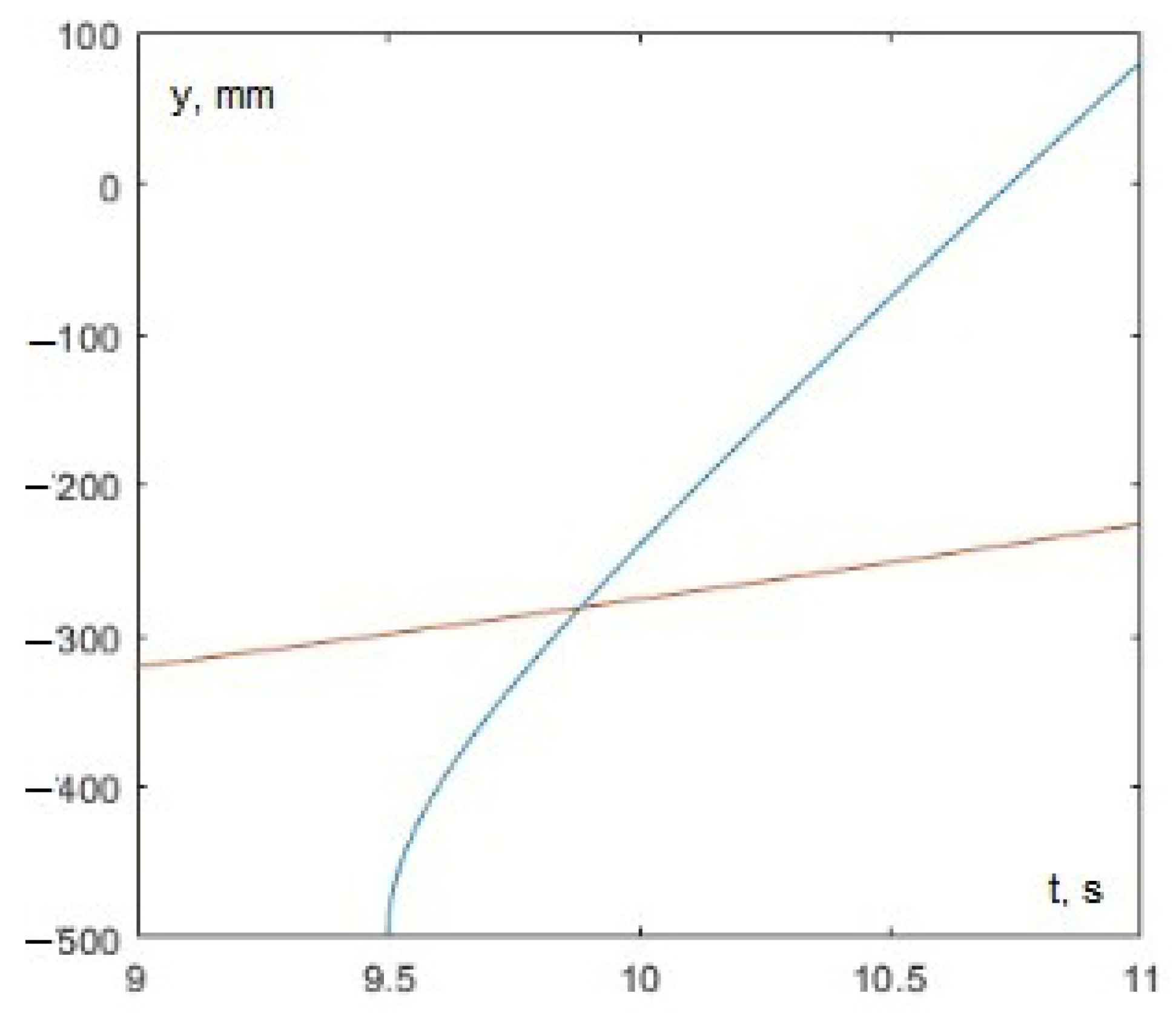
By jointly solving Equation (33) and system (34) using any acceptable method, the values s and mm are determined. The graphical solution is presented in Figure 30.

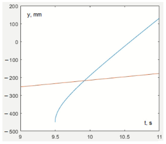
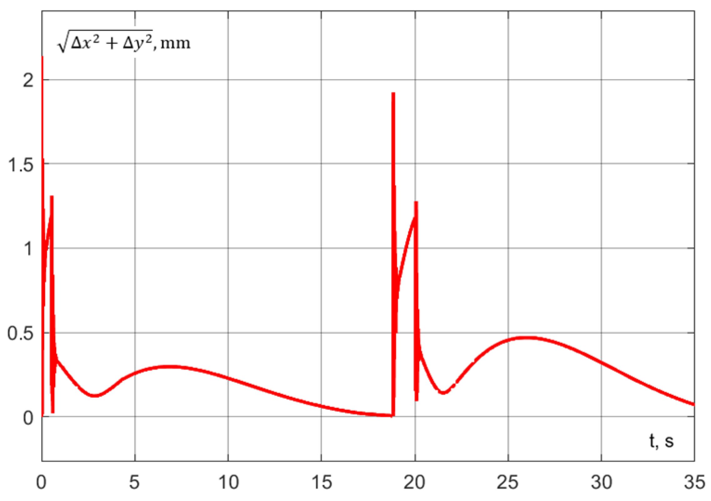
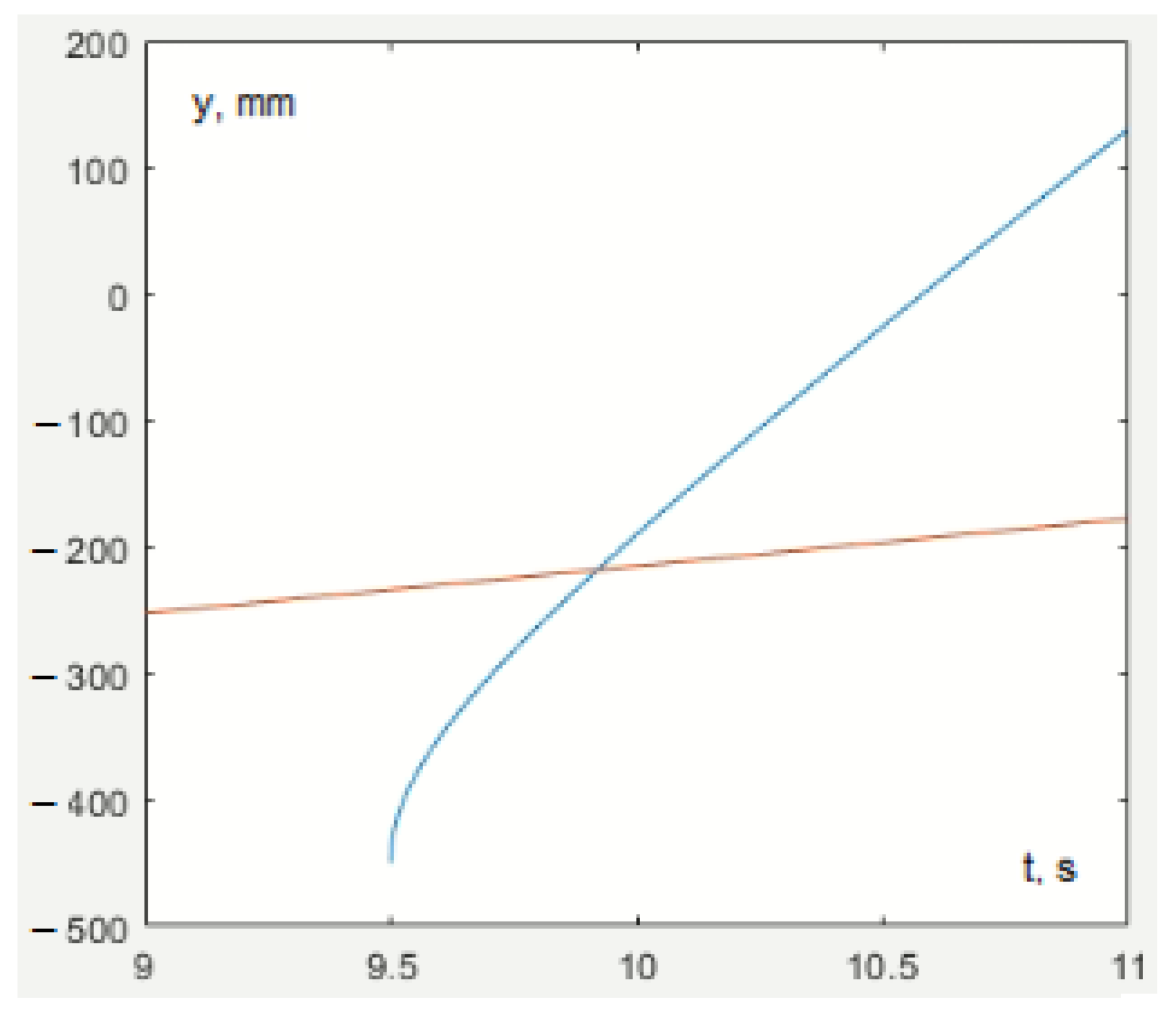
The corresponding trajectory was successfully executed (Figure 31). An additional orange line illustrates the change in the y coordinate of the serial robot until it converges with the delta robot.
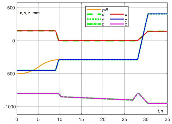
Figure 31.
Experiment No. 2. Working out interaction at the design point.
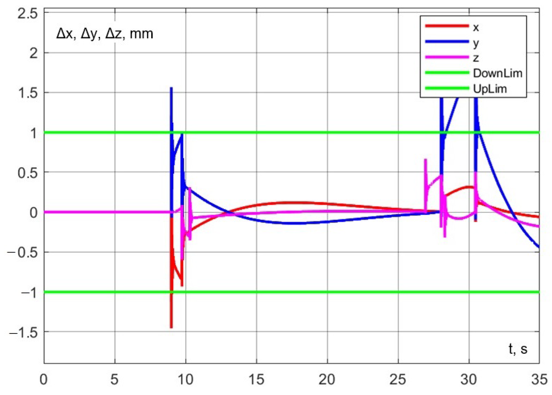
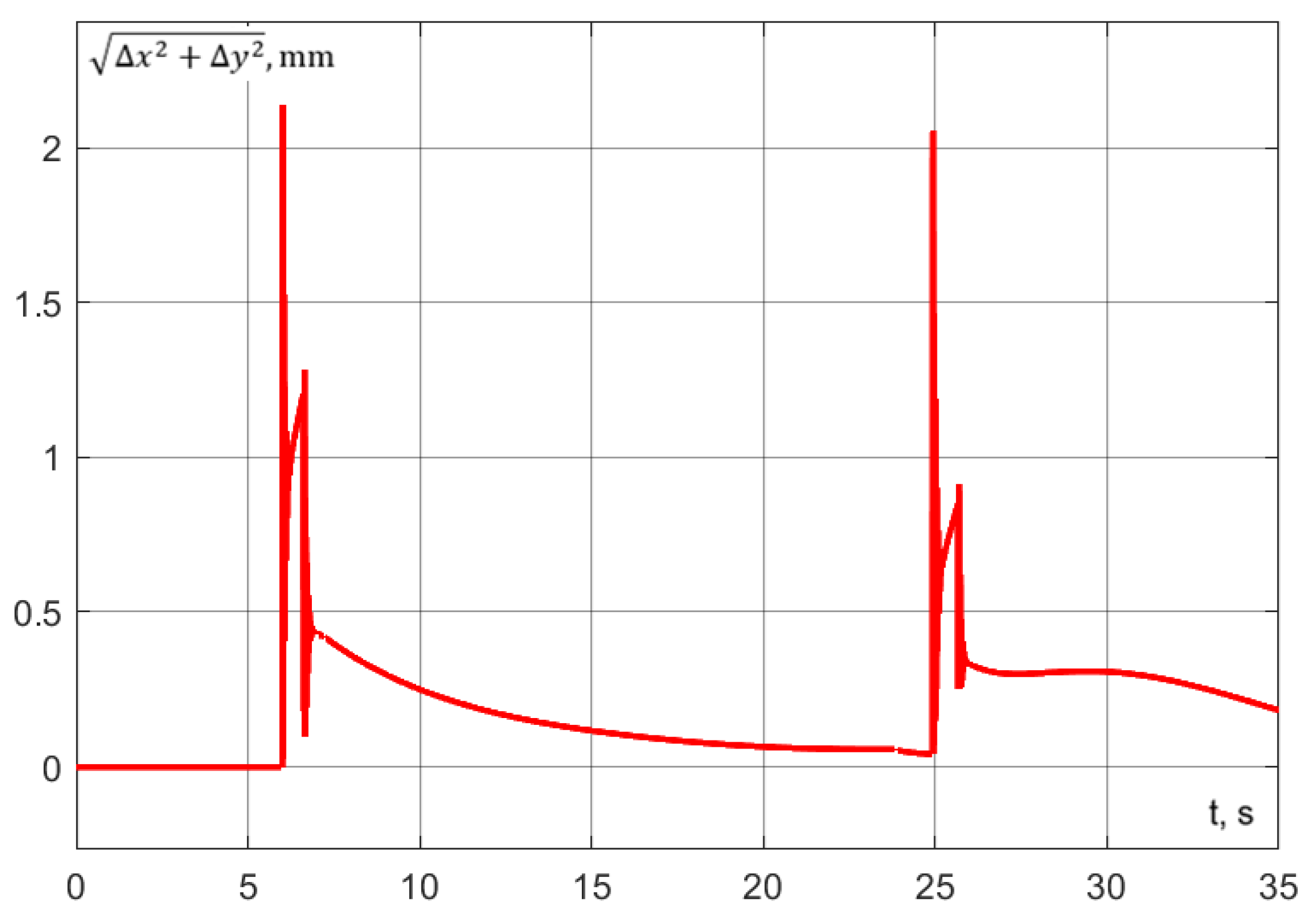
The accuracy of trajectory execution can be assessed from Figure 32 and Figure 33). As can be observed from the graphs, the error along the z-axis, as well as the error in the () plane, remains within the specified limits.

Figure 32.
Experiment No. 2. Dynamic error on coordinate axes.
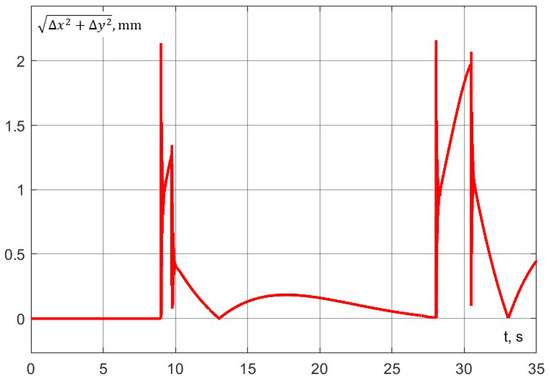
Figure 33.
Experiment No. 2. Dynamic error in the plane ().
The duration of the trajectory was 30.46 s, which is 0.48 s less than in the case of waiting at the photography point (Experiment 1). The relatively small time gain can be attributed to the fact that robot interaction in this robotic system takes significantly longer than their rapid movements, upon which the adaptation of the movement trajectory is based.
6.3. Interaction in Motion
An additional reduction in time can be achieved by organizing the interaction of robots during their movement. For the problem under investigation, this approach is quite feasible, provided that the constraint on the magnitude of the dynamic error is maintained.
Let us first consider the coordination of interaction during the motion, starting from the photography point. At some point in time as a pipette enters a test tube, a joint uniformly accelerated motion along the y-axis commences. Upon reaching the maximum allowable velocity, the motion along the y-axis continues at a constant speed until the pipette is completely withdrawn. Subsequently, the dosing device moves at maximum velocity toward the aliquoting site, while the test tube is directed to the rack for spent biomaterial.
The specified motion trajectory has been successfully executed (Figure 34) in 20.04 s, which is 1.90 s less than in the case where the interaction occurs entirely at the photography point (Experiment 1). A comparison with Figure 27 reveals that the time savings result from the reduction in segment V. From Figure 35 and Figure 36, it can be observed that the dynamic errors occurring during movement along this trajectory remain within the specified limits.
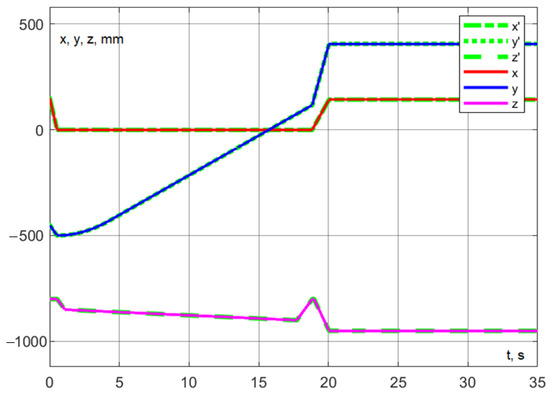
Figure 34.
Experiment No. 3. Practicing interaction in motion, starting at the point of photographing.

Figure 35.
Experiment No. 3. Dynamic error along the coordinate axes.
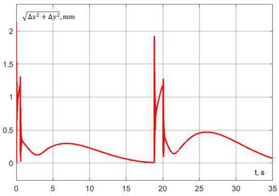
Figure 36.
Experiment No. 3. Dynamic error in plane ().
The described method of robot interaction during motion can be applied both when the delta robot arrives at the photography point on time and in the event of its delay. However, a delay in the delta robot’s arrival enables the combination of two time-saving approaches: robot interaction during motion and the relocation of their interaction point.
Thus, the serial robot moves the test tube from the photography point along the y-axis, first with uniform acceleration and then at a constant velocity. In contrast to the previously described case of relocating the interaction point, there is no need for the robot to stop at this point now.
Consequently, in the algorithm for calculating the interaction point, the system of Equation (32), is replaced with a system that determines the total path traversed by the serial robot to reach the interaction point:
Taking into account , expressing y, we obtain
By substituting the aforementioned values and solving Equation (33) and system (36) together, we determine the values s and mm (Figure 37).
The corresponding trajectory is presented in Figure 38, while the errors are shown in Figure 38, Figure 39 and Figure 40. The trajectory is completed in 28.94 s. This represents exactly a 2 s reduction compared to waiting for interaction at the photography point (Experiment 1) and a 1.52 s reduction compared to interacting at the calculated point (Experiment 2).
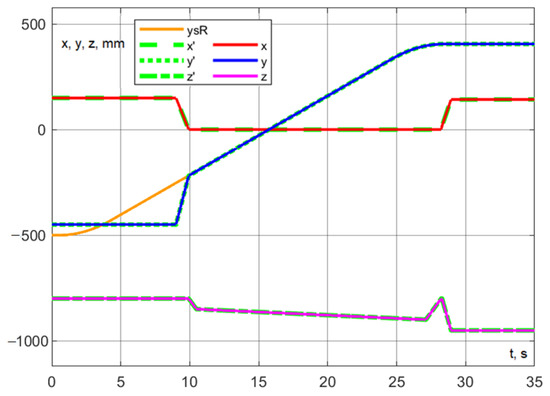
Figure 38.
Experiment No. 4. Development of interaction in motion, starting at the calculated point.
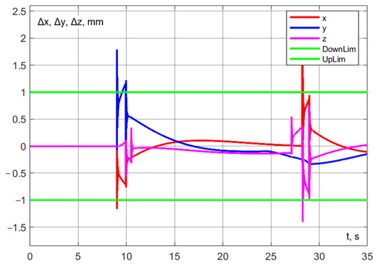
Figure 39.
Experiment No. 4. Dynamic error along the coordinate axes.
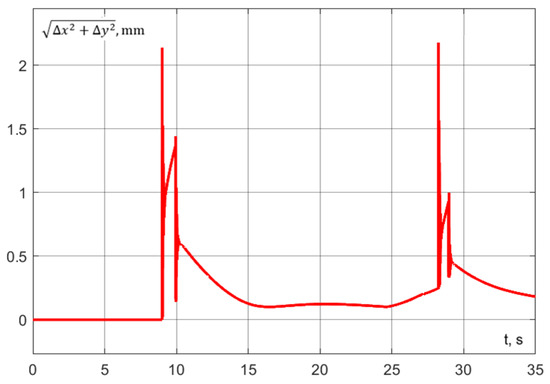
Figure 40.
Experiment No. 4. Dynamic error in plane ().
Compared to the scenario of interaction during motion starting at the photography point (Experiment 3), the advantage is significantly more modest. This is evidently due to the fact that the interaction did not fully occur within the segment of uniform motion (the linear portion of the graph in Figure 38), resulting in a segment of uniformly slow motion in Experiment 4.
When the delay is reduced to 6 s, robot interaction occurs along the straight segment depicted in Figure 41. Consequently, the time savings amount to 0.38 s relative to Experiment 3 and 2.28 s relative to Experiment 1, which corresponds to an approximate 9% increase in the operational efficiency of the robotic system.
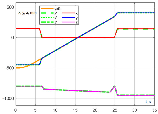
Figure 41.
Experiment No. 5. Development of interaction in motion with a delay of the delta robot by 6 s.
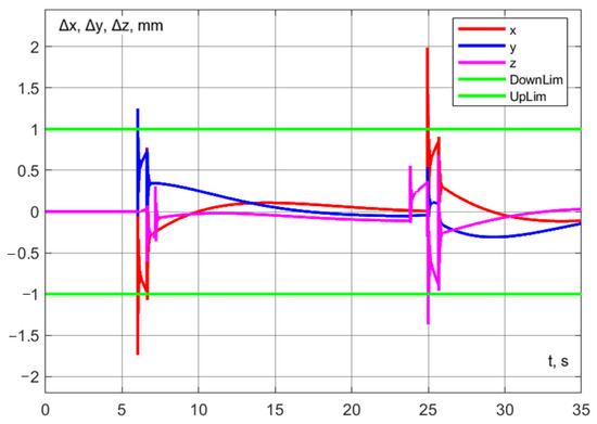
Figure 42.
Experiment No. 5. Dynamic error along the coordinate axes.
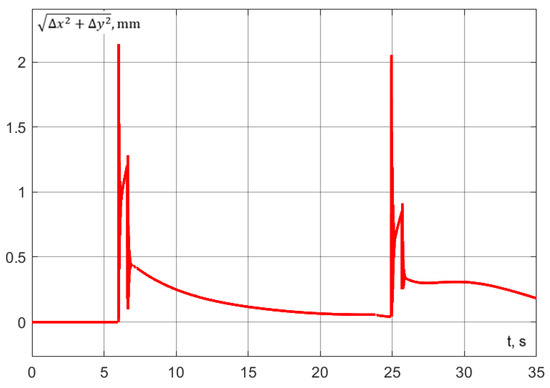
Figure 43.
Experiment No. 5. Dynamic error in plane ().
7. Conducting Experiments on Real Robots
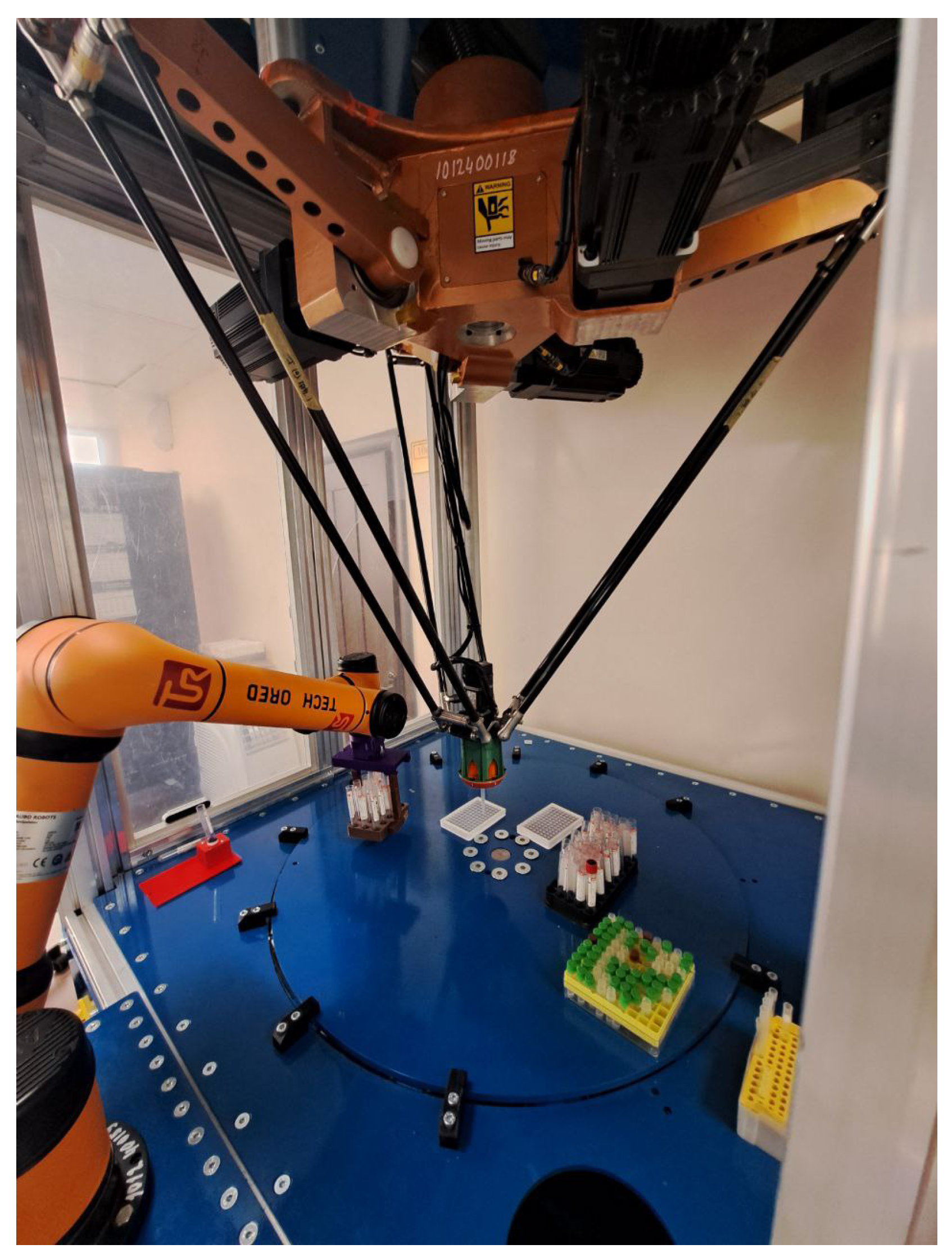
Experiments involving the biomaterial aliquoting process using the developed interaction algorithm were systematically reproduced on real robots. The absence of robot collisions during the aliquoting process in the limited areas defined in Section 5 was verified (Figure 44).

Figure 44.
Absence of robot intersections during aliquot operation.
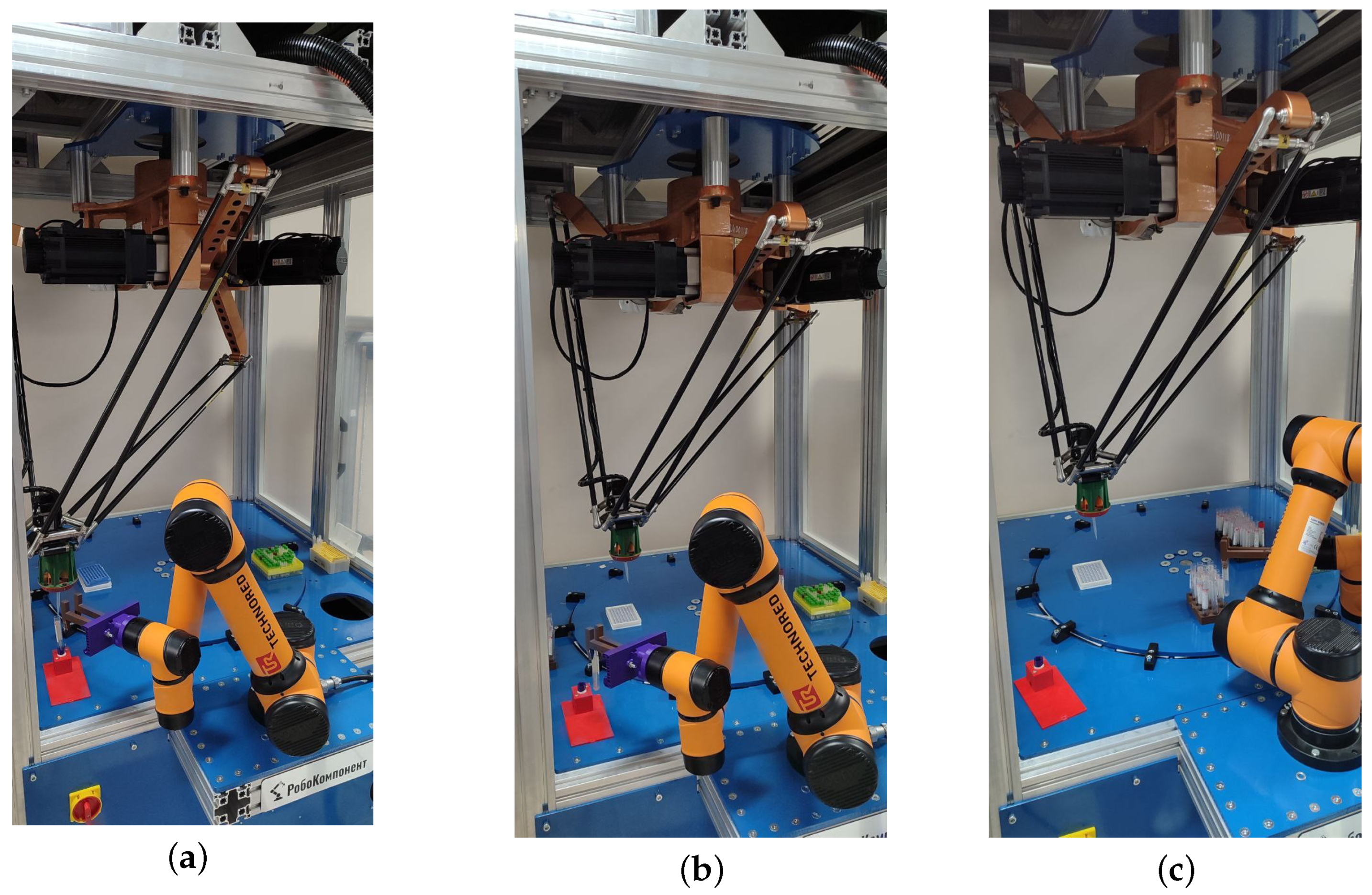
Experiments on real robots have shown that the estimate of the inertial characteristics of the delta robot’s electric drives, used to build its model in MATLAB, was somewhat overestimated. In addition, the requirements for the accuracy of the delta robot’s trajectory, adopted for mathematical modeling purposes with a certain margin, also turned out to be excessive. Their weakening made it possible to significantly increase the speed of movement of the robotic system; therefore, the duration of trajectory testing in the real system decreased in comparison with the model one. The control algorithm did not change: the rotation angle settings are still serially fed to the inputs of the local control circuits, in each of which the controller forms a control action on the electric drive; however, due to an increase in the speed of changing tasks, the performance of the algorithm increased, which is reflected in the results of the experiments. The delay time of the delta robot in Experiments 1–4 was set to 4 s. In the first experiment, robot interaction occurred at the photography point: the collaborative robot took a test tube containing a bio-sample, moved it to the photography point, and then the delta robot proceeded to the same point to acquire the tube. Following the simulation of liquid collection, the delta robot poured the sample into small tubes, while the collaborative robot placed the used test tube onto a rack. Under the conditions specified, the cycle duration was 11.1 s. Robot collaboration is illustrated in Figure 45.

Figure 45.
Performing a simulation of the fluid intake process at the point of photographing. (a) Liquid is drawn from the tube at the point of photographing; (b) the delta robot performs pipetting, and the collaborative robot performs the movement of the tube; (c) the delta robot continues pipetting, and the collaborative robot performs the capture of a new tube.
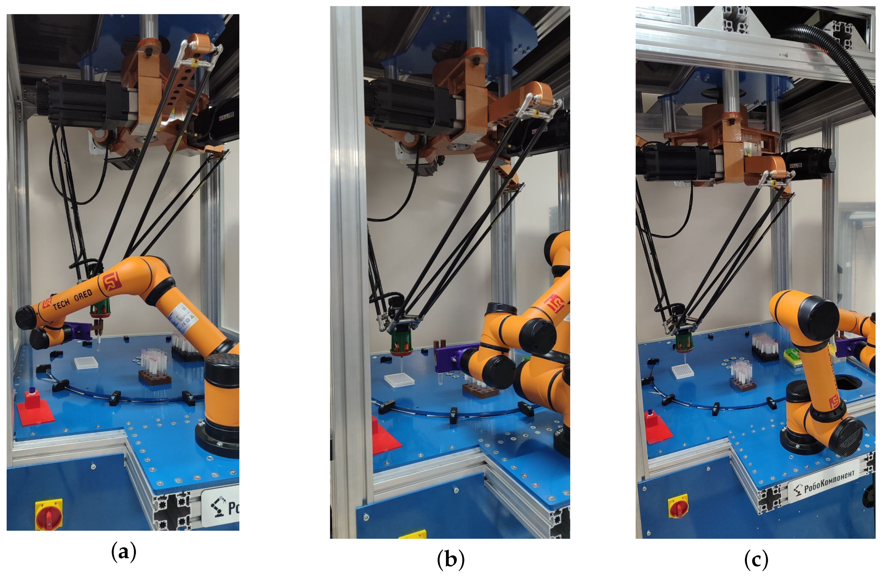
In Experiment No. 2, the robot interaction point was relocated along the y-axis, and its coordinates were determined by solving the system of Equation (34). Consequently, the cycle duration was reduced to 7.9 s, which represents a 28.1% decrease compared to that of Experiment No. 1. The movement of the robots in Experiment No. 2 is illustrated in Figure 46.
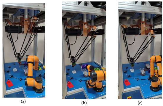
Figure 46.
Performing a simulation of the fluid intake process at the calculated interaction point. (a) Liquid is drawn from the test tube at the calculated point; (b) the delta robot performs pipetting, and the collaborative robot performs the movement of the tube; (c) the delta robot continues pipetting, and the collaborative robot places the used tube in a rack.
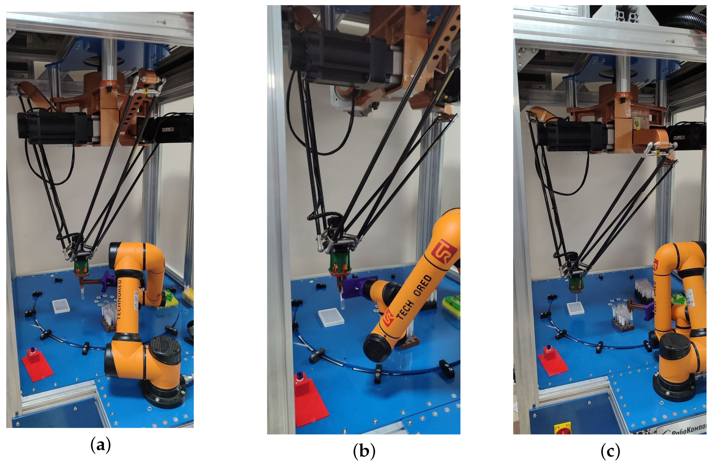
In Experiment No. 3, liquid sampling from a test tube was performed during the motion starting from the photography point. The cycle duration was 9.8 s, representing an 11.5% reduction compared to that of Experiment No. 1. The movement of the robots in Experiment No. 3 is illustrated in Figure 47.
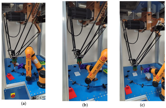
Figure 47.
Performing a simulation of fluid intake in motion from the point of photographing. (a) Fluid intake in motion from the point of photographing; (b) the end of fluid intake in motion; (c) the delta robot performs pipetting, and the collaborative robot moves the used tube.
In Experiment No. 4, the robot interaction point was relocated along the y-axis, and its coordinates were determined by solving the system of Equation (34). Unlike in Experiment No. 2, liquid intake was performed as the robots moved together from the calculated point along the y-axis. The cycle duration was 6.7 s, representing a 39.5% reduction compared to that of Experiment No. 1. The movement of the robots in Experiment No. 4 is illustrated in Figure 48.

Figure 48.
Performing a simulation of fluid intake in motion from a precalculated point. (a) Liquid intake in motion from the design point; (b) the delta robot performs pipetting, and the collaborative robot performs tube movement; (c) the delta robot continues pipetting, and the collaborative robot installs the used tube in a rack.
In Experiment No. 5, the delay time of the delta robot was decreased to 2 s, resulting in the interaction point being shifted along the y-axis. The cycle duration was 6.2 s, representing a 43.5% reduction compared to that of Experiment No. 1. The arrangement of the robots in this experiment is illustrated in Figure 49.
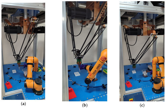
Figure 49.
Performing a simulation of fluid intake in motion from a precalculated point with a delta robot delay of 2 s. (a) Fluid intake in motion from the design point; (b) the end of fluid intake in motion; (c) the delta robot performs pipetting, and the collaborative robot moves the used tube.
To quantitatively evaluate the performance of the proposed control strategies, a series of 10 repeated experiments was conducted for each scenario. The execution time of the technological process was measured using a stopwatch with a resolution of 0.1 s. The results (Table 2) indicate that the average execution times across all scenarios were comparable, with variations within the measurement error margin (±0.2 s). This suggests that the considered control strategies exhibit similar efficiency in terms of process duration under the given experimental conditions.
Table 2.
Comparative analysis of system operation time in various scenarios.
While analyzing the experimental results, it was found that the cycle time for interaction at the precalculated point, combined with liquid intake simulation during motion and a delta robot delay of 4 s, was 6.7 s, which corresponds to a 39% reduction compared to the baseline experiment. With a delta robot delay of 2 s, the cycle time decreased to 6.2 s, representing a 43.5% improvement over the baseline experiment. The discrepancy in cycle time between simulations and experiments in real conditions occurs because the velocity characteristics of the robots and the actual object locations are not taken into account.
8. Conclusions
The algorithms developed allowed the organization of the relative position and the limitation of the areas of serial robot operation based on the exclusion of intersections of work safety zones for the specified ranges of motion. The volume of the permissible workspace of the end effector, taking into account the exclusion of collisions, decreased for each of the scenarios. For scenarios in which the delta robot is in the home position, the volume of the workspace of the serial robot decreased by 37.6%; for the scenario where the delta robot performs the aliquoting process, the volume decreased by 70.7%. The absence of robot collisions during the aliquoting process in the limited areas was verified in experiments.
Within the framework of this study, the potential for adapting the control algorithms of a robotic system to external disturbances—specifically, the workload of its components—was investigated with the aim of minimizing the processing time of a given trajectory. During the adaptation process, the robot trajectories were adjusted by selecting their interaction point and implementing interaction during the motion, ensuring that the accuracy characteristics of the robotic system remained unaffected.
Using the example of a robotic system for biomaterial aliquoting, it has been demonstrated that optimizing robot trajectories based on the proposed formal relationships enables the attainment of a certain reduction in the operating time of the robotic system while maintaining the specified positioning accuracy of its components. The maximum increase in the operational efficiency of the robotic system, as observed during the experiments compared to the baseline interaction mode of its elements, was approximately 43.5%.
In the course of the study, a delta robot was modeled using the MATLAB package. Graphs reflecting the accuracy of trajectory execution were obtained, a functional diagram of the control system was proposed, and an algorithm for determining the interaction point was developed.
During real robot experiments, it was found that, in Experiment No. 5, the cycle execution time was reduced by 43.5% compared to the baseline experiment, thereby confirming the feasibility and effectiveness of the developed algorithm.
Author Contributions
Conceptualization, S.K. and L.R.; methodology, L.R., S.K., and D.M.; software, D.M. and V.V.; validation, S.K. and L.R.; formal analysis, V.V. and V.C.; investigation, S.K., D.M., V.V., and V.C.; resources, L.R.; data curation, L.R. and S.K.; writing—initial draft preparation, V.V.; writing—review and editing, V.C. and S.K.; visualization, D.M. and V.C.; supervision, L.R.; project administration, L.R.; funding acquisition, L.R. All authors have read and agreed with the published version of the manuscript.
Funding
This research was supported by a state assignment of the Ministry of Science and Higher Education of the Russian Federation under grant FZWN-2020-0017.
Data Availability Statement
The original contributions presented in this study are included in the article. Further inquiries can be directed to the corresponding authors.
Conflicts of Interest
The authors declare no conflicts of interest.
References
- Tarbouriech, S.; Navarro, B.; Fraisse, P.; Crosnier, A.; Cherubini, A.; Salle, D. Admittance control for collaborative dual-arm manipulation. In Proceedings of the 19th International Conference on Advanced Robotics, Belo Horizonte, Brazil, 2–6 December 2019; Volume 8981624, pp. 198–204. [Google Scholar]
- Huang, C.; Zhou, S.; Li, J.; Radwin, R. Allocating Robots/Cobots to Production Systems for Productivity and Ergonomics Optimization. IEEE Trans. Autom. Sci. Eng. 2023, 21, 2841–2855. [Google Scholar] [CrossRef]
- Desai, J.P.; Ostrowski, J.; Kumar, V. Controlling formations of multiple mobile robots. In Proceedings of the IEEE International Conference on Robotics and Automation, Leuven, Belgium, 20–20 May 1998; Volume 4, pp. 2864–2869. [Google Scholar]
- Lewis, M.A.; Tan, K.H. High precision formation control of mobile robots using virtual structures. Auton. Robots 1997, 4, 387–403. [Google Scholar] [CrossRef]
- Sandeep, S.; Fidan, B.; Yu, C. Decentralized cohesive motion control of multi-agent formations. In Proceedings of the 14th Mediterranean Conference on Control and Automation, Ancona, Italy, 28–30 June 2006; pp. 1–6. [Google Scholar]
- Olfati-Saber, R.; Murray, R.M. Distributed cooperative control of multiple vehicle formations using structural potential functions. IFAC Proc. 2002, 15, 242–248. [Google Scholar] [CrossRef]
- Balch, T.; Arkin, R.C. Behavior-based formation control for multi robot teams. Robotics and Automation. IEEE Trans. 1998, 14, 926–939. [Google Scholar]
- Eren, T.; Belhumeur, P.N.; Anderson, B.D.; Morse, A.S. A framework for maintaining formations based on rigidity. In Proceedings of the 15th IFAC World Congress, Barcelona, Spain, 21–26 July 2002; pp. 2752–2757. [Google Scholar]
- Areak, M. Passivity as a design tool for group coordination. In Proceedings of the IEEE American Control Conference, Minneapolis, MN, USA, 14–16 June 2006; p. 6. [Google Scholar]
- Wang, C.; Xie, G.; Cao, M. Forming circle formations of anonymous mobile agents with order preservation. IEEE Trans. Autom. Control 2013, 58, 3248–3254. [Google Scholar] [CrossRef]
- Ferber, J. Multi-Agent Systems an Introduction to Distributed Artificial Intelligence; Addison-Wesley Reading: Boston, MA, USA, 1999; Volume 1. [Google Scholar]
- Buhla, J.F.; Gronhoj, R.; Jorgensen, J.K.; Mateus, G.; Pinto, D.; Sorensen, J.K.; Bogh, S.; Chrysostomou, D. A Dual-arm Collaborative Robot System for the Smart Factories of the Future. Procedia Manuf. 2019, 38, 333–340. [Google Scholar] [CrossRef]
- Yan, L.; Stouraitis, T.; Vijayakumar, S. Decentralized Ability-Aware Adaptive Control for Multi-Robot Collaborative Manipulation. IEEE Robot. Autom. Lett. 2021, 6, 2311–2318. [Google Scholar] [CrossRef]
- Wang, M. Adaptive Control Strategy for Robot Motion Planning in Complex Environments. Sci. J. Intell. Syst. Res. 2024, 6, 1–5. [Google Scholar] [CrossRef]
- Xiao, F.; Li, B.; Huang, H.; Xi, F. Obstacle Avoidance of Multiple Manipulators Based on 3D Artificial Potential Field Method. In Proceedings of the 2021 IEEE 11th Annual International Conference on CYBER Technology in Automation, Control, and Intelligent Systems, Jiaxing, China, 27–31 July 2021; pp. 198–203. [Google Scholar]
- Guclu, E.; Örnek, Ö.; Ozkan, M.; Yazici, A.; Demirci, Z. An Online Distance Tracker for Verification of Robotic Systems Safety. Sensors 2023, 23, 2986. [Google Scholar] [CrossRef]
- Rana, A.S.; Zalzala, A.M.S. Near Time-Optimal Collision-Free Motion Planning of Robotic Manipulators Using an Evolutionary Algorithm. Robotica 1996, 14, 621–632. [Google Scholar] [CrossRef]
- Yang, L.; Li, P.; Wang, T.; Miao, J.; Tian, J.; Chen, C.; Tan, J.; Wang, Z. Multi-area collision-free path planning and efficient task scheduling optimization for autonomous agricultural robots. Sci. Rep. 2024, 14, 18347. [Google Scholar] [CrossRef] [PubMed]
- Di Castro, M.; Mulero, D.B.; Ferre, M.; Masi, A. Real-time reconfigurable collision avoidance system for robot manipulation. In Proceedings of the 3rd International Conference on Mechatronics and Robotics Engineering, Paris, France, 8–12 February 2017; Volume F128050, pp. 6–10. [Google Scholar]
- Sharkawy, A.-N.; Koustoumpardis, P.N.; Aspragathos, N.A. Manipulator collision detection and collided link identification based on neural networks. Mech. Mach. Sci. 2019, 67, 3–12. [Google Scholar]
- Rosenfeld, A.; Kaminka, G.; Kraus, S. Adaptive Robot Coordination Using Interference Metrics. In Proceedings of the 16th European Conference on Artificial Intelligence, Valencia, Spain, 22–27 August 2004; pp. 910–916. [Google Scholar]
- Malyshev, D.; Rybak, L.; Carbone, G.; Semenenko, T.; Nozdracheva, A. Optimal Design of a Parallel Manipulator for Aliquoting of Biomaterials Considering Workspace and Singularity Zones. Appl. Sci. 2022, 12, 2070. [Google Scholar] [CrossRef]
- The Delta Parallel Robot. Kinematics Solutions. Available online: https://people.ohio.edu/williams/html/PDF/DeltaKin.pdf (accessed on 9 April 2025).
- Rybak, L.; Cherkasov, V.; Malyshev, D.; Diakonov, D.; Carbone, G. New Design of the Gripper and Its Orientation Algorithm for Placing Test Tubes and Racks with a Robotic System for Aliquoting Bio-materials. Mech. Mach. Sci. 2024, 165, 192–203. [Google Scholar]
- Rybak, L.; Carbone, G.; Malyshev, D.; Nozdracheva, A.; Dyakonov, D.; Cherkasov, V. Algorithms for Determinating the Work Safety Zones of Manipulators of Various Structures as Part of a Multi-The Robotic System. I4SDG 2025, 2021; submitted. [Google Scholar]
- Behera, L.; Rybak, L.; Malyshev, D.; Gaponenko, E. Determination of Workspaces and Intersections of Robot Links in a Multi-Robotic System for Trajectory Planning. Appl. Sci. 2021, 11, 4961. [Google Scholar] [CrossRef]
- AUBO-i5. Collaborative Lightweight Robot. Available online: https://www.netetrade.com/media/aubo-robotics-usa/files/5c7b8264-6b52-4e59-b4c2-a8fc7d6233f8.pdf (accessed on 9 April 2025).


Disclaimer/Publisher’s Note: The statements, opinions and data contained in all publications are solely those of the individual author(s) and contributor(s) and not of MDPI and/or the editor(s). MDPI and/or the editor(s) disclaim responsibility for any injury to people or property resulting from any ideas, methods, instructions or products referred to in the content. |
© 2025 by the authors. Licensee MDPI, Basel, Switzerland. This article is an open access article distributed under the terms and conditions of the Creative Commons Attribution (CC BY) license (https://creativecommons.org/licenses/by/4.0/).