
Attempts at Pseudo-Inverse Vibro-Acoustics by Means of SLDV-Based Full-Field Mobilities


Abstract
1. Introduction
2. Materials and Methods
2.1. Full-Field SLDV Mobilities from the TEFFMA Project
2.1.1. Characterisation of the Structural Dynamics by Means of Full-Field Mobilities
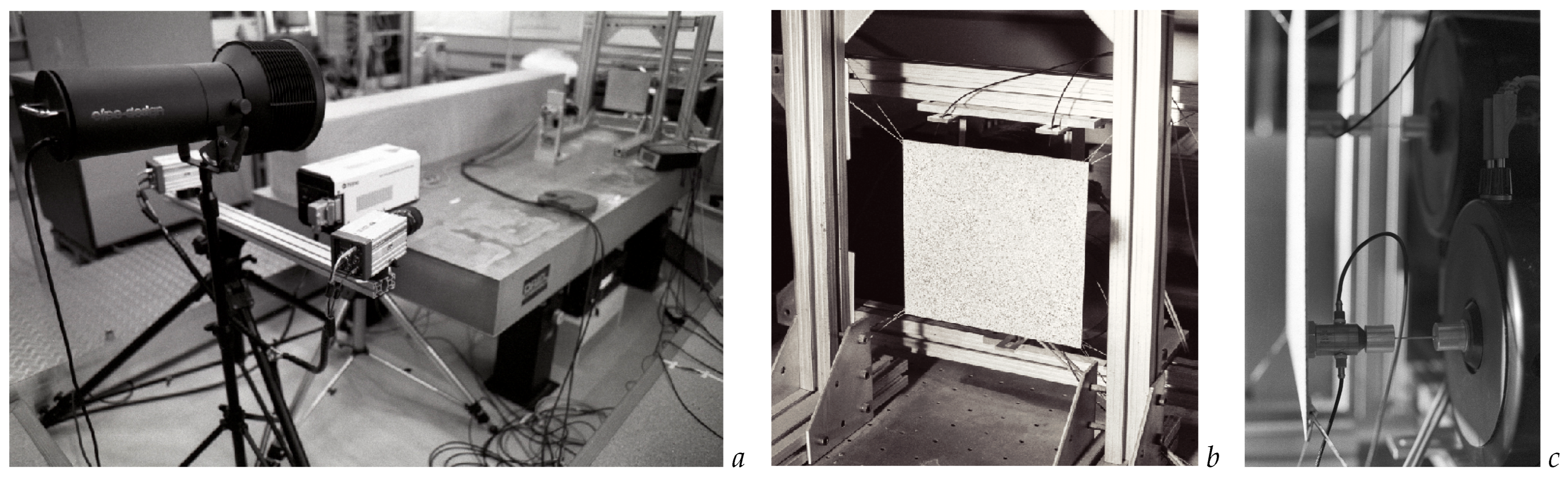
2.1.2. Brief Notes About the Tested Plate in the TEFFMA Project
2.1.3. Notes on the Processing of the Full-Field Mobilities
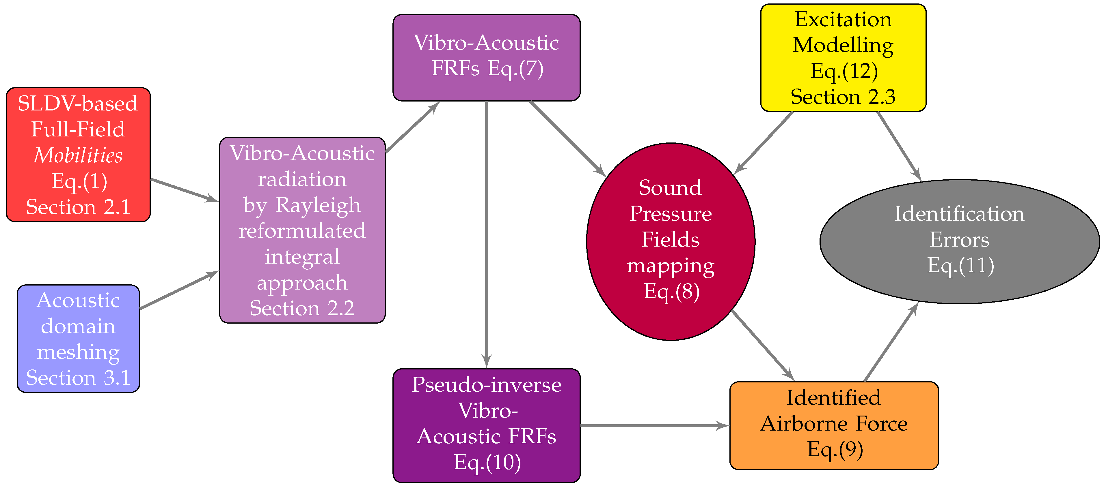
2.2. Simplified Formulation for Direct and Pseudo-Inverse Vibro-Acoustics
2.2.1. Sound Pressures in a Direct Formulation of Vibro-Acoustics by Full-Field Mobilities
2.2.2. Induced Forces in a Pseudo-Inverse Formulation of Vibro-Acoustics by Full-Field Mobilities
2.3. Simple Broad Frequency Band Modelling of the Excitation Forces
Complex-Valued Coloured Noise with Random Amplitude and Phase Variations
3. Results

| Section | Equation | Quantity | Acoustic Domain, | Structural | Frequency | Figure |
|---|---|---|---|---|---|---|
| Excitation | Domain | Domain | ||||
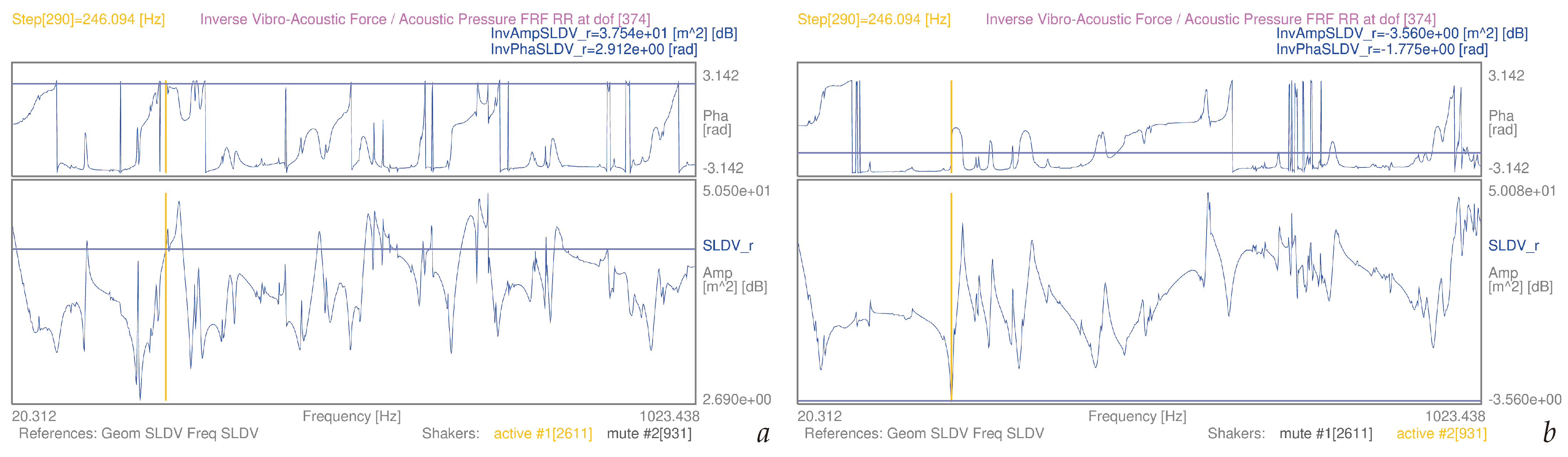
| 3.4 | (10) | single dof [374], – | S1 | [20–1024] Hz | 11a | |
| 3.4 | (10) | single dof [374], – | S2 | [20–1024] Hz | 11b | |
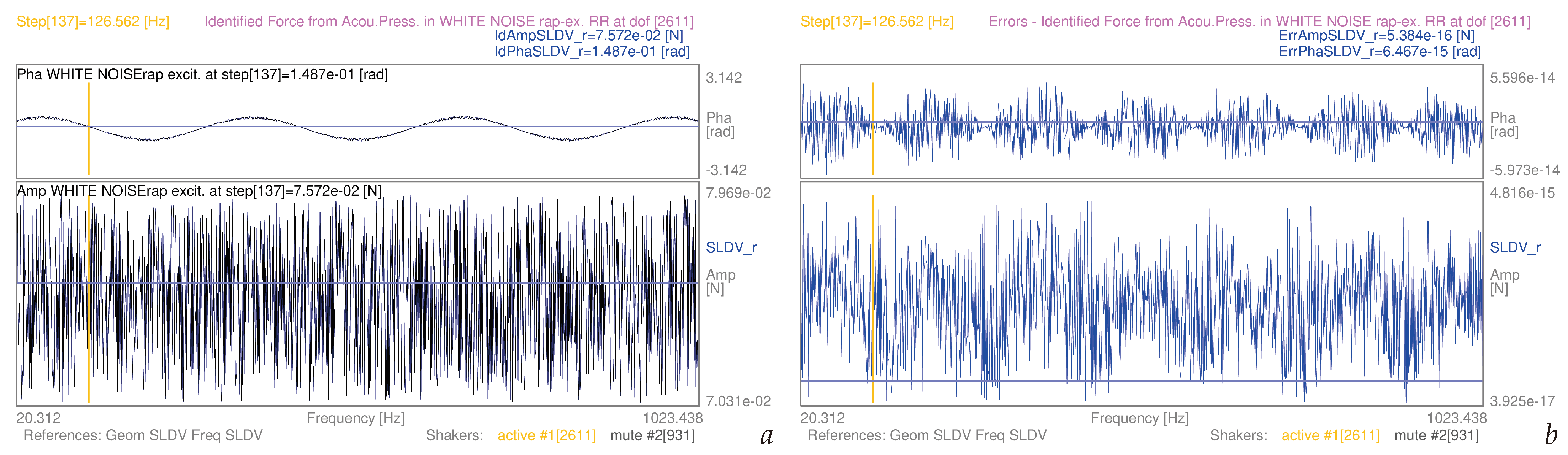
| 3.5 | (9) | whole mesh, white noise-rap | S1 | [20–1024] Hz | 12a | |
| 3.5 | (11) | whole mesh, white noise-rap | S1 | [20–1024] Hz | 12b | |
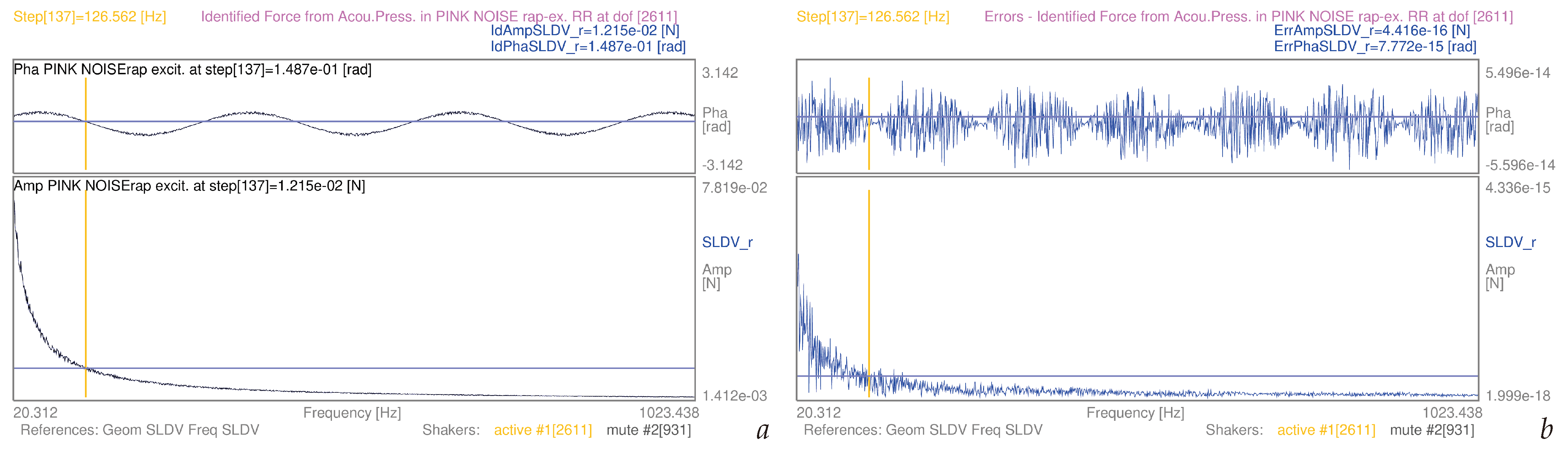
| 3.5 | (9) | whole mesh, pink noise-rap | S1 | [20–1024] Hz | 13a | |
| 3.5 | (11) | whole mesh, pink noise-rap | S1 | [20–1024] Hz | 13b | |
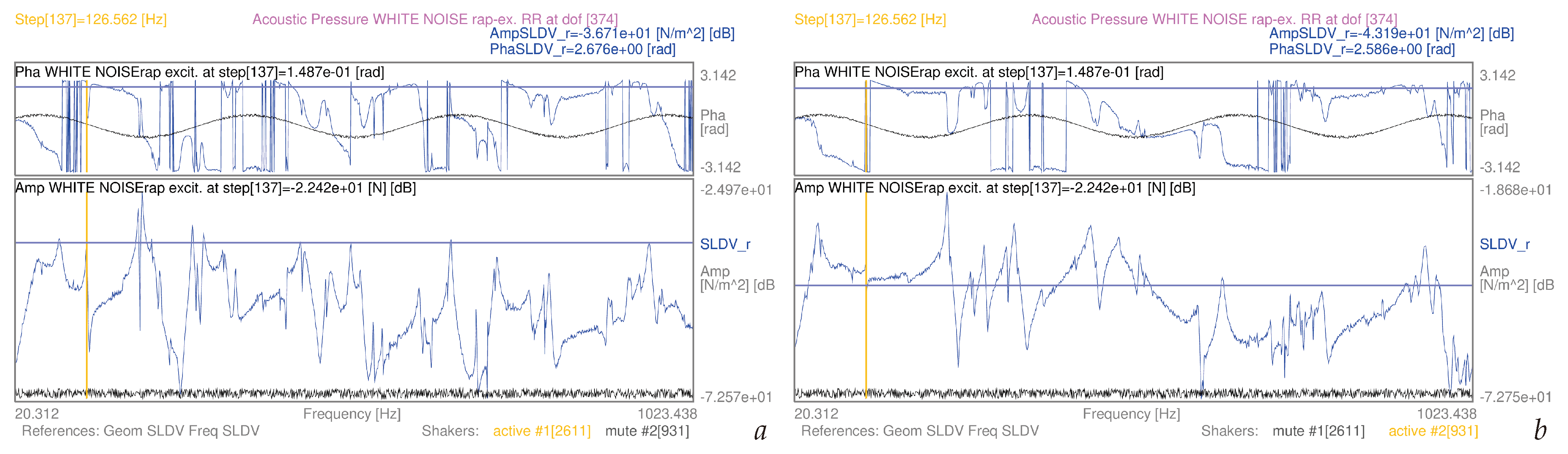
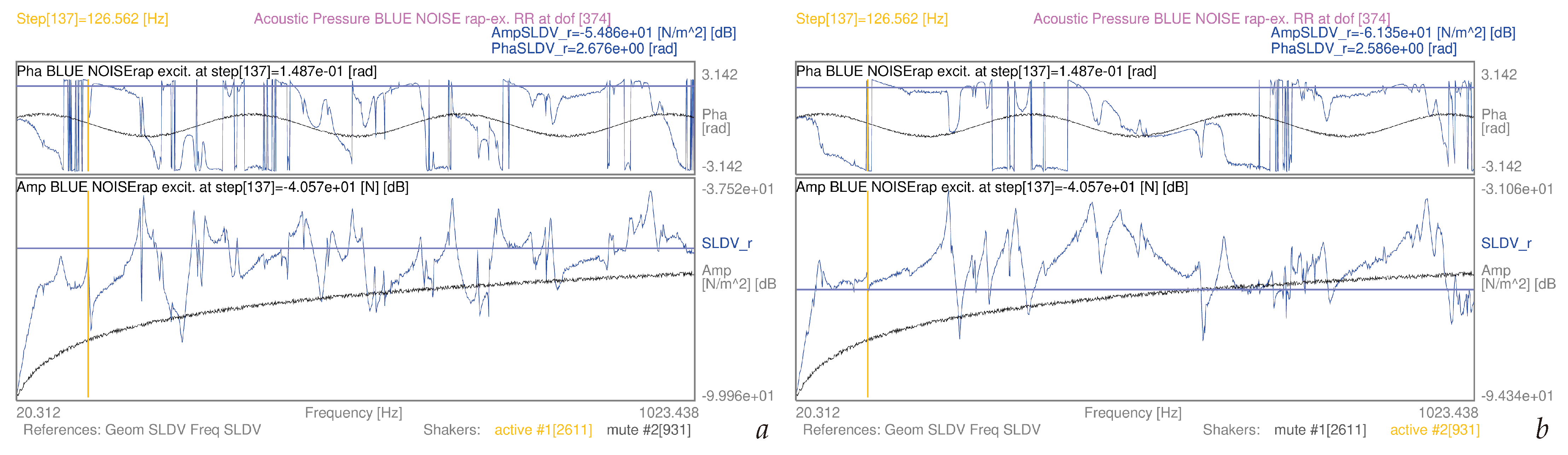
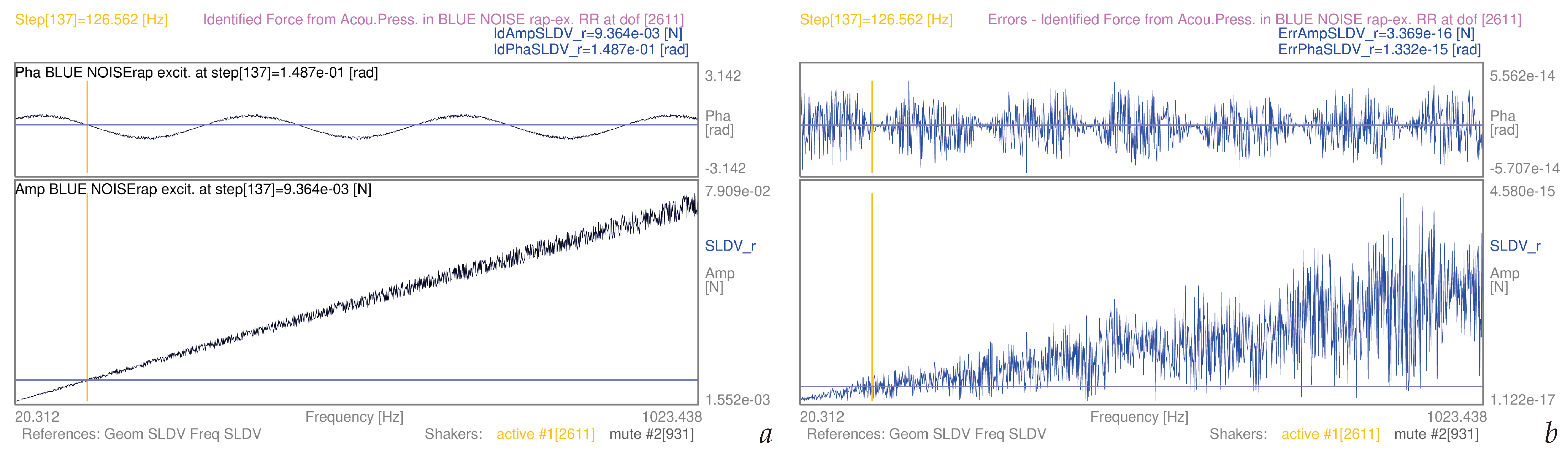
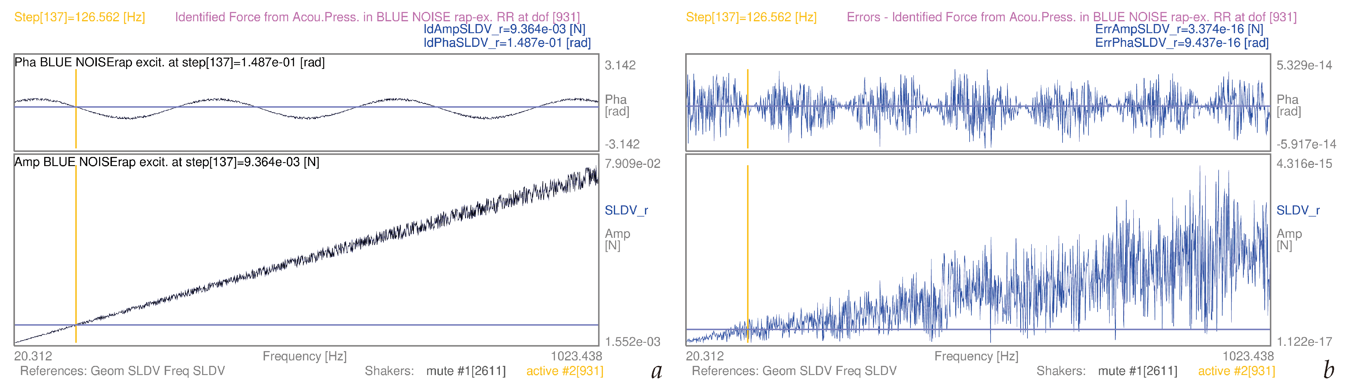
| 3.5 | (9) | whole mesh, blue noise-rap | S1 | [20–1024] Hz | 14a | |
| 3.5 | (11) | whole mesh, blue noise-rap | S1 | [20–1024] Hz | 14b | |
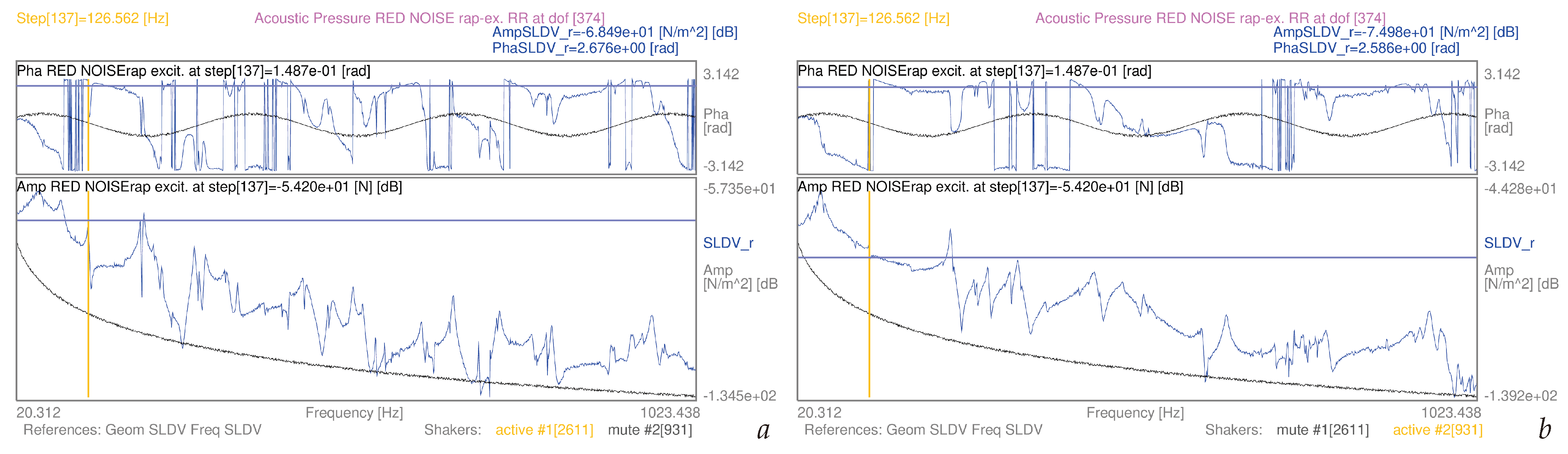
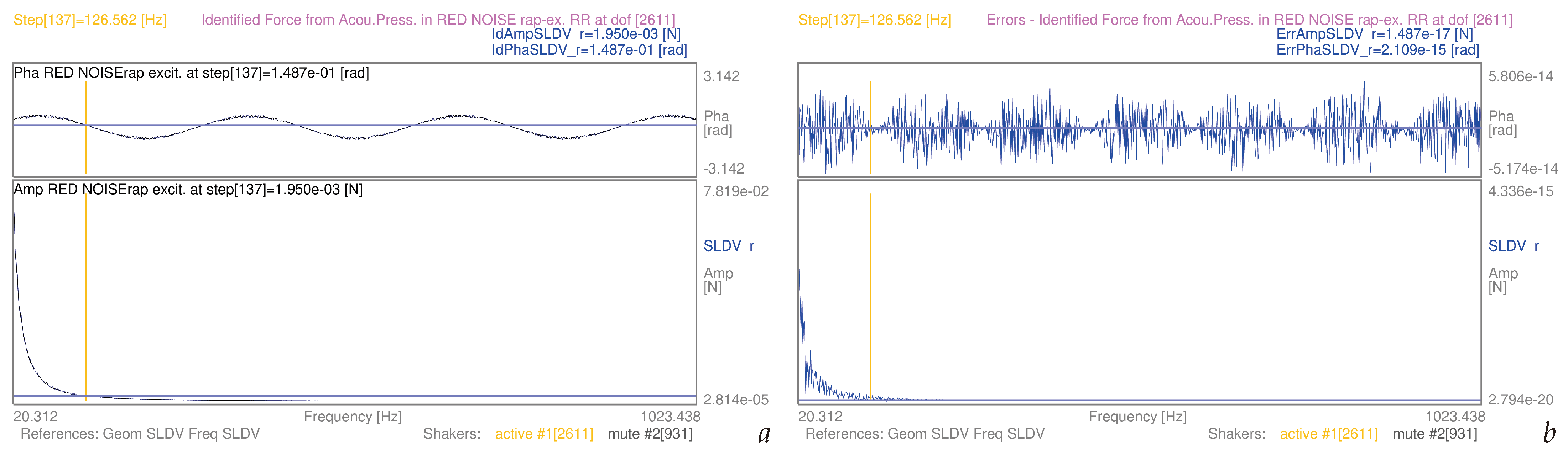
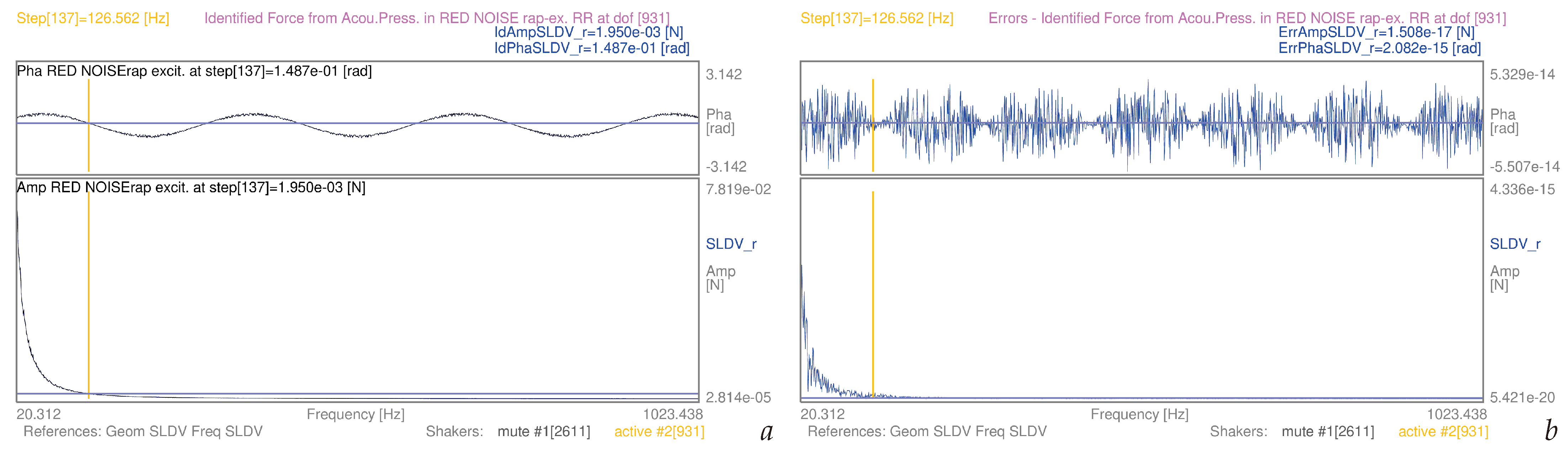
| 3.5 | (9) | whole mesh, red noise-rap | S1 | [20–1024] Hz | 15a | |
| 3.5 | (11) | whole mesh, red noise-rap | S1 | [20-1024] Hz | 15b | |
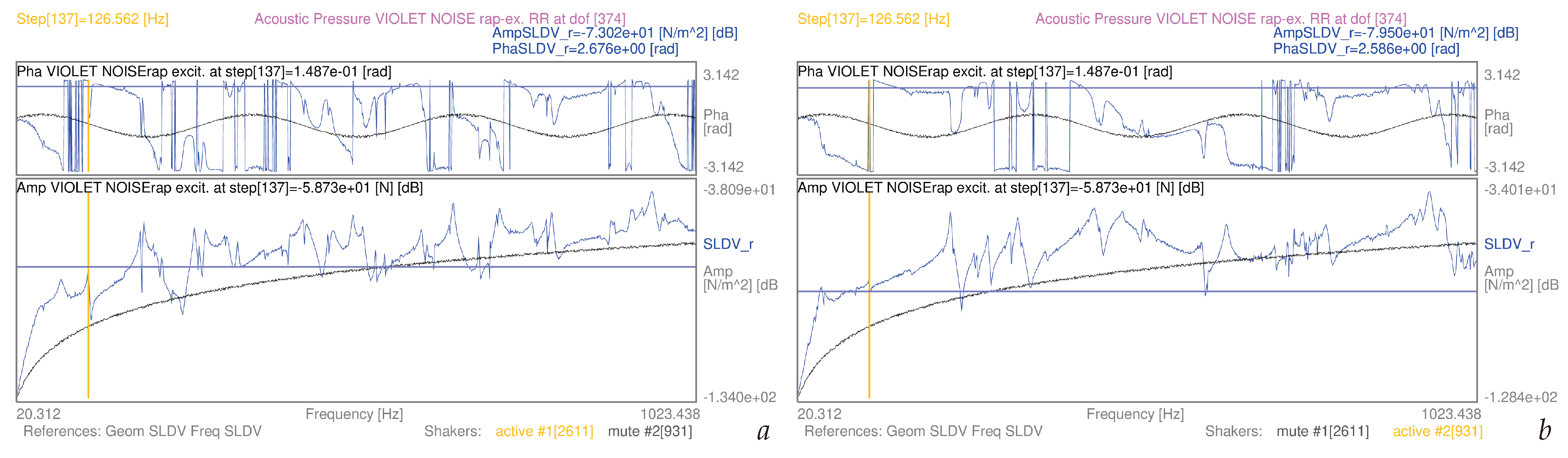
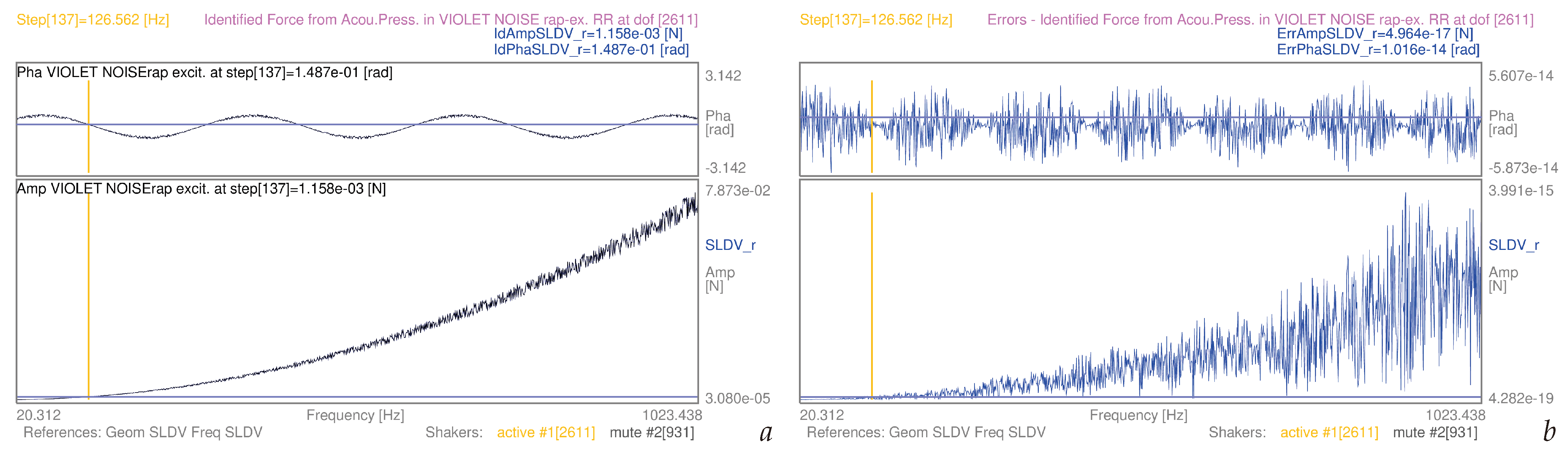
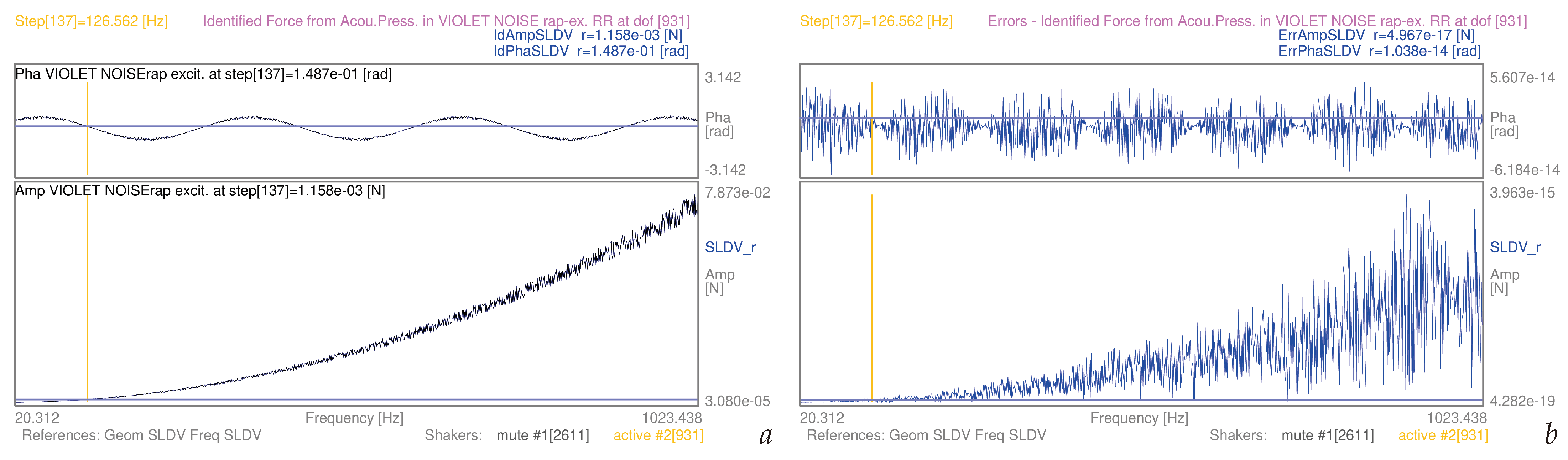
| 3.5 | (9) | whole mesh, violet noise-rap | S1 | [20–1024] Hz | 16a | |
| 3.5 | (11) | whole mesh, violet noise-rap | S1 | [20–1024] Hz | 16b | |
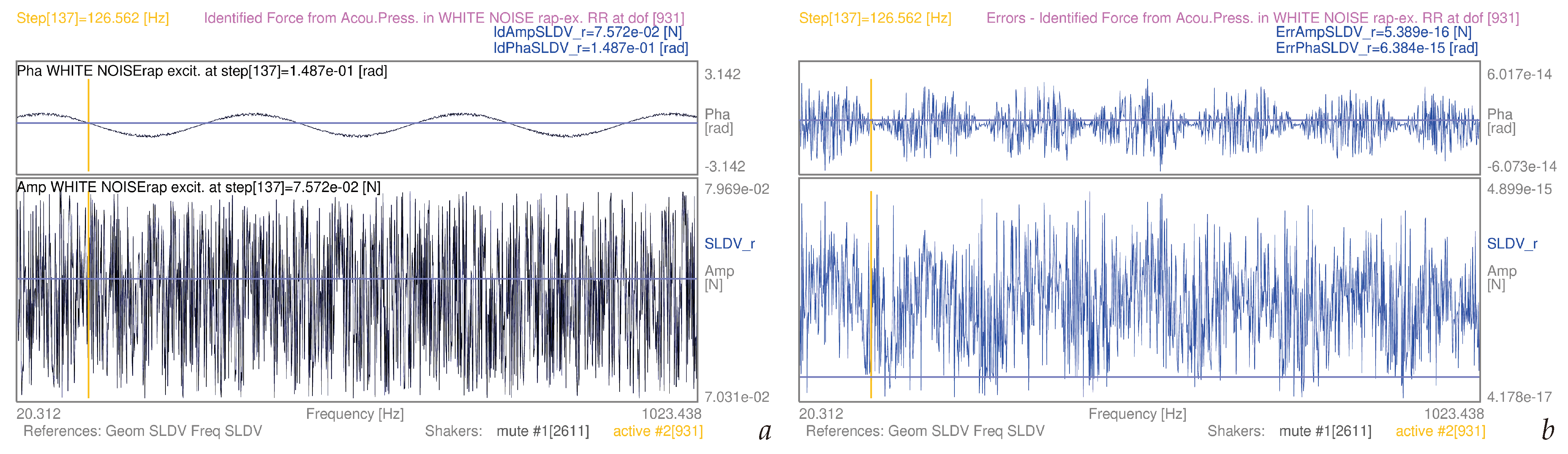
| 3.5 | (9) | whole mesh, white noise-rap | S2 | [20–1024] Hz | 17a | |
| 3.5 | (11) | whole mesh, white noise-rap | S2 | [20–1024] Hz | 17b | |
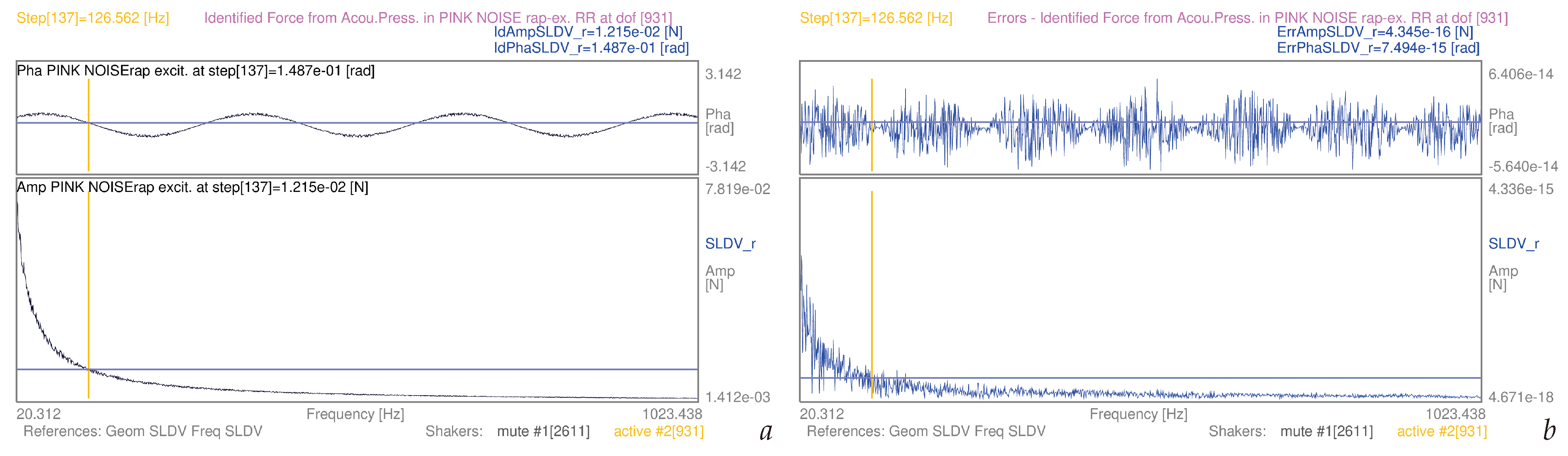
| 3.5 | (9) | whole mesh, pink noise-rap | S2 | [20–1024] Hz | 18a | |
| 3.5 | (11) | whole mesh, pink noise-rap | S2 | [20–1024] Hz | 18b | |
| 3.5 | (9) | whole mesh, blue noise-rap | S2 | [20–1024] Hz | 19a | |
| 3.5 | (11) | whole mesh, blue noise-rap | S2 | [20–1024] Hz | 19b | |
| 3.5 | (9) | whole mesh, red noise-rap | S2 | [20–1024] Hz | 20a | |
| 3.5 | (11) | whole mesh, red noise-rap | S2 | [20–1024] Hz | 20b | |
| 3.5 | (9) | whole mesh, violet noise-rap | S2 | [20–1024] Hz | 21a | |
| 3.5 | (11) | whole mesh, violet noise-rap | S2 | [20–1024] Hz | 21b |
3.1. Brief Notes on the Acoustic Domain Modelling

3.2. Vibro-Acoustic Transfer Matrices from Experiment-Based SLDV Mobilities
3.3. Acoustic Pressure Spectra from Experiment-Based SLDV Mobilities and Complex-Valued Forces

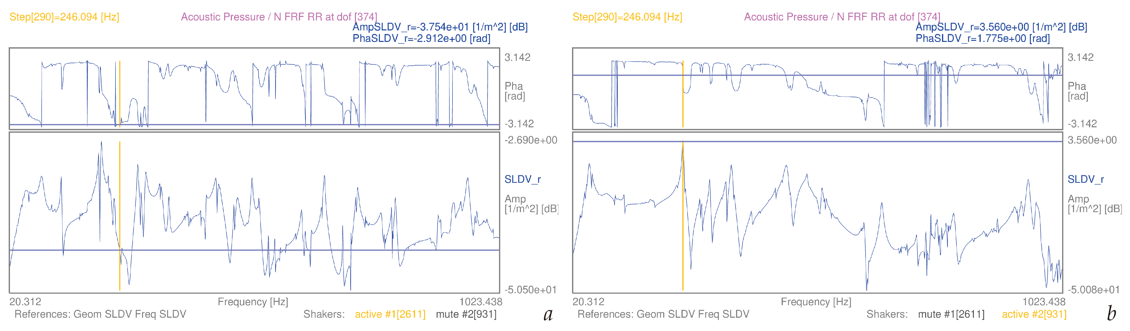
3.4. Airborne Acoustic-Vibrational FRFs from Experiment-Based SLDV Mobilities
3.5. Airborne Structural Force Evaluation as Induced by Known Pressure Fields
4. Discussion
| Noise Colour | Min Amp Err | Max Amp Err | Min Amp | Max Amp | Min Amp Err | Max Amp Err |
|---|---|---|---|---|---|---|
| + Shaker | [N] | [N] | [N] | [N] | / Min Amp | / Max Amp |
| white−rap S1 | 3.925e−17 | 4.816e−15 | 7.031e−02 | 7.969e−02 | 5.582e−16 | 6.043e−14 |
| white−rap S2 | 4.178e−17 | 4.899e−15 | 7.031e−02 | 7.969e−02 | 5.942e−16 | 6.148e−14 |
| pink−rap S1 | 1.999e−18 | 4.336e−15 | 1.412e−03 | 7.819e−02 | 1.416e−15 | 5.545e−14 |
| pink−rap S2 | 4.671e−18 | 4.336e−15 | 1.412e−03 | 7.819e−02 | 3.308e−15 | 5.545e−14 |
| blue−rap S1 | 1.122e−17 | 4.580e−15 | 1.552e−03 | 7.909e−02 | 7.229e−15 | 5.791e−14 |
| blue−rap S2 | 1.122e−17 | 4.316e−15 | 1.552e−03 | 7.909e−02 | 7.229e−15 | 5.457e−14 |
| red−rap S1 | 2.794e−20 | 4.336e−15 | 2.814e−05 | 7.819e−02 | 9.929e−16 | 5.545e−14 |
| red−rap S2 | 5.421e−20 | 4.336e−15 | 2.814e−05 | 7.819e−02 | 1.926e−15 | 5.545e−14 |
| violet−rap S1 | 4.282e−19 | 3.991e−15 | 3.080e−05 | 7.873e−02 | 1.390e−14 | 5.069e−14 |
| violet−rap S2 | 4.282e−19 | 3.963e−15 | 3.080e−05 | 7.873e−02 | 1.390e−14 | 5.034e−14 |
| Noise Colour | Min Pha Err | Max Pha Err | Min Pha | Max Pha | Min Pha Err | Max Pha Err |
|---|---|---|---|---|---|---|
| + Shaker | [rad] | [rad] | [rad] | [rad] | / Min Pha | / Max Pha |
| white−rap S1 | −5.973e−14 | 5.596e−14 | −1.901e−14 | 1.781e−14 | ||
| white−rap S2 | −6.073e−14 | 6.017e−14 | −1.933e−14 | 1.915e−14 | ||
| pink−rap S1 | −5.596e−14 | 5.496e−14 | −1.781e−14 | 1.749e−14 | ||
| pink−rap S2 | −5.640e−14 | 6.406e−14 | −1.795e−14 | 2.039e−14 | ||
| blue−rap S1 | −5.707e−14 | 5.562e−14 | −1.817e−14 | 1.770e−14 | ||
| blue−rap S2 | −5.917e−14 | 5.329e−14 | −1.883e−14 | 1.696e−14 | ||
| red−rap S1 | −5.174e−14 | 5.806e−14 | −1.647e−14 | 1.848e−14 | ||
| red−rap S2 | −5.507e−14 | 5.329e−14 | −1.753e−14 | 1.696e−14 | ||
| violet−rap S1 | −5.873e−14 | 5.607e−14 | −1.869e−14 | 1.785e−14 | ||
| violet−rap S2 | −6.184e−14 | 5.607e−14 | −1.968e−14 | 1.785e−14 |
5. Conclusions
Funding
Data Availability Statement
Acknowledgments
Conflicts of Interest
Abbreviations
| DIC | Digital image correlation |
| dof | Degree of freedom |
| EFFMA | Experimental full-field modal analysis |
| EMA | Experimental modal analysis |
| ESPI | Electronic speckle pattern interferometry |
| FRF | Frequency response function |
| NAH | Nearfield Acoustic Holography |
| NDT | Non-destructive testing |
| NVH | Noise and vibration harshness |
| ODS | Operative deflection shape |
| SLDV | Scanning laser Doppler vibrometer |
| Circular frequency dependency | |
| Velocity map | |
| Excitation force | |
| Mobility map | |
| Vibro-Acoustic FRFs | |
| Sound Pressure Fields mapping | |
| Pseudo-Inverse Vibro-Acoustic or Acoustic-Vibrational FRFs | |
| Identified Airborne Force | |
| Bold characters for array notation |
References
- Maynard, J.D.; Williams, E.G.; Lee, Y. Nearfield acoustic holography: I. Theory of generalized holography and the development of NAH. J. Acoust. Soc. Am. 1985, 78, 1395–1413. [Google Scholar] [CrossRef]
- Veronesi, W.A.; Maynard, J.D. Nearfield acoustic holography (NAH) II. Holographic reconstruction algorithms and computer implementation. J. Acoust. Soc. Am. 1987, 81, 1307–1322. [Google Scholar] [CrossRef]
- Williams, E.G. Fourier Acoustics: Sound Radiation and Nearfield Acoustical Holography; Elsevier Science: Amsterdam, The Netherlands, 1999. [Google Scholar] [CrossRef]
- Kirkup, S. Computational solution of the acoustic field surrounding a baffled panel by the Rayleigh integral method. Appl. Math. Model. 1994, 18, 403–407. [Google Scholar] [CrossRef]
- Gérard, F.; Tournour, M.; Masri, N.; Cremers, L.; Felice, M.; Selmane, A. Acoustic transfer vectors for numerical modeling of engine noise. Sound Vib. 2002, 36, 20–25. [Google Scholar]
- Fahy, F. Foundations of Engineering Acoustics; Academic Press: London, UK, 2003; pp. 1–443. [Google Scholar] [CrossRef]
- Desmet, W. Boundary Element Method in Acoustics. Technical Report, Katholieke Universiteit Leuven, Belgium, Mechanical Engineering Department, Noise & Vibration Research Group, 2004, for the ISAAC 15-Course on Numerical and Applied Acoustics.
- Kirkup, S.; Thompson, A. Computing the Acoustic Field of a Radiating Cavity by the Boundary Element-Rayleigh Integral Method (BERIM). In Proceedings of the World Congress on Engineering, WCE 2007, London, UK, 2–4 July 2007; Ao, S.I., Gelman, L., Hukins, D.W.L., Hunter, A., Korsunsky, A.M., Eds.; Lecture Notes in Engineering and Computer Science. Newswood Limited: Hong Kong, China, 2007; pp. 1401–1406. [Google Scholar]
- Arenas, J.P. Numerical computation of the sound radiation from a planar baffled vibrating surface. J. Comput. Acoust. 2008, 16, 321–341. [Google Scholar] [CrossRef]
- Arunkumar, M.; Pitchaimani, J.; Gangadharan, K.; Leninbabu, M. Vibro-acoustic response and sound transmission loss characteristics of truss core sandwich panel filled with foam. Aerosp. Sci. Technol. 2018, 78, 1–11. [Google Scholar] [CrossRef]
- Kirkup, S. The Boundary Element Method in Acoustics: A Survey. Appl. Sci. 2019, 9, 1642. [Google Scholar] [CrossRef]
- Lesoinne, M.; Sarkis, M.; Hetmaniuk, U.; Farhat, C. A linearized method for the frequency analysis of three-dimensional fluid/structure interaction problems in all flow regimes. Comput. Methods Appl. Mech. Eng. 2001, 190, 3121–3146, in Advances in Computational Methods for Fluid-Structure Interaction. [Google Scholar] [CrossRef]
- Sandberg, G.; Wernberg, P.A.; Davidsson, P. Fundamentals of Fluid-Structure Interaction. In Computational Aspects of Structural Acoustics and Vibration; Springer: Vienna, Austria, 2009; Volume 505, Chapter 2; pp. 23–101. [Google Scholar] [CrossRef]
- Ohayon, R.; Soize, C. Advanced computational dissipative structural acoustics and fluid-structure interaction in low- and medium-frequency domains. Reduced-order models and uncertainty quantification. Int. J. Aeronaut. Space Sci. 2012, 13, 127–153. [Google Scholar] [CrossRef]
- Vicente, W.; Picelli, R.; Pavanello, R.; Xie, Y. Topology optimization of frequency responses of fluid-structure interaction systems. Finite Elem. Anal. Des. 2015, 98, 1–13. [Google Scholar] [CrossRef]
- Zhou, Q.; Li, D.-f.; Da Ronch, A.; Chen, G.; Li, Y.-m. Computational fluid dynamics-based transonic flutter suppression with control delay. J. Fluids Struct. 2016, 66, 183–206. [Google Scholar] [CrossRef]
- Dowell, E.H.; Hall, K.C. Modeling of Fluid-Structure Interaction. Annu. Rev. Fluid Mech. 2001, 33, 445–490. [Google Scholar] [CrossRef]
- Kamakoti, R.; Shyy, W. Fluid-structure interaction for aeroelastic applications. Prog. Aerosp. Sci. 2004, 40, 535–558. [Google Scholar] [CrossRef]
- Werter, N.; De Breuker, R. A novel dynamic aeroelastic framework for aeroelastic tailoring and structural optimisation. Compos. Struct. 2016, 158, 369–386. [Google Scholar] [CrossRef]
- Li, D.; Zhou, Q.; Chen, G.; Li, Y. Structural dynamic reanalysis method for transonic aeroelastic analysis with global structural modifications. J. Fluids Struct. 2017, 74, 306–320. [Google Scholar] [CrossRef]
- Li, D.; Da Ronch, A.; Chen, G.; Li, Y. Aeroelastic global structural optimization using an efficient CFD-based reduced order model. Aerosp. Sci. Technol. 2019, 94, 105354. [Google Scholar] [CrossRef]
- Chen, Z.; Zhao, Y.; Huang, R. Parametric reduced-order modeling of unsteady aerodynamics for hypersonic vehicles. Aerosp. Sci. Technol. 2019, 87, 1–14. [Google Scholar] [CrossRef]
- Tian, W.; Gu, Y.; Liu, H.; Wang, X.; Yang, Z.; Li, Y.; Li, P. Nonlinear aeroservoelastic analysis of a supersonic aircraft with control fin free-play by component mode synthesis technique. J. Sound Vib. 2021, 493, 115835. [Google Scholar] [CrossRef]
- Wang, X.; Yang, Z.; Zhou, S.; Zhang, G. Complex damping influences on the oscillatory/static instability characteristics of heated panels in supersonic airflow. Mech. Syst. Signal Process. 2022, 165, 108369. [Google Scholar] [CrossRef]
- Patil, H.H.; Pitchaimani, J. Sound radiation characteristics of a beam under supersonic airflow and non-uniform temperature field. Aerosp. Sci. Technol. 2024, 147, 109001. [Google Scholar] [CrossRef]
- Heylen, W.; Lammens, S.; Sas, P. Modal Analysis Theory and Testing, 2nd ed.; Katholieke Universiteit Leuven: Leuven, Belgium, 1998; ISBN 90-73802-61-X. [Google Scholar]
- Ewins, D.J. Modal Testing-Theory, Practice and Application, 2nd ed.; Research Studies Press Ltd.: Baldock, UK, 2000; p. 400. ISBN 978-0-86380-218-8. [Google Scholar]
- Van der Auweraer, H.; Dierckx, B.; Haberstok, C.; Freymann, R.; Vanlanduit, S. Structural modelling of car panels using holographic modal analysis. In Proceedings of the 1999 Noise and Vibration Conference, Traverse City, MI, USA, 17 May 1999; Volume 3, pp. 1495–1506, SAE P-342. [Google Scholar] [CrossRef]
- Van der Auweraer, H.; Steinbichler, H.; Haberstok, C.; Freymann, R.; Storer, D. Integration of pulsed-laser ESPI with spatial domain modal analysis: Results from the SALOME project. In Proceedings of the 4th International Conference on Vibration Measurements by Laser Techniques: Advances and Applications, Ancona, Italy, 20–23 June 2000; SPIE: Bellingham, WA, USA, 2000; Volume 4072, pp. 313–322. [Google Scholar] [CrossRef]
- Van der Auweraer, H.; Steinbichler, H.; Haberstok, C.; Freymann, R.; Storer, D.; Linet, V. Industrial Applications of Pulsed-laser ESPI vibration analysis. In Proceedings of the XIX IMAC, SEM, Kissimmee, FL, USA, 5–8 February 2001; pp. 490–496. [Google Scholar]
- Van der Auweraer, H.; Steinbichler, H.; Vanlanduit, S.; Haberstok, C.; Freymann, R.; Storer, D.; Linet, V. Application of stroboscopic and pulsed-laser electronic speckle pattern interferometry (ESPI) to modal analysis problems. Meas. Sci. Technol. 2002, 13, 451–463. [Google Scholar] [CrossRef]
- Zanarini, A. Broad frequency band full field measurements for advanced applications: Point-wise comparisons between optical technologies. Mech. Syst. Signal Process. 2018, 98, 968–999. [Google Scholar] [CrossRef]
- Zanarini, A. Competing optical instruments for the estimation of Full Field FRFs. Measurement 2019, 140, 100–119. [Google Scholar] [CrossRef]
- Zanarini, A. Full field optical measurements in experimental modal analysis and model updating. J. Sound Vib. 2019, 442, 817–842. [Google Scholar] [CrossRef]
- Baqersad, J.; Poozesh, P.; Niezrecki, C.; Avitabile, P. Photogrammetry and optical methods in structural dynamics—A review. Mech. Syst. Signal Process. 2017, 86, 17–34, in SI: Full-field, non-contact vibration measurement methods: Comparisons and applications. [Google Scholar] [CrossRef]
- Wang, W.; Mottershead, J.E.; Ihle, A.; Siebert, T.; Schubach, H.R. Finite element model updating from full-field vibration measurement using digital image correlation. J. Sound Vib. 2011, 330, 1599–1620. [Google Scholar] [CrossRef]
- Wang, W.; Mottershead, J.; Siebert, T.; Pipino, A. Frequency response functions of shape features from full-field vibration measurements using digital image correlation. Mech. Syst. Signal Process. 2011, 28, 333–347. [Google Scholar] [CrossRef]
- LeBlanc, B.; Niezrecki, C.; Avitabile, P.; Sherwood, J.; Chen, J. Surface Stitching of a Wind Turbine Blade Using Digital Image Correlation. In Topics in Modal Analysis II, Proceedings of the 30th IMAC, A Conference on Structural Dynamics, SEM; Allemang, R., De Clerck, J., Niezrecki, C., Blough, J., Eds.; Springer: New York, NY, USA, 2012; Volume 6, pp. 277–284. [Google Scholar] [CrossRef]
- Ehrhardt, D.A.; Allen, M.S.; Yang, S.; Beberniss, T.J. Full-field linear and nonlinear measurements using Continuous-Scan Laser Doppler Vibrometry and high speed three-dimensional Digital Image Correlation. Mech. Syst. Signal Process. 2017, 86, 82–97. [Google Scholar] [CrossRef]
- Zanarini, A. On the making of precise comparisons with optical full field technologies in NVH. In Proceedings of the ISMA2020 Including USD2020—International Conference on Noise and Vibration Engineering, Leuven, Belgium, 7–9 September 2020; pp. 2293–2308, in Vol. Optical methods and computer vision for vibration engineering. [Google Scholar]
- Liu, W.; Ewins, D. The Importance Assessment of RDOF in FRF Coupling Analysis. In Proceedings of the IMAC 17th Conference, Kissimmee, FL, USA, 8–11 February 1999; Society for Experimental Mechanics (SEM): Bethel, CT, USA, 1999; pp. 1481–1487. [Google Scholar]
- Research Network. QUATTRO Brite-Euram Project no: BE 97-4184; Technical Report; European Commision Research Framework Programs: Brussels, Belgium, 1998. [Google Scholar]
- Friswell, M.; Mottershead, J.E. Finite Element Model Updating in Structural Dynamics; Solid Mechanics and Its Applications; Kuwler Academic Publishers & Springer Science+Business Media: Dordrecht, The Netherlands, 1995; p. 292. ISBN 978-0-7923-3431-6. [Google Scholar]
- Haeussler, M.; Klaassen, S.; Rixen, D. Experimental twelve degree of freedom rubber isolator models for use in substructuring assemblies. J. Sound Vib. 2020, 474, 115253. [Google Scholar] [CrossRef]
- Zanarini, A. Chasing the high-resolution mapping of rotational and strain FRFs as receptance processing from different full-field optical measuring technologies. Mech. Syst. Signal Process. 2022, 166, 108428. [Google Scholar] [CrossRef]
- Zanarini, A. Introducing the concept of defect tolerance by fatigue spectral methods based on full-field frequency response function testing and dynamic excitation signature. Int. J. Fatigue 2022, 165, 107184. [Google Scholar] [CrossRef]
- Zanarini, A. About the excitation dependency of risk tolerance mapping in dynamically loaded structures. In Proceedings of the ISMA2022 Including USD2022—International Conference on Noise and Vibration Engineering, Leuven, Belgium, 12–14 September 2022; pp. 3804–3818, in Vol. Structural Health Monitoring. [Google Scholar]
- Zanarini, A. Risk Tolerance Mapping in Dynamically Loaded Structures as Excitation Dependency by Means of Full-Field Receptances. In Proceedings of the IMAC XLI-International Modal Analysis Conference-Keeping IMAC Weird: Traditional and Non-Traditional Applications of Structural Dynamics, Austin, TX, USA, 13–16 February 2023; Chapter 9. Baqersad, J., Di Maio, D., Eds.; Springer Nature AG: Cham, Switzerland; SEM Society for Experimental Mechanics: Bethel, CT, USA, 2023; Computer Vision & Laser Vibrometry. Volume 6, pp. 43–56. [Google Scholar] [CrossRef]
- Zanarini, A. Exploiting DIC-based full-field receptances in mapping the defect acceptance for dynamically loaded components. Procedia Struct. Integr. 2024, 54C, 99–106, Proceedings of The 5th International Conference on Structural Integrity, 28 August–1 September 2023. [Google Scholar] [CrossRef]
- Zanarini, A. Mapping the defect acceptance for dynamically loaded components by exploiting DIC-based full-field receptances. Eng. Fail. Anal. 2024, 163, 108385. [Google Scholar] [CrossRef]
- Zanarini, A. On the approximation of sound radiation by means of experiment-based optical full-field receptances. In Proceedings of the ISMA2022 Including USD2022—International Conference on Noise and Vibration Engineering, Leuven, Belgium, 12–14 September 2022; pp. 2735–2749, in Vol. Optical Methods. [Google Scholar]
- Zanarini, A. Experiment-based Optical Full-field receptances in the Approximation of Sound Radiation from a Vibrating Plate. In Proceedings of the IMAC XLI-International Modal Analysis Conference-Keeping IMAC Weird: Traditional and Non-Traditional Applications of Structural Dynamics, Austin, TX, USA, 13–16 February 2023; Chapter 4. Baqersad, J., Di Maio, D., Eds.; Springer Nature AG: Cham, Switzerland; SEM Society for Experimental Mechanics: Bethel, CT, USA, 2023; Computer Vision & Laser Vibrometry. Volume 6, pp. 1–13. [Google Scholar] [CrossRef]
- Zanarini, A. On the influence of scattered errors over full-field receptances in the Rayleigh integral approximation of sound radiation from a vibrating plate. Acoustics 2023, 5, 948–986. [Google Scholar] [CrossRef]
- Zanarini, A. Assessing the retrieval procedure of complex-valued forces from airborne pressure fields by means of DIC-based full-field receptances in simplified pseudo-inverse vibro-acoustics. Aerosp. Sci. Technol. 2024, 157, 109757. [Google Scholar] [CrossRef]
- Zanarini, A. On the use of full-field receptances in inverse vibro-acoustics for airborne structural dynamics. Procedia Struct. Integr. 2024, 54C, 107–114, Proceedings of The 5th International Conference on Structural Integrity, 28 August–1 September 2023.. [Google Scholar] [CrossRef]
- Kreis, T. Handbook of Holographic Interferometry: Optical and Digital Methods; Wiley-VCH: Berlin, Germany, 2004. [Google Scholar] [CrossRef]
- Wind, J.; Wijnant, Y.; de Boer, A. Fast evaluation of the Rayleigh integral and applications to inverse acoustics. In Proceedings of the ICSV13, the Thirteenth International Congress on Sound and Vibration, Vienna, Austria, 2–6 July 2006; International Institute of Acoustics and Vibration (IIAV): Auburn, AL, USA, 2006; pp. 1–8. [Google Scholar]
- Michel Tournour, L.C.; Guisset, P.; Augusztinovicz, F.; Marki, F. Inverse Numerical Acoustics Based on Acoustic Transfer Vectors. In Proceedings of the 7th International Congress on Sound and Vibration—ICSV7, Garmisch-Partenkirchen, Germany, 4–7 July 2000; pp. 2069–2076. [Google Scholar]
- Citarella, R.; Federico, L.; Cicatiello, A. Modal acoustic transfer vector approach in a FEM-BEM vibro-acoustic analysis. Eng. Anal. Bound. Elem. 2007, 31, 248–258. [Google Scholar] [CrossRef]
- Guillaume, P.; Parloo, E.; De Sitter, G. Source identification from noisy response measurements using an iterative weighted pseudo-inverse approach. In Proceedings of the 2002 International Conference on Noise and Vibration Engineering, ISMA, Heverlee, Belgium, 16–18 September 2002; pp. 1817–1824. [Google Scholar]
- Vanlanduit, S.; Guillaume, P.; Cauberghe, B.; Parloo, E.; De Sitter, G.; Verboven, P. On-line identification of operational loads using exogenous inputs. J. Sound Vib. 2005, 285, 267–279. [Google Scholar] [CrossRef]
- Mas, P.; Sas, P. Acoustic Source Identification Based on Microphone Array Processing. Technical Report, Katholieke Universiteit Leuven, Belgium, Mechanical Engineering Department, Noise & Vibration Research Group, 2004, for the ISAAC 15-Course on Numerical and Applied Acoustics.
- Khoo, S.; Ismail, Z.; Kong, K.; Ong, Z.; Noroozi, S.; Chong, W.; Rahman, A. Impact force identification with pseudo-inverse method on a lightweight structure for under-determined, even-determined and over-determined cases. Int. J. Impact Eng. 2014, 63, 52–62. [Google Scholar] [CrossRef]
- Leclère, Q.; Pereira, A.; Bailly, C.; Antoni, J.; Picard, C. A unified formalism for acoustic imaging based on microphone array measurements. Int. J. Aeroacoustics 2017, 16, 431–456. [Google Scholar] [CrossRef]
- Chiariotti, P.; Martarelli, M.; Castellini, P. Acoustic beamforming for noise source localization—Reviews, methodology and applications. Mech. Syst. Signal Process. 2019, 120, 422–448. [Google Scholar] [CrossRef]
- Cumbo, R.; Tamarozzi, T.; Janssens, K.; Desmet, W. Kalman-based load identification and full-field estimation analysis on industrial test case. Mech. Syst. Signal Process. 2019, 117, 771–785. [Google Scholar] [CrossRef]
- Wikipedia.org. Speed of Sound. 2024. Available online: https://en.wikipedia.org/wiki/Speed_of_sound (accessed on 2 March 2024).
- Wikipedia.org. Density of Air. 2024. Available online: https://en.wikipedia.org/wiki/International_Standard_Atmosphere (accessed on 2 March 2024).
- Wikipedia.org. Machine Epsilon. 2024. Available online: https://en.wikipedia.org/wiki/Machine_epsilon (accessed on 18 April 2024).
| 1 | A. Zanarini is the scientific proposer & experienced researcher in the project TEFFMA—Towards Experimental Full Field Modal Analysis, financed by the EC—Marie Curie FP7-PEOPLE-IEF-2011 PIEF-GA-2011-298543 grant, 1 February 2013–31 July 2015. |
| 2 | In Proceedings of the ISMA2014 including USD2014—International Conference on Noise and Vibration Engineering, Leuven, Belgium, September 15–17, KU Leuven, 2014: see ‘On the estimation of frequency response functions, dynamic rotational degrees of freedom and strain maps from different full field optical techniques’ in Dynamic testing: methods and instrumentation; see ‘On the role of spatial resolution in advanced vibration measurements for operational modal analysis and model updating’ in Operational modal analysis. |
| 3 | In Proceedings of the ICoEV2015 International Conference on Engineering Vibration, Ljubljana, Slovenia, September 7–10, Univ. Ljubljana & IFToMM, 2015, symposium Full Field Measurements for Advanced Structural Dynamics, see: ‘Model updating from full field optical experimental datasets’; ‘Comparative studies on full field FRFs estimation from competing optical instruments’; ‘Accurate FRFs estimation of derivative quantities from different full field measuring technologies’; ‘Full field experimental modelling in spectral approaches to fatigue predictions’. |
| 4 | |
| 5 | Specifically, a risk index was firstly introduced in On the defect tolerance by fatigue spectral methods based on full-field dynamic testing to locate the areas mostly exposed to failure in a part subjected to dynamic load, while in On the exploitation of multiple 3D full-field pulsed ESPI measurements in damage location assessment a damaged composite panel was tested in the same perspective. Recently, in [46], ESPI-based risk map variability was addressed by real-valued amplitude excitation signatures; the effect of the energy-injection location was investigated in [47]; both aspects were gathered in [48]. Although reduced—by interpolation in both spatial and frequency domains—to the more moderate resolutions of the SLDV references in the TEFFMA project, DIC-based full-field receptances were used instead in [49] for the risk index mapping. Instead, in [50] the raw datasets from DIC—with no numerical residuals due to the topology transforms and interpolations—boosted the risk index analyses; furthermore, the latter used complex-valued coloured noises for force signals, with potential randomness in the complex amplitude and phase. |
| 6 | Specifically, in [51,52] the ESPI technique was used to explore the viability of the direct vibro-acoustic modelling, while in [53] the effect of errors on vibro-acoustics from SLDV-based mobilities was investigated; in [54] raw DIC-based were used without transforms’ errors for pseudo-inverse vibro-acoustics. |
| 7 | It was held at Dantec Ettemeyer GmbH, Ulm, Germany. In particular, for the main achievements, see: ‘Full field ESPI measurements on a plate: challenging experimental modal analysis’, in: Proceedings of the XXV IMAC, Orlando (FL) USA, Feb 19–22, SEM, 2007; ‘Fatigue life assessment by means of full field ESPI vibration measurements’ in: P. Sas (Ed.), Proceedings of the ISMA2008 Conference, September 15–17, Leuven (Belgium); ‘Full field ESPI vibration measurements to predict fatigue behaviour’, in: Proceedings of the IMECE2008 ASME International Mechanical Engineering Congress and Exposition, October 31–November 6, Boston (MA), USA. |
| 8 | Working on the information obtainable in [67,68], one can see how, at sea level, varies in the range of [315.77–351.88] m/s and in the range [1.4224–1.1455] kg/m3 as the temperature rises from −25 °C to +35 °C. Furthermore, with the altitude flattens to about 295–300 m/s, while is more variable, in rising from the Troposphere (0–11 km) into the Tropopause (11–20 km), having a strongly variable range [1.225 (sea level, 15 °C)–0.3639 (11 km, −56.5 °C)–0.088 (20 km, −56.5 °C)] kg/m3. |
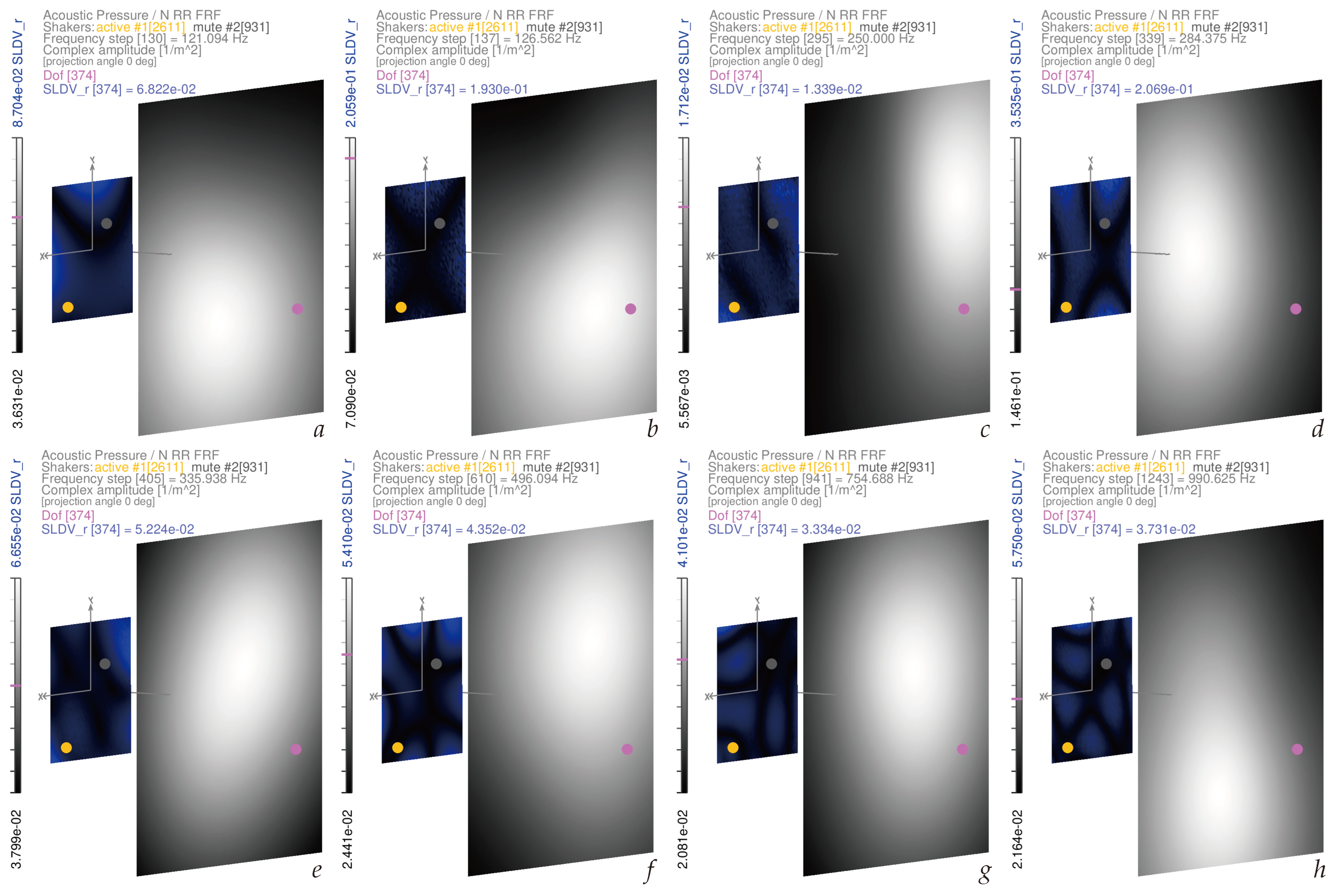
| 9 | In particular, when the vibrating surface is at nearfield distance, it can reveal the proximity to specific nodal lines of the structural ODSs, especially at lower frequencies. The motion of the structural ODS in the extreme corners also seem to have some relevance here onto the far distance blending of the vibro-acoustic transfer matrix. Instead, as was shown in [53], at closer distances the structural ODS projects into the vibro-acoustic transfer matrix mesh with a much clearer reproduction of nodal lines’ pattern. This was also manifest in [54], where the complex amplitude on the acoustic mesh mixes in a smoother field those components, coming from a more articulated pattern in the structural ODS. |
| 10 | The custom C-language/OpenMP computational engine, written by the author, exploits the 64-bit machine computational precision (see [69]) for double floating numbers, or machine epsilon of . |
| 11 | The dataset used—1285 frequency lines, 2601 acoustic dofs, 2907 structural dofs—for each simulation needed the peak allocation of 145.7 GB of RAM, accessed simultaneously by 24 logical threads in parallel OpenMP-based computing in the custom C-language code, gcc 7.5.0 target:x86_64-suse-linux in OpenSUSE® Linux environment with kernel 6.4, and on a workstation with 192 GB of RAM, 12 physical cores in dual hexacore Intel® Xeon® X5690 CPUs running at 3.46–3.73 GHz. After the data loading, the vibro-acoustic transfer matrix was computed in around 35 s, while the successive evaluations of the acoustic-vibrational FRF , of the airborne force and relative errors took around 21 s. |
| Section | Equation | Quantity | Structural | Acoustic | Frequency | Figure |
|---|---|---|---|---|---|---|
| Excitation | Domain | Domain | ||||
| 3.2 | (7) | S1, – | single dof [374] | [20–1024] Hz | 3a | |
| 3.2 | (7) | S2, – | single dof [374] | [20–1024] Hz | 3b | |
| 3.2 | (7) | S1, – | whole mesh | 121.1 Hz | 4a | |
| 3.2 | (7) | S1, – | whole mesh | 127.5 Hz | 4b | |
| 3.2 | (7) | S1, – | whole mesh | 250.0 Hz | 4c | |
| 3.2 | (7) | S1, – | whole mesh | 284.4 Hz | 4d | |
| 3.2 | (7) | S1, – | whole mesh | 335.9 Hz | 4e | |
| 3.2 | (7) | S1, – | whole mesh | 496.1 Hz | 4f | |
| 3.2 | (7) | S1, – | whole mesh | 754.7 Hz | 4g | |
| 3.2 | (7) | S1, – | whole mesh | 990.6 Hz | 4h | |
| 3.2 | (7) | S2, – | whole mesh | 121.1 Hz | 5a | |
| 3.2 | (7) | S2, – | whole mesh | 127.5 Hz | 5b | |
| 3.2 | (7) | S2, – | whole mesh | 250.0 Hz | 5c | |
| 3.2 | (7) | S2, – | whole mesh | 284.4 Hz | 5d | |
| 3.2 | (7) | S2, – | whole mesh | 335.9 Hz | 5e | |
| 3.2 | (7) | S2, – | whole mesh | 496.1 Hz | 5f | |
| 3.2 | (7) | S2, – | whole mesh | 754.7 Hz | 5g | |
| 3.2 | (7) | S2, – | whole mesh | 990.6 Hz | 5h |
| Section | Equation | Quantity | Structural | Acoustic | Frequency | Figure |
|---|---|---|---|---|---|---|
| Excitation | Domain | Domain | ||||
| 3.3 | (8) | S1, white noise-rap | single dof [374] | [20–1024] Hz | 6a | |
| 3.3 | (8) | S2, white noise-rap | single dof [374] | [20–1024] Hz | 6b | |
| 3.3 | (8) | S1, pink noise-rap | single dof [374] | [20–1024] Hz | 7a | |
| 3.3 | (8) | S2, pink noise-rap | single dof [374] | [20–1024] Hz | 7b | |
| 3.3 | (8) | S1, blue noise-rap | single dof [374] | [20–1024] Hz | 8a | |
| 3.3 | (8) | S2, blue noise-rap | single dof [374] | [20–1024] Hz | 8b | |
| 3.3 | (8) | S1, red noise-rap | single dof [374] | [20–1024] Hz | 9a | |
| 3.3 | (8) | S2, red noise-rap | single dof [374] | [20–1024] Hz | 9b | |
| 3.3 | (8) | S1, violet noise-rap | single dof [374] | [20–1024] Hz | 10a | |
| 3.3 | (8) | S2, violet noise-rap | single dof [374] | [20–1024] Hz | 10b |
Disclaimer/Publisher’s Note: The statements, opinions and data contained in all publications are solely those of the individual author(s) and contributor(s) and not of MDPI and/or the editor(s). MDPI and/or the editor(s) disclaim responsibility for any injury to people or property resulting from any ideas, methods, instructions or products referred to in the content. |
© 2025 by the author. Licensee MDPI, Basel, Switzerland. This article is an open access article distributed under the terms and conditions of the Creative Commons Attribution (CC BY) license (https://creativecommons.org/licenses/by/4.0/).
Share and Cite
Zanarini, A. Attempts at Pseudo-Inverse Vibro-Acoustics by Means of SLDV-Based Full-Field Mobilities. Machines 2025, 13, 324. https://doi.org/10.3390/machines13040324
Zanarini A. Attempts at Pseudo-Inverse Vibro-Acoustics by Means of SLDV-Based Full-Field Mobilities. Machines. 2025; 13(4):324. https://doi.org/10.3390/machines13040324
Chicago/Turabian StyleZanarini, Alessandro. 2025. "Attempts at Pseudo-Inverse Vibro-Acoustics by Means of SLDV-Based Full-Field Mobilities" Machines 13, no. 4: 324. https://doi.org/10.3390/machines13040324
APA StyleZanarini, A. (2025). Attempts at Pseudo-Inverse Vibro-Acoustics by Means of SLDV-Based Full-Field Mobilities. Machines, 13(4), 324. https://doi.org/10.3390/machines13040324