Abstract
Operational safety and fuel efficiency are critical, yet often conflicting, objectives in modern civil get engine designs. Optimal efficiency operating conditions are typically close to unsafe regions, such as compressor stalls, which can cause severe engine damage. Consequently, engines are generally operated below peak efficiency to maintain a sufficient stall margin. Reducing this margin through active control requires stall precursor detection and mitigation mechanisms. While several algorithms have shown promising results in predicting modal stalls, predicting spike stalls remains a challenge due to their rapid onset, leaving little time for corrective actions. This study addresses this gap by proposing a method to identify spike stall precursors based on the changing dynamics within a compressor blade passage. An autoregressive time series model is utilized to capture these dynamics and its changes are related to the flow condition within the blade passage. The autoregressive model is adaptively extracted from measured pressure data from a one-stage axial compressor test stand. The corresponding eigenvalues of the model are monitored by utilizing an outlier detection mechanism that uses pressure reading statistics. Outliers are proposed to be associated with spike stall precursors. The model order, which defines the number of relevant eigenvalues, is determined using three information criteria: the Akaike Information Criterion (AIC), the Bayesian Information Criterion (BIC), and the Conditional Model Estimator (CME). For prediction, an outlier detection algorithm based on the Generalized Extreme Studentized Deviate (GESD) Test is introduced. The proposed method is experimentally validated on a single-stage low-speed axial compressor. Results demonstrate consistent stall precursor detection, with future application for timely control interventions to prevent spike stall inception.
1. Introduction
Compressor stalls are a critical issue in the operation of axial and centrifugal compressors in jet engines and gas turbines. This phenomenon, characterized by a disruption of the smooth airflow through the compressor blades, can lead to severe performance degradation and even failure of the engine. Near the stability limit, uneven flow can cause local flow separation, creating a blockage that alters airflow through adjacent blade passages. This shifting of stalled and unstalled regions propagates around the compressor, forming a rotating stall, which moves at 20–80% of rotor speed [1].
Compressor stalls are typically classified into two main types: spike stalls and modal stalls. Each type has distinct characteristics and implications for engine performance. Spike stalls are abrupt and can occur with minimal warning, making them particularly hazardous. In contrast, modal stalls develop gradually with wave-like instabilities, offering a potential window for detection and mitigation. The evolution and effects of these stalls have been explored extensively in the literature [2]. Since the phenomenon was first documented in the 1940s [3], research interest in rotating stall behavior and control strategies has fluctuated. Given the severe consequences of stall events, a considerable portion of the research effort has focused on predicting and preventing them. Early detection is essential as it enables timely intervention strategies to mitigate or entirely avoid compressor stalls. Various algorithms have been proposed to identify indicators of stall inception before it fully manifests.
Detecting the onset of compressor stalls, particularly spike stalls, presents significant challenges. One of the primary indicators of stall initiation is the instability of fluid pressure across the compressor blade passages. However, this instability emerges suddenly and unpredictably, making early detection difficult. Despite significant advances in rotating stall research since World War II, the prediction of compressor stall behavior has not seen equivalent progress [4]. Most advancements have been made in the study of modal stalls, leaving spike stall prediction relatively underdeveloped.
In a study in 1991, Inoue et al. [5] examined the statistical patterns of pressure fluctuations along the casing wall to identify precursors to rotating stalls. They observed highly erratic pressure behavior near the leading edge as stall inception approached. By evaluating the cross-correlation of pressure fluctuations at different measurement points, they demonstrated the potential for stall prediction. Given the gradual degradation of periodicity in pressure fluctuations and the use of statistical methodologies, it is likely that their study focused on modal stall. Further research in 1995 by Tryfonidis [6] analyzed nine compressors using the traveling wave energy method as a stall warning mechanism. Their results indicated that modal stall onset could be predicted 100–200 rotor revolutions in advance. However, this approach was found to be ineffective in predicting spike stalls. Similarly, Day et al. [7] explored the role of stage matching in stall prediction, employing spatial Fourier decomposition and traveling wave energy analysis. Their findings reinforced the effectiveness of these techniques for modal stall detection, with a predictive window of 50 to 100 revolutions before stall onset. However, these methods proved inadequate for spike stall prediction, as the warning period was significantly shorter. More recently, Heinlein et al. (2017) [8] applied Grubb’s test to detect anomalies as indicators of stall precursors. Their statistical analysis approach allowed for stall detection 16.5 revolutions before occurrence. However, the practical application of Grubb’s test is constrained by the need to predetermine the number of outliers, which is difficult as the threshold for stall-triggering anomalies is not fixed. In 2019, Li and Zhang [9] utilized fast wavelet analysis for stall prediction. Their study demonstrated that low-frequency reconstruction might enhance spike stall prediction, though they did not quantify their findings. Aung and Schoen (2019) [10] evaluated multiple statistical approaches—including autocorrelation, special entropy, and autoregression—to determine the most effective method for spike stall prediction. Their study identified autoregression as the most reliable approach, enabling stall prediction up to 16 rotor revolutions before onset. While numerous methodologies have been proposed for detecting stall precursors, many fail to provide sufficient warning time for effective intervention. The unpredictable nature of pressure instabilities and the rapid development of spike stalls underscore the need for more precise and reliable prediction techniques.
In this paper, the onset of spike stall is attempted to be predicted at the earliest time possible using an autoregressive (AR) model. AR models use the past data to predict the next state of the system dynamics, assuming the system is a Markov process, i.e., the present event is dependent only on the past event. The hypothesis of the proposed research is that when a stall is initiated, something in the dynamics of the system must have changed (though not visibly) that could indicate the onset of a stall event. If the pressure values are observed, they do not show any indication that a stall is going to occur. In this work, the eigenvalues of the extracted AR model capturing the dynamics of the fluid flow within the blade passage are used as an indicator of the onset of stall. If the prediction horizon is sufficient using the proposed method, control techniques could be applied in time to prevent the stalling event. This allows the jet engine to operate closer to the point of maximum efficiency without stalling. While working on autoregressive models, the order of the model needs to be determined. In this work, the information criteria, such as Akaike Information Criteria (AIC), Bayesian Information Criteria (BIC), and Conditional Model Estimator (CME), will be studied to determine the order of autoregressive models.
2. Theory
2.1. Autoregressive Model
One of the important applications of time series analysis is forecasting future values from the present and past values [11]. An autoregressive model is a stochastic dynamic mathematical model in which the current value is the sum of a linear combination of previous values. The AR model of order p can be defined mathematically as
where refers to the current value in the time series; refer to the coefficients of the model. The coefficients are the weights applied to the past values of the time series; refer to the past values of the time series; is the order of the AR model, determining how many data points from the past are utilized to predict the future; is the residual or the error term, i.e., the difference between the actual value and the predicted value.
In matrix form, the above equation can be written as
where is the output vector and defined as ; is the information matrix and defined as ; is the parameter vector and defined as
There are several algorithms that can solve the estimation problem. For the present research, computational speed and computational load are not considered, and for simplicity, a standard least-square approach is utilized. This method allows for future implementation when converting it into a recursive form, hence avoiding matrix inversion. The least-square estimate of the parameter vector is . The roots of the parameter vector are the eigenvalues, which describe the dynamics of the system.
2.2. Information Criteria
In AR modeling, determining the appropriate model order is crucial. Selecting the correct order is essential because if the chosen order is lower than the true order, the estimated parameters will be inconsistent. Conversely, if the order is higher than the true order, it can result in overfitting the system it is modeling [12]. Various statistical methods exist for determining the AR model order, and in this study, information criteria are employed for this purpose. Information criteria help select the best mathematical model from a set of candidate models with different numbers of unknown parameters.
Among the commonly used criteria, Akaike Information Criteria (AIC), Bayesian Information Criteria (BIC), and Conditional Model Estimator (CME) are considered in this work. AIC, developed by the Japanese statistician Hirotugu Akaike (1974) [13], selects models by balancing goodness of fit with complexity and is defined as
where is the number of parameters in the model, n is the sample size, and is the residual sum of squares, given by
where is the vector of actual data and is the output vector of the estimated value obtained from the AR model.
The model having the lowest value of AIC is considered the best model. Some of the examples of application of AIC, which is most studied in the literature to determine the order of an AR model, can be found in [14,15,16].
Similarly, BIC, which also balances fit and complexity but includes a stronger penalty for model size, is given by
In addition to AIC and BIC, CME, proposed by Steve Kay (2001) [17], is also employed. Unlike AIC and BIC, CME does not require prior knowledge of the model parameters and is defined as
where the estimate of ;
; is the gamma function.
A comparison of these methods can be found in [18]. This work utilizes the best result among AIC, BIC, and CME to determine the final model order.
The above-mentioned criteria tend to select a single model from the candidates of models. The authors in [19] argue that, while selecting one model, the single-model approach misses the potentially significant information carried by other models. They explain a method of using multiple models together, called multiple model identification, rather than using a single model. Then, the problem is transformed into an estimation problem where the probability of each model being correct is calculated to improve predictions. This method, Bayesian Model Averaging (BMA), combines the predictions from all models, weighting each model by its probability of being correct. The model probabilities are calculated using penalty terms from model selection criteria like AIC, BIC, CME, etc., which are mathematically defined as
where ‘l’ represents the corresponding value of AIC, BIC, and CME, respectively. The model with the highest probability of being correct is chosen as the order of the AR model in this work. A similar application of modal probability can be found in [18].
2.3. Generalized Extreme Studentized Deviate (GESD) Test
The GESD test is a statistical method used for outlier detection in univariate data and when the data set is large. Since the datasets used in this research have a single variable, i.e., pressure, and the size of the data is large, GESD becomes suitable for outlier detection. The GESD test is also useful when the number of outliers in the dataset is unknown since it requires only the maximum number of outliers to be detected in the sample [20]. The GESD test is performed by taking the following steps:
- The maximum number of outliers to be detected is defined.
- The significance level of the test, α, is defined. In this study, 0.05 is selected as the significance level.
- The mean, , and standard deviation, , of the sample is calculated
- Test statistic, , is calculated.
- The critical values, , are calculated, where is the adjusted significance level; is the sample size; is the degree of freedom, and is the critical value of the t-distribution with degrees of freedom.
- The sample size is reduced by removing the maximum value of R, i.e., the maximum outlier.
- Steps 3 through 5 are repeated till the outlier is detected.
- The number of times the maximum value of R is removed gives the maximum number of outliers present in the data sample.
In this study, the GESD test, along with the expanding window algorithm, is used to find the number of outliers.
3. Experimental Setup
3.1. Compressor Geometry
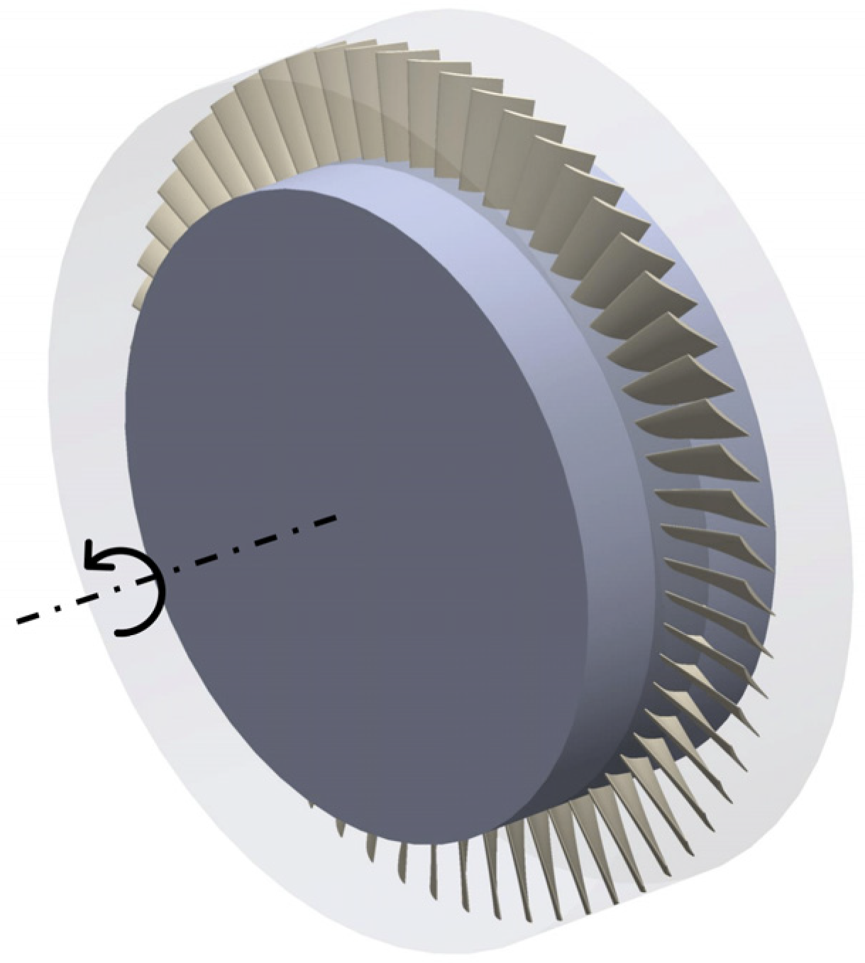
The experimental research is conducted on a low-speed single-rotor axial flow compressor. The compressor is driven by a direct current motor with a power rating of 22.5 kW, and its design speed is 2400 rpm. An overview of the rotor blade assembly is shown in Figure 1, which provides a 3D visualization of the rotor configuration used in the experiment. This figure illustrates the spatial arrangement of the 60 rotor blades and the direction of rotation, offering a clear view of the physical geometry relevant to the test setup.
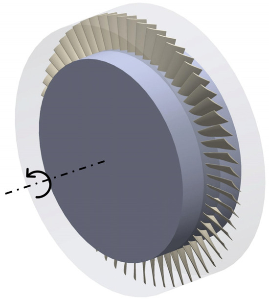
Figure 1.
Three-dimensional view of the single-stage axial compressor rotor blade assembly used in the experiment. The figure illustrates the blade arrangement and rotation direction of the rotor.
A linear module is installed at the outlet throttling valve base to achieve gradual and uniform throttling of the valve, thus allowing for precise control of the compressor flow rate. The specific parameters of the compressor are provided in Table 1.

Table 1.
Main parameters of the test rig.
The focus of this study is on utilizing pressure data obtained from the compressor to identify spike stall precursors through a data-driven modeling approach. The geometric and operational parameters listed in Table 1 represent the key details of the test rig as recorded during the experimental campaign. However, it is important to note that this work does not aim to analyze or optimize the aerodynamic design of the compressor. Parameters such as spanwise variations in inlet and outlet blade angles or incidence angles were not part of the experimental measurements, as they fell outside the scope of this study. Our primary objective is to evaluate the effectiveness of the proposed stall precursor prediction method based on the available pressure measurements.
3.2. Compressor Characteristic Line
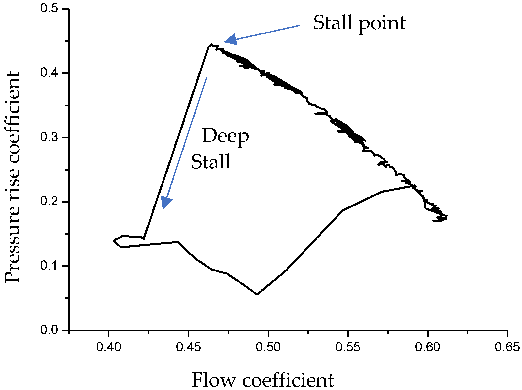
Figure 2 depicts the characteristics of the single-stage axial compressor used for the experimentation. The graph is generated by running the compressor into a deep stall at the design speed of 2400 rpm. A stall occurs around a flow coefficient of 0.47.
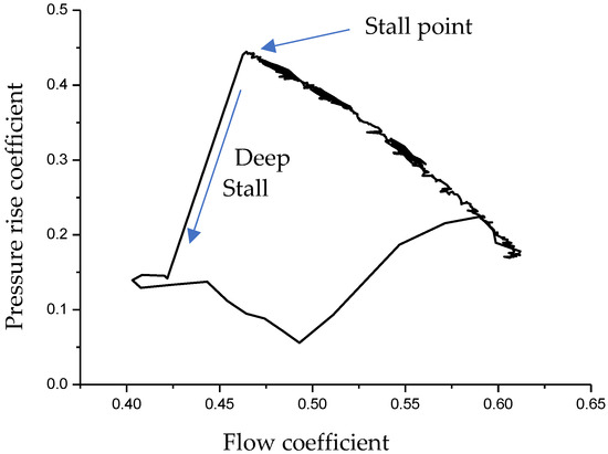
Figure 2.
Characteristic curve of a single-stage axial compressor depicting the flow coefficient and its resulting pressure changes. The characteristics are found by reducing the flow coefficient during experimentation using the throttle. Spike stall occurs at a flow coefficient of approximately 0.47.
4. Methodology
4.1. Data Collection
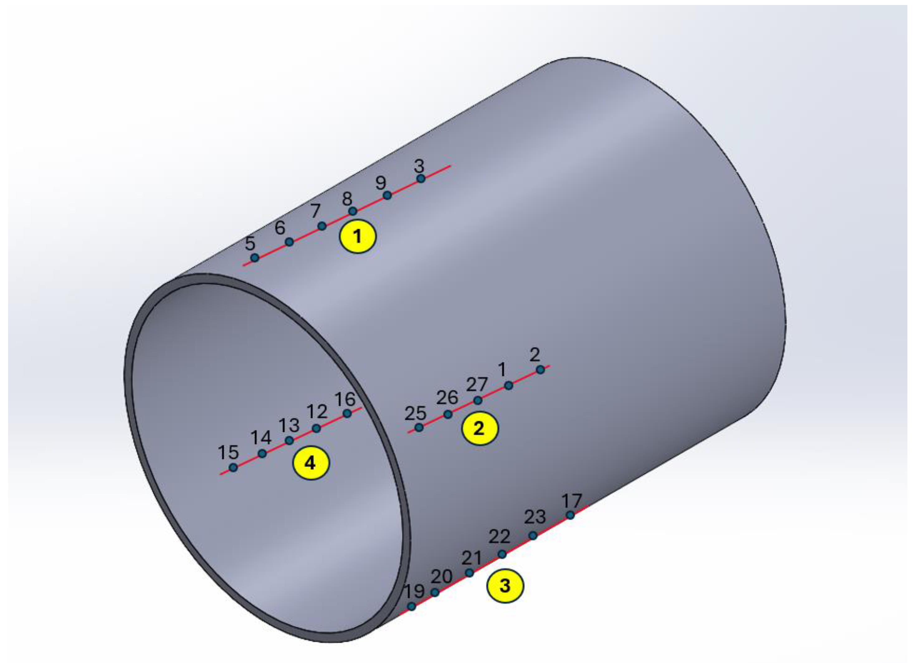
Twelve datasets were used in this study, all obtained from a single-stage, low-speed axial compressor with 60 rotor blades operating at 2400 rpm. A total of 27 sensors were installed at various locations on the compressor—26 were pressure sensors, and one was a Hall effect sensor used to measure rotational speed. The sensor layout was chosen based on configurations commonly found in similar experimental setups used in conjunction with this specific compressor [21]. It is important to note that this work does not aim to determine optimal sensor placement. Instead, it focuses on evaluating the performance of the proposed stall prediction method using a fixed, predefined spatial configuration and examines how this arrangement influences the resulting prediction horizon. The sensor locations are shown in Figure 3, with sensors positioned approximately parallel to the blade chord line. In each row, the first sensor is placed just upstream of the blade’s leading edge. The numbered labels correspond to column indices in the dataset.
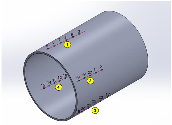
Figure 3.
Labeling of the sensors, where the four blade chords are numbered in yellow.
The data were collected around a flow coefficient that is close to the stall event, therefore providing experimental data sets that lead to stall and sets that did not lead to stall. The sampling frequency of the pressure sensors is 50 kHz.
4.2. Sliding Window and AR Model
One of the objectives of this work is to analyze the flow through a single blade passage and use the pressure data to estimate corresponding AR models. The data collected consist of pressure measurements around the circumference of the compressor; hence, the data were prepared by extracting the pressure values that correspond to a single blade passage while disregarding other blade passages.
The data were grouped into windows of equal size. Starting from the left of the rotor revolution axis, the windows are shifted to the right one step at a time. The purpose of this is to be able to analyze the dynamics and their changes over time in a smaller region rather than averaging the changes in dynamics over the entire data. This is illustrated in Figure 4, where rectangular boxes of different colors indicate that the window starts from the very left of the timeline and moves to the right by overlapping some portion with the previous window while the size of the window remains constant. This means that one window was treated as a single dataset, which is used to extract a corresponding AR model. It would give a parameter vector of size 1 × as shown in Equation (3), and the roots of the parameters from the parameter vector would give eigenvalues. The value of in the AR model is determined using the BIC criteria since it provides the most consistent result among other information criteria.
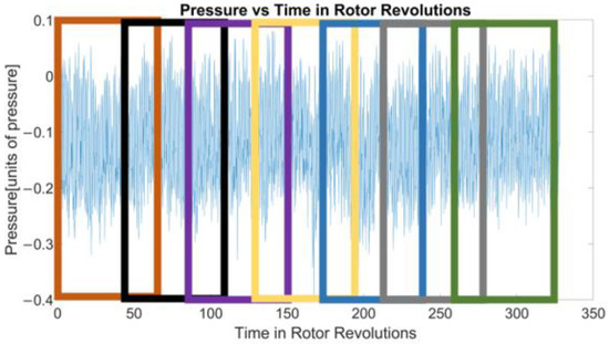
Figure 4.
Sliding windows, the boxes with different colors symbolize the sliding window moving across the pressure data.
The experimental data from the one-stage axial compressor is used along with the outlined information criteria process to determine the order of the assumed AR model structure. The corresponding eigenvalues obtained from the respective AR model for each window are concatenated so that the dynamics of the system are represented by a set of eigenvalues.
4.3. Using GESD for Outlier Detection
The Generalized Extreme Studentized Deviate (GESD) Test is used as an outlier detection method in this research, as it was shown to be one of the most effective outlier detection methods among other methods being compared [22]. The eigenvalues of the continuously identified AR model are evaluated by the GESD algorithm. The purpose of using the growing window algorithm for the analysis of eigenvalue outliers is to build statistical data for outlier detection as well as to localize changes in the time sequence. This is illustrated in Figure 5, where the lines of different colors indicate that the upper bound of the windows keeps moving to the right while the lower bound remains stationary.
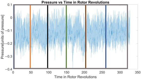
Figure 5.
Expanding windows. The vertical lines of different colors represent the upper bound of the corresponding growing window.
In this work, a fixed maximum number of outliers is used in the GESD algorithm, set arbitrarily to 20. This choice does not influence the identification of stall precursors if the selected value is greater than 1. The purpose of this parameter is not to determine an exact number of anomalies but to track the increasing trend of outliers, which is the critical indicator used for precursor detection. The value of 20 was found to be sufficient to capture this trend without affecting the interpretation of results. This design choice ensures consistent evaluation while maintaining sensitivity to developing instability.
Analogously, the raw pressure data are also evaluated using the GESD algorithm. By comparing the outliers of the raw pressure data and the extracted outliers corresponding to the different AR models (associated with time instances according to the sliding window), an estimated prediction horizon can be formulated.
5. Results
For this research, the datasets contained 26 sets of pressure data. The data points from each sensor of each dataset are analyzed for detecting the precursor of the spike stall using the outliers from the eigenvalues of the computed AR models. The experiments yielded eight datasets having no stall and four datasets with a stall event on a compressor that exhibits spike stall inception. With the given sampling rate and rotor speed, the datasets contain 6560 pressure data points, corresponding to 328 revolutions of the rotor. Since the compressor has 60 blades, each revolution includes multiple blade passages, and the average number of data points per blade passage is 20.
Table 2 presents the results of model order estimation for both test data generated by the AR model (Equation (9)) and real experimental data with varying sample sizes.
Table 2.
Comparison of information criteria for determining the order of AR model.
To validate the effectiveness of the information criteria in estimating the order of an AR model, we first apply them to artificially generated data. This artificial dataset is created using an AR model of known order (p = 3), which allows for controlled evaluation before applying the method to real-world data. The artificial AR model used is defined by Equation (9):
After validating the approach on the artificial dataset, the same process is applied to experimental data obtained from a one-stage axial compressor. The key difference between the two datasets is that the artificial data are generated under controlled conditions with a predefined AR order, while the experimental data come from real measurements, where the true model order must be determined. This distinction is critical in assessing the robustness of the information criteria selection process.
For the test data, the Bayesian Information Criterion (BIC) consistently identifies the correct model order as ‘3’ across all tested cases, aligning with the true order of the AR model. In contrast, the Akaike Information Criterion (AIC) sometimes estimates the correct order but is inconsistent. The order estimated by the Conditional Mean Estimation (CME) method appears highly variable and unreliable.
For the experimental data, AIC’s estimated order fluctuates unpredictably for smaller sample sizes (up to 600), while BIC provides stable estimates. However, the order values determined by BIC for small datasets are too low to capture the pressure data trends accurately. The CME method performs poorly regardless of sample size, producing inconsistent and seemingly random estimates.
When the sample size exceeds 600, the AIC-based order estimation stabilizes at ‘35’, significantly higher than the values estimated for smaller datasets. BIC’s order estimates also increase gradually but remain relatively stable until the dataset length reaches 1500, at which point the estimated order rises slightly. At a sample size of 2000, AIC continues to estimate an order of ‘35’, whereas BIC increases to 27. This suggests that BIC balances computational efficiency with accurate model complexity.
Ultimately, while AIC provides a consistent estimate for large sample sizes, its values suggest potential overfitting. The model order was found to vary between 5 and 7 for most of the experimental data, as estimated by BIC. To ensure a balance between model complexity and accuracy, the more parsimonious order of 5 was chosen.
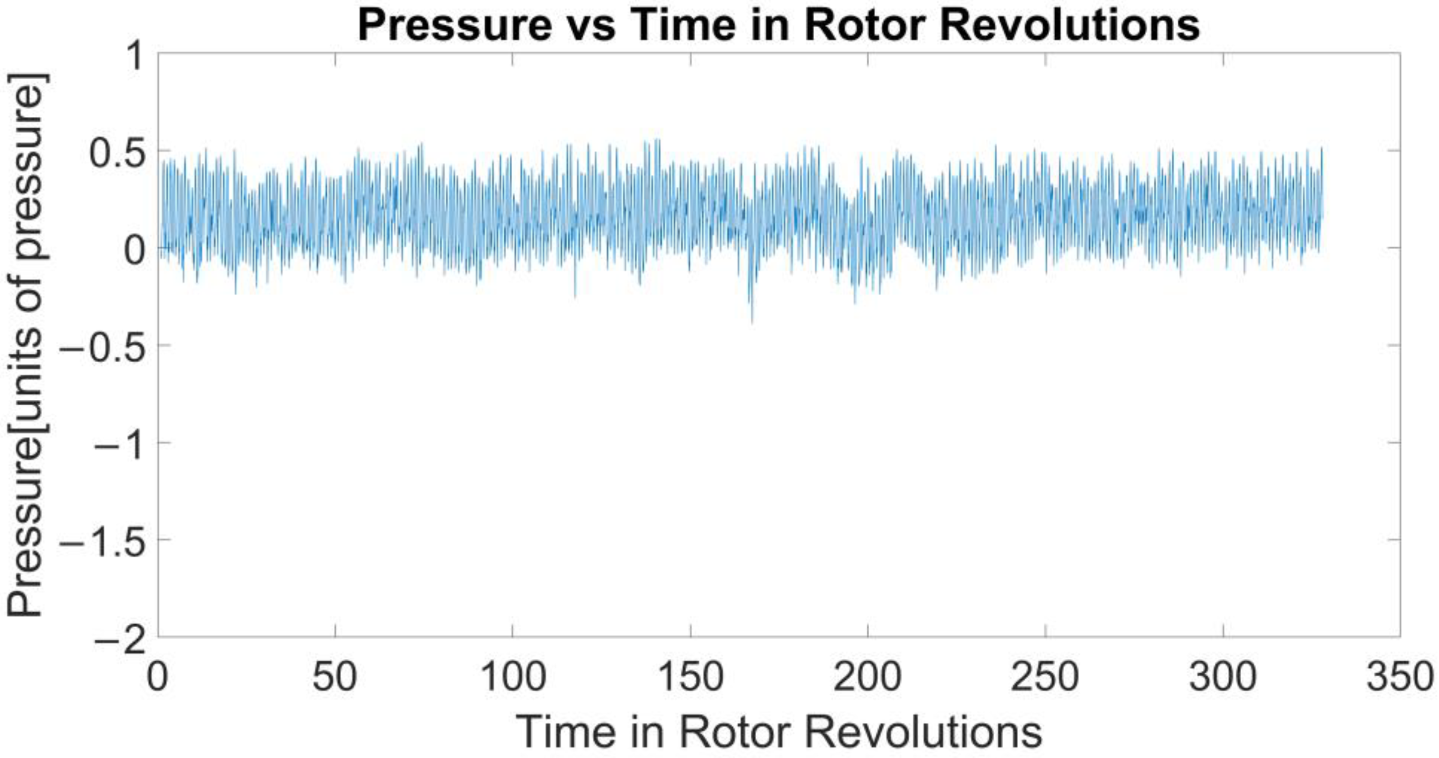
In Figure 6, the pressure data recorded by the sensor do not indicate any outliers, meaning the compressor is running in a normal condition but close to stall. The fluctuations remain stable throughout the time span, suggesting no imminent signs of instability.

Figure 6.
No-stall pressure data plot.
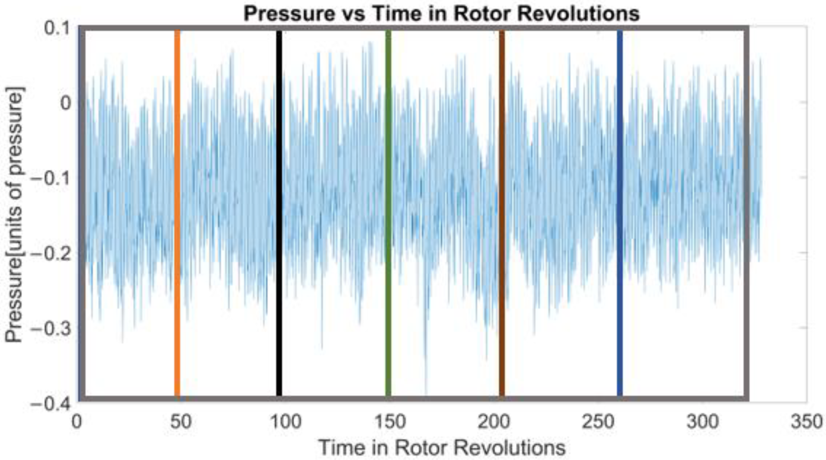
In Figure 7, the pressure remains stable up to approximately 280 rotor revolutions, after which a sudden instability occurs. This marks the onset of a stall event, as seen in the abrupt drop and irregular fluctuations in pressure. Notably, no precursor characteristics are visible in the pressure data before the instability occurs. This highlights a key challenge in spike stall prediction—stall events emerge suddenly without gradual changes in pressure readings beforehand.
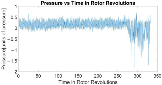
Figure 7.
Stall pressure data plot.
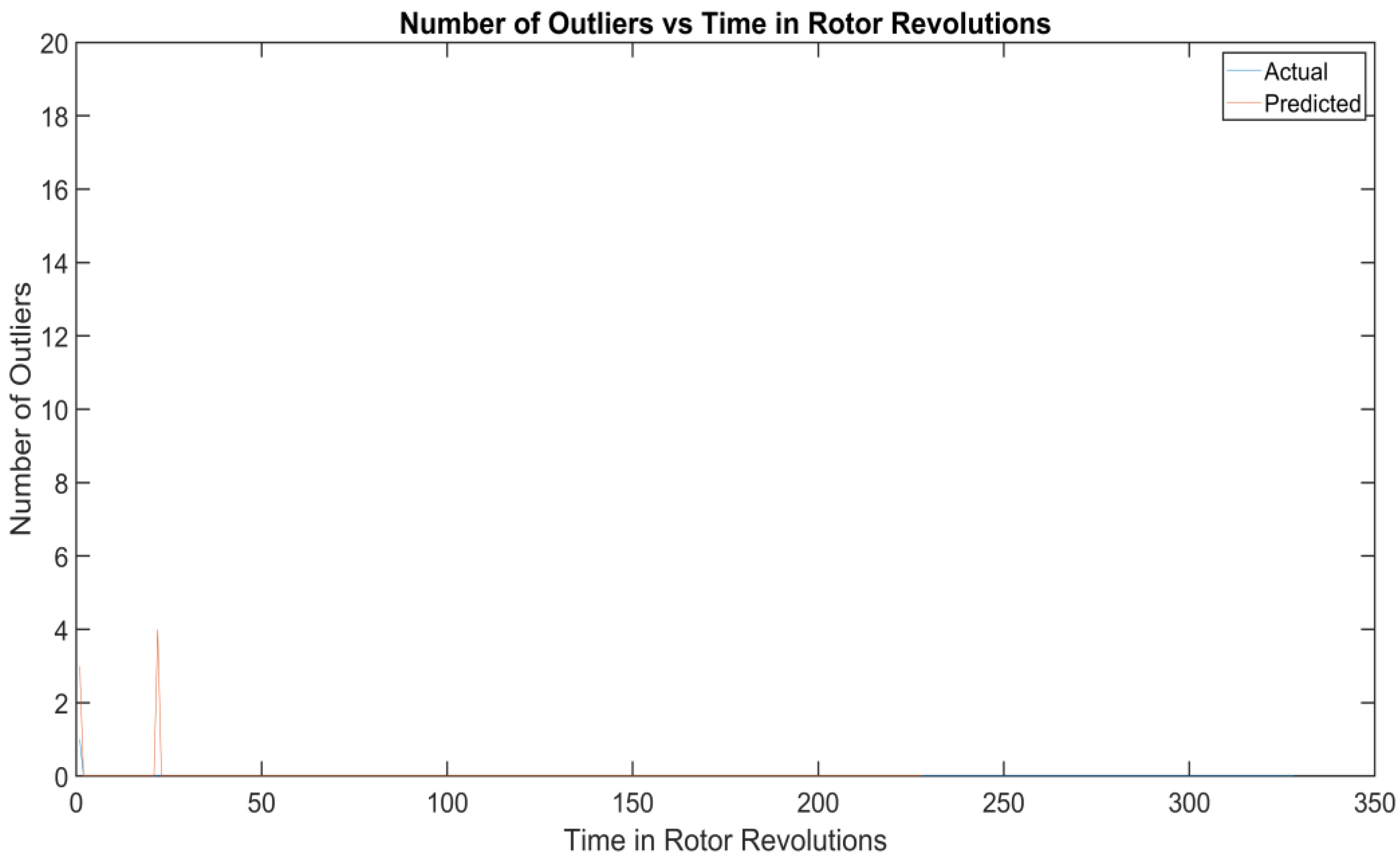
To determine the exact stall onset point, an outlier detection method (GESD) is applied to the pressure data. Since stall-related pressure fluctuations behave as anomalies, the number of detected outliers increases as stall occurs. Figure 8 illustrates this outlier trend: the vertical red line marks the moment the stall occurs, which aligns with the pressure instability seen in Figure 7 at approximately 280 rotor revolutions. This correlation confirms that a rising number of outliers can be used as an indicator of stall onset.
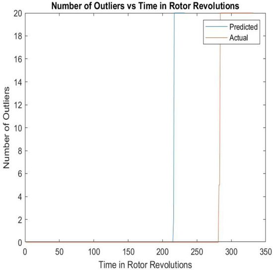
Figure 8.
Outlier detection for stall onset for data shown in Figure 7.
The goal of this research is to predict stall events before they occur. While Figure 7 does not show clear precursors in the pressure data, Figure 8 demonstrates the effectiveness of the proposed AR eigenvalue-based outlier detection method. The blue line in Figure 8, representing outliers identified by the proposed method, shows an increasing trend starting at revolution 204. Similarly, the red line indicates the increasing trend of outliers in the raw data at revolution 281. This implies that using this criterion as a stall precursor, the method can predict stalls 77 revolutions ahead of time, as in this case.
Finally, Figure 9 presents the case where no stall occurs, corresponding to the stable pressure data in Figure 6. As expected, the number of outliers remains consistently low, confirming that when no stall is present, no significant outliers are detected—both in the raw pressure data and in the eigenvalue-based analysis. However, a small initial increase in outliers can be observed at the beginning of the timeline. This is due to regular pressure fluctuations, where the detection method initially starts classifying them as outliers. However, the statistics for classifying them as outliers are insufficient since only a few rotors revolution of data are available. Over time, as the method adapts to normal pressure behavior and has sufficient data points to characterize normal operation, it correctly learns that these fluctuations are not true outliers, and the outlier count stabilizes at zero for the remainder of the timeline.

Figure 9.
Outliers detection for data corresponding to Figure 5.
Out of the twelve experiments, the third, sixth, ninth, and twelfth experiments were performed with stalling conditions. The prediction results of the onset of stalling events in experiments 3, 9, and 12 are shown in Table 3. However, the proposed method employing the identified dynamics did not result in the prediction of the onset of stall in experiment 6. A probable explanation of this shortcoming is explained in Section 6.
Table 3.
Prediction results from the pressure sensors data using AR model. The pressure sensors are arranged as shown in Figure 2.
6. Discussion
The first part of the presented study addresses the determination of the order of AR models using information criteria, where the performance of three different information criteria is compared. From the simulation data model—whose true order is known—the order estimated by BIC is indicated to be the most accurate and the most consistent. Considering the application of information criteria on real experimental data, the order estimated by all investigated information criteria has values varying with the sample size. The performance of BIC, which is observed to be the most consistent initially, also differs with larger variations as the sample size is increased. The application of information criteria does not indicate to be the most reliable method for determining the order of an AR model; however, it provides some reference of the order of the model used for the prediction of the onset of stall in axial compressors.
The results of the proposed stall precursor method are tabulated in Table 3, where the prediction horizon is listed in terms of revolutions, which is the lead time prior to the onset of the stall. It is noteworthy that the prediction is successful in each experiment for the sensors in chord No. 4, making it the most reliable. Additionally, consistency is found with the first and second pressure sensors for all four chords (viewed as in line with the axial flow) and for three of the experiments in predicting stall. The first position pressure sensor in each chord is placed right before the entrance of the rotor blade, before the leading edge of the chord of the rotor blades. Similarly, looking at the average prediction made by the sensors in respective positions in each chord, the average prediction made by the sensors in the first position is 112 revolutions, the second position is 95 revolutions, the third position is 50 revolutions, the fourth position is 72 revolutions, the fifth position is 86 revolutions, and the sixth position is 60 revolutions ahead of the onset of stall. If the prediction average of the first position and second position sensors is considered—as they can be regarded as the most consistent in predicting the onset of stall—the prediction is made 95–112 rotor revolutions ahead. This prediction is earlier than the earliest prediction shown in the literature [10]. However, as discussed in the Results section, the prediction model was not effective for the dataset from experiment 6. Figure 10 shows the pressure variations in a single blade passage for this experiment. It can be observed that the number of pressure data points accumulated (as seen by the number of rotor revolutions) is very limited compared to the amount of data shown in Figure 5 and Figure 6, where the pressure data for two different datasets are shown. For the proposed algorithm to work, the statistics for the outlier detection need to be constructed with sufficient data. Hence, in experiment 6, where stalls occurred much earlier during the experiment, a much smaller data set is available for the calibration of outlier statistics. Consequently, the precursor detection algorithm presented in this paper was inadequate.
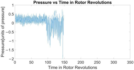
Figure 10.
Experiment 6 pressure plot.
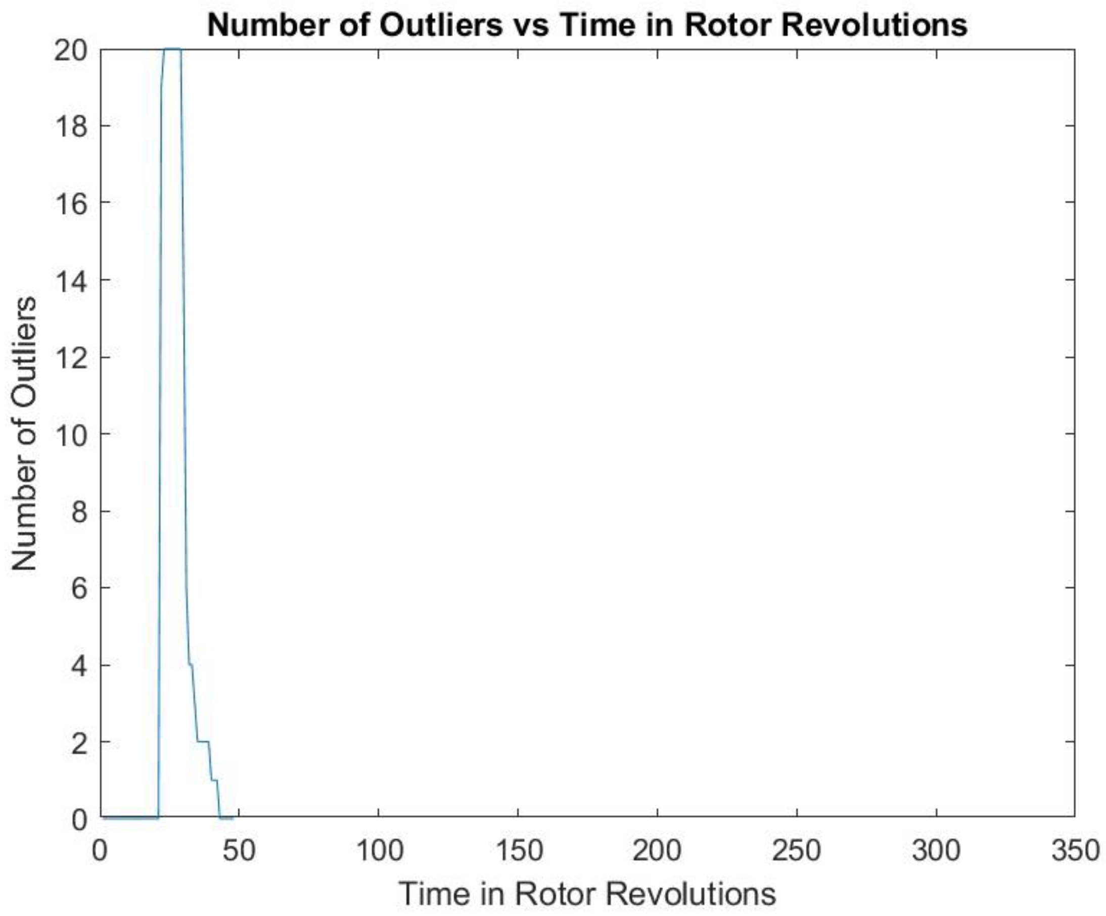
This limitation is further evidenced in Figure 11, where the number of outliers identified by the third eigenvalue declines to zero within a few revolutions after reaching the maximum limit, as the number of data points is insufficient for the computation of the required statistics. To further validate this finding, the data from Experiment 3—in which the model successfully predicted stall—was truncated to match the length of the dataset from Experiment 6, as illustrated in Figure 12. When applying the AR model to the truncated dataset, the prediction outcome mirrored that of Experiment 6, displaying an initial spike in outlier count, which subsequently decayed. The prediction result of the truncated dataset is presented in Figure 13.
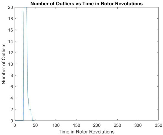
Figure 11.
Outliers from Experiment 6 corresponding to the pressure plot shown in Figure 10.
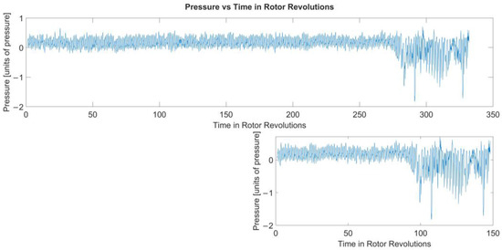
Figure 12.
Experiment 3 pressure plot. The first plot is from the entire data showing pressure in a single blade passage per revolution. The first plot shows the truncated data. The data point up to 200th rotor revolutions from the first plot are cut off during the truncation.
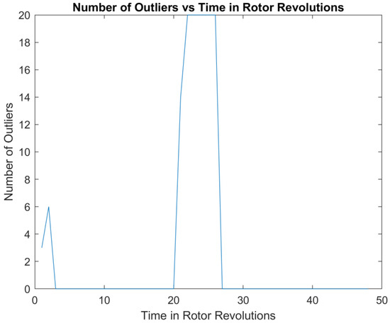
Figure 13.
Outliers from the truncated dataset corresponding to the second plot of Figure 11.
In summary, while the model successfully predicted stall using Sensor 1 data in Experiment 3, it failed to do so when the dataset was truncated to match the length of Experiment 6. This further confirms that the model’s inefficacy in Experiment 6 was primarily due to the limited dataset length, which constrained the statistical framework required for effective stall prediction.
The limitation of utilizing an information criteria in determining the order of an AR model—as shown in this study—indicates a need for further study to address the sample size dependency. This can be achieved by exploring other different model selection methods, such as the k-fold cross-validation. Although this does not affect the proposed method’s results, the model structure and order assumption may play a greater role when the proposed algorithm is employed for different axial compressor geometries.
Additionally, the current study uses a single experimental configuration, and the impact of varying compressor designs—such as multi-stage compressors or different tip clearances—has not been explored. This is a promising area for future research, as these factors may influence the predictive performance of the method. Further studies on compressors with different configurations will help generalize the findings and improve the robustness of the proposed approach.
7. Conclusions
This research investigated the prediction of spike stalls in low-speed axial compressors using dynamic characterization employing autoregressive (AR) models. The order of the model is determined by the application of information criteria through experimentation. The AR model’s characteristics, as expressed by its eigenvalues, are utilized to monitor changes in the flow dynamics as recorded by pressure sensors in the casing aligned with a blade passage. The AR model and its eigenvalues are adaptively estimated using the collected pressure data. Outliers of changing eigenvalues are proposed to function as indicators of change in the flow dynamics, particularly the precursor of spike stalls. The experimental tests reported in this work demonstrated the ability to predict spike stalls up to 112 rotor revolutions prior to the onset of stalls. In addition, for all the experiments where no stalls occurred, the proposed algorithm did not indicate any stall precursors. The spatial information presented by the arrangement of the different pressure sensors is also analyzed. From the limited number of experiments, we conclude that pressure sensors close to—including those just ahead of—the leading edge of the compressor blades have the most sensitivity towards identifying precursors of spike stall events using the proposed algorithm. The results reported in this study also show a larger prediction horizon than what has been reported in the current literature for low-speed axial compressors with spike stall characteristics.
The consistency of the predictions across these datasets mirrors the robustness of the proposed algorithm in various operating conditions. Furthermore, the study highlights several areas for future research, including analysis of data from additional pressure sensors to gain a more comprehensive understanding of the compressor dynamics. Further, alternative methods of determining the order of the AR model could be explored to enhance prediction accuracy for large sample sizes.
Author Contributions
Conceptualization, M.P.S.; Software, A.T.; Formal analysis, A.T.; Resources, J.L.; Data curation, J.L.; Writing—original draft, A.T; Writing—review & editing, M.P.S.; Supervision, M.P.S.; Project administration, M.P.S. All authors have read and agreed to the published version of the manuscript.
Funding
This research was partially funded by the Beijing Natural Science Foundation (JQ24017).
Data Availability Statement
The datasets presented in this article are not readily available because of international collaboration agreements. Requests to access the datasets should be directed to Marco P. Schoen.
Conflicts of Interest
The authors declare no conflicts of interest.
References
- Tan, C.S.; Day, I.; Morris, S.; Wadia, A. Spike-Type Compressor Stall Inception, Detection, and Control. Annu. Rev. Fluid Mech. 2010, 42, 275–300. [Google Scholar] [CrossRef]
- Camp, T.R.; Day, I.J. A Study of Spike and Modal Stall Phenomena in a Low-Speed Axial Compressor. In Volume 1: Aircraft Engine; Marine; Turbomachinery; Microturbines and Small Turbomachinery; American Society of Mechanical Engineers: Orlando, FL, USA, 1997; p. V001T03A109. [Google Scholar] [CrossRef]
- Day, I.J. Axial Compressor Stall. Doctoral Dissertation, University of Cambridge, Cambridge, UK, 1976. [Google Scholar] [CrossRef]
- Day, I.J. Stall, Surge, and 75 Years of Research. J. Turbomach. 2016, 138, 011001. [Google Scholar] [CrossRef]
- Inoue, M.; Kuroumaru, M.; Iwamoto, T.; Ando, Y. Detection of a Rotating Stall Precursor in Isolated Axial Flow Compressor Rotors. J. Turbomach. 1991, 113, 281–287. [Google Scholar] [CrossRef]
- Tryfonidis, M.; Etchevers, O.; Paduano, J.D.; Epstein, A.H.; Hendricks, G.J. Prestall Behavior of Several High-Speed Compressors. J. Turbomach. 1995, 117, 62–80. [Google Scholar] [CrossRef]
- Day, I.J.; Breuer, T.; Escuret, J.; Cherrett, M.; Wilson, A. Stall Inception and the Prospects for Active Control in Four High-Speed Compressors. J. Turbomach. 1999, 121, 18–27. [Google Scholar] [CrossRef]
- Heinlein, G.S.; Chen, J.P.; Chen, C.M.; Dutta, S.; Shen, H.W. Statistical Anomaly Based Study of Rotating Stall in a Transonic Axial Compressor Stage. In Volume 2D: Turbomachinery; American Society of Mechanical Engineers: Charlotte, NC, USA, 2017; p. V02DT46A027. [Google Scholar] [CrossRef]
- Liu, Y.; Li, J.; Du, J.; Zhang, H. Application of wavelet analysis on early stall warning in the axial compressor. In Proceedings of the European Conference on Turbomachinery Fluid Dynamics and Thermodynamics, Lausanne, Switzerland, 8–12 April 2019. [Google Scholar] [CrossRef]
- Aung, E.; Schoen, M.P.; Li, J. Dynamic Characterization and Identification of Flow in a Blade Passage in Near-Stall Conditions of Axial Compressor Systems. In Volume 6: Ceramics; Controls, Diagnostics, and Instrumentation; Education; Manufacturing Materials and Metallurgy; American Society of Mechanical Engineers: Phoenix, AZ, USA, 2019; p. V006T05A013. [Google Scholar] [CrossRef]
- Box, G.E.P.; Jenkins, G.M.; Reinsel, G.C. Time Series Analysis, 3rd ed.; Prentice Hall: Upper Saddle River, NJ, USA, 1994. [Google Scholar]
- Shibata, R. Selection of the Order of an Autoregressive Model by Akaike’s Information Criterion. Biometrika 2023, 63, 117–126. [Google Scholar] [CrossRef]
- Akaike, H. A new look at the statistical model identification. IEEE Trans. Autom. Control 1974, 19, 716–723. [Google Scholar] [CrossRef]
- Hannan, E.J.; Quinn, B.G. The Determination of the Order of an Autoregression. J. R. Stat. Soc. Ser. B Stat. Methodol. 1979, 41, 190–195. [Google Scholar] [CrossRef]
- Burshtein, D.; Weinstein, E. Some relations between the various criteria for autoregressive model order determination. IEEE Trans. Acoust. Speech Signal Process. 1985, 33, 1017–1019. [Google Scholar] [CrossRef]
- Broersen, P. Selecting the order of autoregressive models from small samples. IEEE Trans. Acoust. Speech Signal Process. 1985, 33, 874–879. [Google Scholar] [CrossRef]
- Kay, S. Conditional model order estimation. IEEE Trans. Signal Process. 2001, 49, 1910–1917. [Google Scholar] [CrossRef]
- Chen, H.; Huang, S. A comparative study on model selection and multiple model fusion. In Proceedings of the 2005 7th International Conference on Information Fusion, Philadelphia, PA, USA, 25–28 July 2005; IEEE: Piscataway, NJ, USA, 2005; p. 7. [Google Scholar] [CrossRef]
- Stoica, P.; Selén, Y.; Li, J. Multi-model approach to model selection. Digit. Signal Process. 2004, 14, 399–412. [Google Scholar] [CrossRef]
- Rosner, B. Percentage Points for a Generalized ESD Many-Outlier Procedure. Technometrics 1983, 25, 165–172. [Google Scholar] [CrossRef]
- Lie, J.; Du, J.; Liu, Y.; Zhang, H.; Nie, C. Effect of inlet radial distortion on aerodynamic stability in a multi-stage axial flow compressor. Aerosp. Sci. Technol. 2020, 105, 105886. [Google Scholar] [CrossRef]
- Rosner, B. On the Detection of Many Outliers. Technometrics 1975, 17, 221. [Google Scholar] [CrossRef]


Disclaimer/Publisher’s Note: The statements, opinions and data contained in all publications are solely those of the individual author(s) and contributor(s) and not of MDPI and/or the editor(s). MDPI and/or the editor(s) disclaim responsibility for any injury to people or property resulting from any ideas, methods, instructions or products referred to in the content. |
© 2025 by the authors. Licensee MDPI, Basel, Switzerland. This article is an open access article distributed under the terms and conditions of the Creative Commons Attribution (CC BY) license (https://creativecommons.org/licenses/by/4.0/).