Simplified Data-Driven Models for Gas Turbine Diagnostics

Abstract

The maintenance of gas turbines relies a lot on gas path diagnostics (GPD), which includes two approaches. The first approach employs a physics-based model (thermodynamic model) to convert measurement shifts (deviations) induced by deterioration into fault parameters, which drastically simplify diagnostics. The second approach relies on data-driven models, makes diagnosis in the space of measurement deviations, and involves pattern recognition techniques. Although a thermodynamic model is an essential element of GPD, it has limitations. This model is a complex software critical to computer resources, and the computation sometimes does not converge. Therefore, it is difficult to use the model in online applications. Since the 1990s, we have developed many thermodynamic models for different engines. Since the 2000s, simplified data-driven models were investigated. This paper proposes to substitute a thermodynamic model for novel simplified data-driven models that have the same functionality, i.e., take into consideration the influence of both operating conditions and engine faults. The proposed models are formed and compared with the underlying thermodynamic model. To obtain a solid conclusion about these models, they are verified in twelve test cases formed by three test-case engines, two model types, and two approximation functions. Although the accuracy of the simplified models varies from 1.15% to 0.0082%, it was found acceptable even for the worst case. Thus, these simple-but-accurate models with the functionality of a physics-based model represent a good replacement for the latter. It is expected that the models will stimulate the further development of advanced diagnostic systems.

1. Introduction

Gas Path Diagnostics

Despite the development of renewable energy industries and electrical vehicles, gas turbines remain the principal energy source on earth and the main propulsion system for aviation. In addition to lower operating costs, their continuous monitoring and proper maintenance according to the concept of Engine Health Management (EHM) provide the reduction in fossil fuel consumption and emissions into the atmosphere. As engines evolve in complexity, the need for advanced monitoring systems becomes more urgent.

One of the principal subsystems of a monitoring system carries out diagnosis by using existing gas path measurements (temperatures, pressures, rotation speeds, fuel flow, etc.) and the gas turbine theory (see, for example, [1,2]). Within this paper, such a parametric analysis is called gas path diagnostics (GPD). The area of GPD is well developed and embraces thousands of publications that are thoroughly analyzed, for example, in reviews [3,4,5]. Most of them discuss diagnostic analysis performed using steady-state data [6,7] and static engine models. The totality of these works can be conditionally divided into two main approaches. The first is known as Gas Path Analysis (GPA) and is well described in the works of Volponi [7,8], and the second relies on Artificial Intelligence (AI) methods [9,10,11]. The approaches differ significantly in the use of gas turbine mathematical models. The challenge of GPD is explained by two reasons. First, gas path variables mainly depend on engine operating conditions (power level, ambient conditions, and some others), and the influence of the faults is by far smaller. Second, each fault changes all the variables, and it is a challenge to find the fault on the basis of these changes.

To cope with this problem, GPA transforms these measurement changes (shifts) into shifts of engine component performances (mainly, efficiency, pressure ratio, and flow capacity) using a physics-based gas turbine model. These shifts (fault parameters) determine a fault place, type, and severity, drastically simplifying a final diagnostic statement. Thus, fault parameters form a diagnostic space within the GPA approach. The concept of GPA was introduced by Urban [12] in the early 1970s. He employed a linear diagnostic model that relates measurement changes and fault parameters by an influence coefficient matrix. Since then, to estimate fault parameters many simple analytical solutions within a linear GPA have been provided by using, e.g., matrix inversion, least squares, weighted least squares, and max a-posteriori [8,13]. Unfortunately, as shown in [14,15], the use of the linear model can cause significant additional errors in the estimates. To avoid linearization-induced errors, a nonlinear physics-based model (well known as a thermodynamic model) has been applied since the late 1970s. It was initially employed to compute the matrices for a linear model and for the nonlinear simulation of the impact of different faults on gas path measurements [16,17]. Since the early 1990s, the thermodynamic model and its identification (adaptation) procedure have been an intrinsic part of a nonlinear GPA. One of the first adaptation procedures was proposed in [18]. Then, study [19] performed more complex adaptive modeling with a genetic algorithm, a multi-criteria identification scheme was proposed in [20], and paper [21] introduced an identification concept allowing for sensor faults.

The second approach does not require a complex space transformation. A diagnostic analysis takes place directly in the space of measurement shifts, which is a diagnostic space. Thus, a physics-based model required for the mentioned transformation can be omitted. Data-driven (black-box) models play two roles in the approach. The first role is to provide a reference (performance of a new engine) to compute fault-caused measurement shifts (diagnostic features). Reference models mostly employ Artificial Neural Networks (ANNs) [22,23] or polynomials [23,24] as approximation functions. The second role is to detect and identify engine faults in the space of measurement shifts. Pattern recognition techniques are applied to address this complex issue. The applications of these techniques include, among others, ANNs [25,26,27], Support Vector Machines [26], Principal Component Analysis, the Bayesian approach [28], and Fuzzy Logic [29]. Multilayer Perceptron (MLP) is the most widely applied artificial network for gas turbine fault recognition [6], followed by a radial basis network and a probabilistic neural network [26,28].

Test-bed and field measurements are employed as input data to determine the above-mentioned data-driven models. They are often insufficient, and a thermodynamic model is still involved to help with missing information. For instance, in the benchmarking platform described in [30], a thermodynamic model simulates healthy and faulty engine measurements, which can be used to create reference and fault recognition data-driven models. This nonlinear physics-based model, described, e.g., in [31], utilizes component performance maps, thermodynamic relations in a gas path, and the laws of mass and energy conservation. It allows for computing gas path variables (measured and unmeasured) as a function of operating conditions and fault parameters. Moreover, this physics-based model permits deriving many simplified models. Thus, the thermodynamic model plays a central role in GPD. Many papers are known that report the development and use of the software for gas turbine nonlinear first-principle modeling. Engine manufacturers develop and employ such software for their engines, considering it their proprietary. Similar models were also developed for genetic engines, e.g., a high-bypass two-spool turbofan, for academia and other third parties [30,32]. The GasTurb program developed by Kurzke [33] offers ready-to-use models for many predefined gas turbine configurations. The gas turbine simulation program (GSP) [34] presents a modeling environment for developing new models of different gas turbines. Despite its importance and wide use, a thermodynamic model has some limitations in certain applications. Mathematically, this model presents a high-order system of nonlinear equations numerically solved by an iterative procedure. A nonlinear model identification (adaptation, initialization) procedure for computing fault parameters is organized as an additional external iterative loop. This procedure presents an inverse model, which is characterized by a multiple increase in computing time. Moreover, the iterative loops of the direct and inverse models do not always converge. In addition, the development and use of this complex software with dozens of program modules requires skilled programmers and engine performance engineers. Another difficulty is that the model needs complete information about the performance of all engine components, which is the property of engine manufacturers and is often not available to other parties. The limitations listed above restrict the direct use of thermodynamic models in online and on-board systems, as well as during research, since high-fidelity statistical testing of diagnostic applications sometimes requires millions of model calls.

The shortcomings of the thermodynamic model have stimulated the development of simplified surrogates that do not have convergence issues and have less computer time and memory needs. As mentioned above, the linear diagnostic model has been widely used; however, the linearization causes additional errors. To avoid them, nonlinear data-driven models built on the data generated by thermodynamic models have been proposed. Paper [35] shows that a polynomial-based reference function determined on the data generated by a thermodynamic model provides more accurate diagnostic features than the same function constructed with real measurements. In the same manner, paper [36] demonstrates that ANN-based reference functions determined with thermodynamic model data and real measurements are equally accurate. For online condition monitoring, the authors of paper [37] propose a hybrid reference function composed of ANNs determined on first-principle model data and a Kernel regression-based corrector established with real measurements. The authors validated that this hybrid function can even outperform the underlying model.

The publications mentioned in the previous paragraph confirm the adequacy of substitute data-driven models. However, the research in this area has not been completed: the influence of faults was still simulated by separate linear models. Although our previous conference papers [38,39] propose some data-driven nonlinear models that take into consideration both faults and operating conditions, only particular models for particular engines were studied.

To investigate the proposed class of models in a more general and systematic way, additional model variations were developed for the present paper. This paper analyzes three different engines, two model types (direct and inverse) for each engine, and two approximation functions (polynomials and MLP) for each model type, resulting in twelve model variations. For each model variation, the calculations of errors relative to underlying thermodynamic models were performed. Additionally, for one engine the possible decrease in diagnostic reliability due to the use of the proposed models is estimated. Thus, the present paper verifies the proposed models in a more general and systematic way to draw a convincing conclusion about the applicability of these simple models with the functionality of a complex thermodynamic model. The main motivation for this comprehensive study is to provide advanced real-time diagnostic systems with simple models and in this way contribute to the further development of these systems. We think that such a study completely devoted to the applicability of simplified data-driven diagnostic models is novel: at least reviews [3,4,5] do not mention similar works.

2. Typical Gas Turbine Models

2.1. Thermodynamic Model

Despite there being many known thermodynamic model programs, they all present the same model type that can be characterized as nonlinear physics-based, first-principle-driven, or aero-thermal. It also can be called a component-based model because it computes gas path variables mainly at the input and output of each engine component, and the components are presented by their performance maps. It is a unique model based on physical laws that allows relating gas path variables with engine steady-state operating conditions and the technical state of engine components. Since the model is well described in many papers and is used in most studies on GPD [7], this section only includes a brief model description that will be useful for a better understanding of the present paper. The thermodynamic model can be written by the following structural expression:

$$\overrightarrow{Y}=F(\overrightarrow{U},\overrightarrow{\Theta }),$$

(1)

where a vector $\overrightarrow{Y}$ units gas path variables including measured ones, a vector $\overrightarrow{U}$ consists of operating conditions, and the elements of a vector $\overrightarrow{\Theta }$ are health parameters. The latter can be expressed as $\overrightarrow{\Theta }=\overrightarrow{{\Theta }_0}+\delta \overrightarrow{\Theta }$, where a vector $\overrightarrow{{\Theta }_0}$ corresponds to an engine baseline, and a vector $\delta \overrightarrow{\Theta }$ of fault parameters presents the change in an engine technical state relative to the baseline. To simulate multiple engine deterioration scenarios, these parameters slightly shift each component map in the necessary direction. As mentioned in Section 1, expression (1) is the result of the numerical solution of a model’s nonlinear system. Typically, the Newton–Raphson method is employed.

To find unknown fault parameters within GPA and tune a thermodynamic model to current engine health conditions, an iterative adaptative procedure is applied. This procedure can also be called an adaptative simulation [18] or inverse thermodynamic model. It determines the estimates $\stackrel{\wedge }{\overrightarrow{\delta \Theta }}$ of fault parameters by minimizing the distance between a vector of measurements $\overrightarrow{Y^{\ast }}$ and a vector of model outputs $\overrightarrow{Y}$. Thus, the adaptative simulation solves the following nonlinear minimization problem:

$$\stackrel{\wedge }{\overrightarrow{\delta \Theta }}=\mathit{argmin}‖\overrightarrow{Y^{\mathrm{*}}}-\overrightarrow{Y}(\overrightarrow{U^{\mathrm{*}}},\overrightarrow{{\Theta }_0}+\overrightarrow{\delta \Theta })‖$$

(2)

The resulting dependencies

$$\stackrel{\wedge }{\overrightarrow{\delta \Theta }}=F(\overrightarrow{U^{\mathrm{*}}},\overrightarrow{Y^{\mathrm{*}}})$$

and

$$\overrightarrow{Y}=F\left(\overrightarrow{U^{\mathrm{*}}},\overrightarrow{{\Theta }_0}+\stackrel{\wedge }{\overrightarrow{\delta \Theta }}\right)$$

(3)

can be called an inverse thermodynamic model and an adapted direct model accordingly. As mentioned before, apart from direct use in GPD, a thermodynamic model helps with generating data for creating simplified data-driven models. The subsections below describe two of them, which are the most widely used. The first model is known as an engine baseline model.

2.2. Baseline Model

This model provides a reference for calculating measurement changes caused by engine deterioration. Although a nonlinear physics-based model can serve as a baseline, it is too complex for some diagnostic applications. The employed simplified baseline models determine gas path variables of a healthy engine as a nonlinear function of operating conditions and can be expressed by $\overrightarrow{Y_0}=F\left(\overrightarrow{U}\right)$. This dependency can be built by the approximation of multiple vectors $\overrightarrow{Y_0}=F(\overrightarrow{U},\overrightarrow{{\Theta }_0})$ generated by the physics-based model. Polynomials and MLP are the approximation functions typically employed.

A baseline expression constructed on the basis of second-order full polynomials for one monitored variable and three arguments (operating condition variables) takes the following form:

$$\begin{array}{c}\overrightarrow{Y_{0i}}\left(\overrightarrow{U}\right)=a_1+a_2{u}_1+a_3{u}_2+a_4{u}_3+a_5{u}_1{u}_2\\ +a_6{u}_1{u}_3+a_7{u}_2{u}_3+a_8{u}_1^2+a_9{u}_2^2+a_{10}{u}_3^2,\end{array}$$

(4)

where a₁, …, a₁₀ are determined, for example, by the least squares method.

As to MLP application, Figure 1 illustrates a one-hidden-layer perceptron for computing an engine baseline. The necessary weight coefficients of matrixes W₁ and W₂ are usually estimated by a backpropagation learning algorithm using as outputs physics-based model-generated vectors $\overrightarrow{Y_0}$.

2.3. Linear Diagnostic Model

In contrast to a baseline model, which considers the change in operating conditions, a linear diagnostic model takes into account engine health conditions and presents the linearization of a dependency $\delta \overrightarrow{Y}=F\left(\delta \overrightarrow{\Theta }\right)$. This model calculates a [m × 1]-vector $\delta \overrightarrow{Y}$ of the gas path variable changes (deviations) corresponding to a [r × 1]-vector $\delta \overrightarrow{\Theta }$ of fault parameters based on a [m × r]-matrix of influence coefficients H. Thus, the model presents a system of linear equations:

$$\delta \overrightarrow{Y}=H\delta \overrightarrow{\Theta }.$$

(5)

The most typical way to generate the matrix H is to apply a perturbation methodology to the underlying physics-based model [7]. As the parameters δΘ induced by real deterioration of engine components are not too great (less than 5–7%), the linear model is accurate enough.

2.4. Linear Estimation of Fault Parameters

Once determined, the matrix H allows estimating fault parameters through different methods. When m = r, the solution of system (5) is simple:

$$\stackrel{\wedge }{\overrightarrow{\delta \Theta }}=H^{-1}\delta \overrightarrow{Y^{\mathrm{*}}},$$

(6)

where a vector $\delta \overrightarrow{Y^{\ast }}$ is composed of the engine measurement deviations from the engine baseline induced by faults.

For the case m > r, the following analytical least squares solution provides the estimates with lower errors [8]:

$$\stackrel{\wedge }{\overrightarrow{\delta \Theta }}={\left(H^{T}H\right)}^{-1}{H}^T\delta \overrightarrow{Y^{\mathrm{*}}}.$$

(7)

This solution is the result of the minimization of the distance between the model outputs $\delta \overrightarrow{Y}$ and the measurement deviations $\delta \overrightarrow{Y^{\ast }}$. The increase in the number of measurements required for the least squares method (LSM) can be achieved by installing additional sensors and, more feasible, employing a multipoint diagnostic option.

Estimates given by Equation (7) can be further improved by using a weighted least squares solution [14]:

$$\stackrel{\wedge }{\overrightarrow{\delta \Theta }}={\left(H^{T}WH\right)}^{-1}{H}^{T}W\delta \overrightarrow{Y^{\mathrm{*}}},$$

(8)

where W = R⁻¹ is a weighting matrix, and R presents a measurement covariance matrix. The W matrix allows us to better consider more precise measurements.

If random estimation errors are expected to be too high, the following regularized solution [15] can be obtained:

$$\stackrel{\wedge }{\overrightarrow{\delta \Theta }}={\left({M+H}^{T}WH\right)}^{-1}{H}^{T}W\delta \overrightarrow{Y^{\mathrm{*}}},$$

(9)

where the matrix M represents a priori expected values for health parameter estimation errors [15]. The estimates by Equation (9) proceed from the minimization of either the distance between the model and the measurements or the norm of the fault parameter vector $\delta \overrightarrow{\Theta }$. These estimates are biased but have reduced random errors. The linear solutions given by Equations (6)–(9) can be presented in a general form:

$$\stackrel{\wedge }{\overrightarrow{\delta \Theta }}=D\delta \overrightarrow{Y^{\ast }},$$

(10)

where matrix D, called a diagnostic matrix, is specific for each estimation method. It does not depend on actual measurements and can be determined beforehand. Since the linear solutions do not need a complex nonlinear model and its iterative adaptation procedure, they are still in use. However, the simplicity of the enlisted linear solutions has a cost: the linearization causes additional estimation errors. Kamboukos and Mathioudakis [15] investigated the influence of turbofan model linearization on the accuracy of fault parameter estimation, and they concluded that a linear estimation method could not guarantee the accuracy required.

3. Methodological Considerations

The objective of the present paper is to create and validate simple data-driven models of a new structure that have the accuracy and functionality of an underlying thermodynamic model. It follows from the previous section that new models should be nonlinear and, in contrast to the models given by Equations (4), (5), and (10), each model should be general enough and relate all three groups of variables: $\overrightarrow{Y}$, $\overrightarrow{U}$, and $\overrightarrow{\Theta }$. Since our objective is to investigate a particular diagnostic problem (thermodynamic model substitution by a simplified model) rather than propose a whole diagnostic algorithm in which the models are employed, this paper primarily studies the factors that can affect model accuracy. Since these factors are not known beforehand, different options are considered for each factor, such as the following:

• Engine type and application: three different engines;
• Model types: direct and inverse for each engine;
• Approximation functions: polynomials and MLP for each engine and model type;
• Fault classes: single and multiple for each engine;
• Number of fault classes: specific for each engine.

All possible combinations of these options yield 12 cases of comparison of a simplified model with the underlying thermodynamic model. In every case, the loss of simulation accuracy or diagnostic reliability due to the used simplified model is assessed. If a small loss is observed, this model is considered adequate to the underlying model. The generalization of results from all the comparison cases will allow us to draw sound conclusions about the applicability of simplified models.

As will be shown below, each comparison case includes models with a great number of unknown coefficients (about 200 for polynomials and 1000 for MLP), MLP models are applied to up to 40,000 engine operating points at each learning iteration (epoch), MLP learning lasts about 150 epochs, learning is repeated up to 100 times for a higher precision of the results, and the above calculations should be repeated about 30 times to choose the proper hyperparameters. As a result, the calculation with one hyperparameter value can last up to 10 h (see Section 5.3, Engine 2). Hence, to complete the calculations for all cases within a reasonable time, the following assumptions mainly related to a diagnostic algorithm were made in the present paper:

• The simplified models are obtained at the standard ambient conditions of engine operation. To extend the models to other ambient conditions, the known correction equations can be easily employed [40].
• As engine gas path models are studied, gas path faults are only presented in a diagnostic algorithm. Faults of control and measurement systems are not considered.
• All fault parameters have the same interval of variation.
• Only one well-known pattern recognition technique is used in Section 7 for the analysis of diagnostic reliability with different models employed. The problem of the best technique is not investigated.

The first assumption can really affect the accuracy of the proposed data-driven models. Since a thermodynamic model does not use simplified correction equations, their use for the proposed models will introduce additional errors. However, this issue can be solved by direct inclusion of ambient temperature and pressure in the list of input variables. Since we already have experience of working with seven-to-nine input variables, adding two variables should not present a serious problem. The next three assumptions are mostly related to a diagnostic algorithm, rather than an engine model. They can change the level of diagnostic reliability, but this change will be the same for proposed and thermodynamic models. In this way, the accuracy of the proposed models relative to the thermodynamic model will not be affected.

4. Test-Case Engines

To form the list of test-case gas turbines, the following criteria were taken into consideration: availability of a thermodynamic model, different model designers, and different engine structures and applications. According to these criteria, three test-case engines were chosen:

• Civil aircraft turbofan (Engine 1);
• Helicopter free-turbine engine (Engine 2);
• Industrial power plant (Engine 3).

These three test-case engines allow us to verify the applicability of the proposed simplified data-driven models for different engines. For the first two engines, the necessary data to build and test the simplified models have been obtained through the nonlinear physics-based simulation provided by the software GasTurb 12. The use of this well-known program helped us to have reliable data for building the simplified nonlinear models mentioned, and this will also allow other researchers to repeat the present study. The availability of a thermodynamic model and field recordings explains the choice of the third engine. It is an aeroderivative free-turbine power plant for driving centrifugal natural gas pipeline compressors. The power plant is presented by a thermodynamic model program developed by the authors of the present study. A single run of the program allows generating all necessary data for creating and validating simplified models under different operating and faulty conditions. This reduces the risk of data corruption caused by manually merging data from different sources.

For all the engines, the data were obtained at different operating modes set by the rotation speed variable of a high-pressure turbine (HPT) and under the standard ambient conditions. The rest of the gas path measurements, called monitored variables, are specified in

Table 1. Monitored variables.

No.	Name	Symbol	Engine 1	Engine 2	Engine 3
1	Net thrust	R	x	-	-
2	Shaft power delivered	NLPT	-	x	-
3	Fuel consumption	GF	x	x	x
4	HPC pressure	PC	x	x	x
5	HPC temperature	TC	x	x	x
6	HPT pressure	PHPT	x	x	x
7	HPT temperature	THPT	-	x	x
8	LPT pressure	PLPT	x	x	-
9	LPT temperature	TLPT	x	x	x
10	LPT spool speed	nLPT	-	-	x
	Total number of variables	m	7	8	6–7 *

Notes: 1. For the turboshaft engines (Engine 2 and Engine 3), HPC means a compressor, and LPT means a power turbine. 2. * Varying numbers m = 6–7 for Engine 3 are explained by the different engine control variables established in the calculations. Symbol “x” means “measured”, symbol “-” means “unmeasured”.

separately for each engine. All the variables correspond to real gas turbine measurement systems.

The monitored variables of each engine are computed by the corresponding thermodynamic model with faults embedded. As the fault parameters are input variables in the proposed direct models and output variables in the inverse models, an excessive number of these quantities is required, which can be a challenge. For this reason, only faults of the main engine components (compressors, combustion chamber, and turbines) were selected. The faults of each component are quantified by the parameters δG and δη that shift component flow and efficiency maps.

Table 2. Fault parameters.

No.	Name	Symbol	Engine 1	Engine 2	Engine 3
1	Fan capacity parameter	δGLPC	x	-	-
2	Fan efficiency parameter	δηLPC	x	-	-
3	HPC capacity parameter	δGHPC	x	x	x
4	HPC efficiency parameter	δηHPC	x	x	x
5	HPT capacity parameter	δAHPT	x	x	x
6	HPT efficiency parameter	δηHPT	x	x	x
7	LPT capacity parameter	δALPT	x	x	x
8	LPT efficiency parameter	δηLPT	x	x	x
9	Combustion chamber total pressure recovery coefficient	δσCC	-	-	(x)
10	Combustion chamber efficiency parameter	δηCC	-	-	(x)
	Total number of parameters	r	8	6	8–6 *

Note: * Varying numbers r = 8–6 for Engine 3 are explained by the different fault structures chosen in the calculations. Symbol “x” means “used”, symbol “-” means “not used”.

enlists the parameters chosen for each engine. The proportions m/r = 0.87, 1.33, and 0.75–1.17 between monitored and fault quantities of the analyzed engines characterize their diagnosability. According to these numbers, we can expect that Engine 2 has the highest level of diagnostic reliability, followed by Engine 3 and Engine 1.

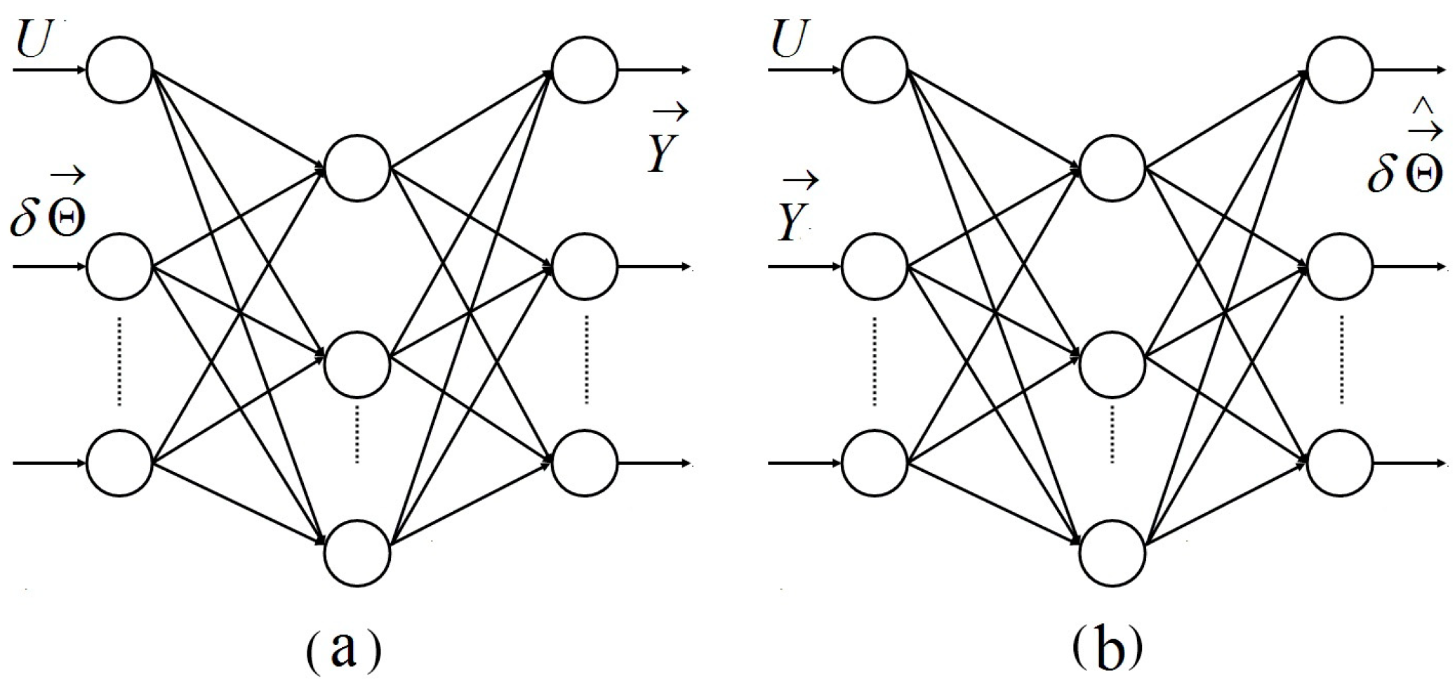
5. Development of Simplified Direct Models

5.1. Polynomial and MLP Model Variations

As mentioned in Section 3, the direct model of each test-case engine will be created by both polynomials and MLP, resulting in six direct model variations in total for the three engines. All of them follow a general expression:

$$\overrightarrow{Y}=F\left(\overrightarrow{\delta \Theta ,}U\right)$$

(11)

The expression is similar to Equation (1) of a thermodynamic model but has one simplification: instead of a whole vector of operating conditions $\overrightarrow{U}$, only one variable U is now included. It is a power set variable that changes an operating mode, while ambient conditions remain fixed (standard). The same variable, high-pressure rotor speed n is chosen as a power set variable U for all the engines. The structure of the vector $\overrightarrow{\delta \Theta }$ is specific to each engine and determined by Table 2.

The polynomial and MLP-based model variations in each engine are included in a specific testing MATLAB-2024 program and always use the same input data for each case of comparison. This guarantees an accurate comparison of the polynomials and MLP.

Based on our previous experience [23,35,38,39], second- and third-order polynomial functions were employed. As to MLP, its scheme is given in Figure 2a. The perceptron was created, learned, and simulated using the MATLAB-2024 Neural Network Toolbox. For all engines, the perceptron has one hidden layer, tansig and logsig transfer functions, and trainrp or trainbr learning algorithms with the EarlyStopping option.

5.2. Polynomial Models

5.2.1. Engine 1

Since the model given by Equation (11) has nine independent variables for Engine 1 (eight fault parameters from Table 2 and a power set variable), the number of the polynomial unknown coefficients for each dependent variable can be 50 and greater. To have sufficient flexibility, MLP will have a great number of coefficients as well. Therefore, numerous input data are required to estimate the coefficients of both approximation techniques.

To generate these data for Engine 1, seven variables typically used for monitoring (see Table 1) were simulated by the GasTurb turbofan model at five operating modes given by relative speeds of a high-pressure spool: n = 1.0, 0.9, 0.8, 0.7, and 0.6. At each mode, 719 operating points with different values of the eight fault parameters from Table 2 were simulated. These values were randomly distributed within the interval (0.0, +0.05) for the flow parameters δA_HPT and δA_LPT and the interval (0.0, −0.05) for the others. The totality of 3595 operating points was divided into a learning set (85%) and a validation set (15%).

To choose the best polynomial configuration, two structures of polynomial functions and a normalization option were examined. The first structure includes a full second-order polynomial for the eight δΘ-arguments and the following independent n-members: “n”, “n²”, “n³”, and “n⁴”. This results in k = 49 unknown coefficients. This structure looks like the following:

$$\begin{array}{c}Y\left(\delta \overrightarrow{\Theta },n\right)=a_1+a_2\delta {\theta }_1+a_3\delta {\theta }_2+\cdots +a_9\delta {\theta }_8\\ +a_{10}\delta {\theta }_1\delta {\theta }_2+\cdots +a_{37}\delta {\theta }_7\delta {\theta }_8+a_{38}\delta {{\theta }_1}^2+\cdots \\ +a_{45}\delta {{\theta }_8}^2+a_{46}n+a_{47}{n}^2+a_{48}{n}^3+a_{49}{n}^4\end{array}$$

(12)

The n-members up to the fourth-order polynomial are necessary to accurately approximate the influence of the rotating speed at five operating modes. The second polynomial structure presents a full second-order polynomial of nine δΘ and n arguments. The following expression with k = 57 members describes it:

$$\begin{array}{c}Y\left(\delta \overrightarrow{\Theta },n\right)=a_1+a_2\delta {\theta }_1+a_3\delta {\theta }_2+\cdots +a_9\delta {\theta }_8+\\ a_{10}n+a_{11}\delta {\theta }_1\delta {\theta }_2+\cdots +a_{46}\delta {\theta }_{8}n+a_{47}\delta {{\theta }_1}^2+\cdots \\ +a_{55}{n}^2+a_{56}{n}^3+a_{57}{n}^4\end{array}$$

(13)

As to the normalization, it was performed for each monitored variable Y by dividing an actual value corresponding to an engine with introduced faults by the value of the same variable at the same operating mode of a healthy engine.

For all four polynomial model variations, the coefficients were estimated by the least squares method.

Table 3. Polynomial structures and errors (direct models).

Engine 1
Polynomial	Second order, k = 49	Second order, k = 57
Errors (without normalization)	0.142018	0.027771
Errors (with normalization)	0.030626	0.011448
Engine 2
Polynomial	Second order, k = 38	Third order, k = 100
Errors	0.004601	0.004406
Engine 3
Polynomial	Second order, k = 37	Third order, k = 99
Errors	0.000817	0.000715

contains the accuracy performances (mean values of the RMSE of all variables). In the upper part of the table, the Engine 1 model variations are given. As can be seen in the table, the polynomial structure with 57 coefficients applied to the normalized variables is the most accurate. It will be used in further comparisons.

5.2.2. Engine 2

As with the Engine 1 models, the data necessary for creating polynomial and MLP-based models of Engine 2 were simulated by the GasTurb turboshaft model at five operating modes determined by high-pressure spool speeds: n = 1.0, 0.9, 0.8, 0.7, and 0.6. For each mode, eight monitored variables (see Table 1) were computed at 1458 operating points corresponding to different fault parameters (see Table 2) distributed like the Engine 1 parameters. As before, 85% of the total 1458 × 5 = 7290 points constitute a learning set, and 15% of the points form a validation set.

Before the comparison with MLP, three polynomial structures were verified. Since the number of independent variables of Engine 2 models is significantly lower than that of Engine 1 models (seven against nine), a full third-order polynomial function $fp3\left(\delta \overrightarrow{\Theta },n\right)$ with 99 unknown coefficients is now considered in addition to the full second-order function and $fp2\left(\delta \overrightarrow{\Theta },n\right)$ (36 coefficients) applied to the Engine 1 models. Considering n-members, two corresponding model structures look like

$$Y\left(\delta \overrightarrow{\Theta },n\right)=fp2\left(\delta \overrightarrow{\Theta },n\right)+a_{37}{n}^3+a_{38}{n}^4$$

(14)

and

$$Y\left(\delta \overrightarrow{\Theta },n\right)=fp3\left(\delta \overrightarrow{\Theta },n\right)+a_{100}{n}^4.$$

(15)

As with Engine 1, the variables Y from all operating points were normalized and used by the least squares method for estimating coefficients of the compared models. Since the number of independent variables is smaller, and the volume of input data is greater than those of Engine 1, we can hope that the Engine 2 models will be more accurate. Indeed, in Table 3, which presents the accuracy performances of these models, one can see that the Engine 2 models are more accurate than the Engine 1 models. We also can state that the model with the third-order polynomial function (Equation (15)) exposes the best performance. It has been selected for further comparison.

5.2.3. Engine 3

The input data for determining Engine 3 polynomial and MLP-based models were generated by a thermodynamic model developed by the authors.

Since the simulated power plant with a free turbine was simulated with its mechanical load, the centrifugal compressor, the plant has one degree of freedom and needs one variable to set its regime. The high-pressure spool speed variable was chosen, and four regimes were set by its values 10,900, 10,702, 10,500, and 10,200 r/min. At each regime, 10,000 operating points with six randomly distributed fault parameters (see Table 2) were simulated, resulting in 40,000 total points (5.5-times greater than for Engine 2) divided into learning and validation sets in the same proportion of 85% to 15%. All the data were generated automatically, thus excluding manual data processing errors. Additionally, the convergence of a model system solution was controlled, and only correct data were recorded. The above measures promise a higher approximation accuracy for polynomial and MLP-based Engine 3 models.

Since the number of seven independent variables did not change compared with Engine 2, the second- and third-order full polynomials are used. As the input data correspond to four operating models, the n⁴-member is excessive now. Thus, the Engine 3 polynomial structures can be written by

$$Y\left(\delta \overrightarrow{\Theta },n\right)=fp2\left(\delta \overrightarrow{\Theta },n\right)+a_{37}{n}^3$$

(16)

and

$$Y\left(\delta \overrightarrow{\Theta },n\right)=fp3\left(\delta \overrightarrow{\Theta },n\right)$$

(17)

and have 37 and 99 unknown coefficients accordingly. The bottom part of Table 3 contains the performances of these structures. As can be seen, the third-order polynomials have lower errors, and therefore they have been chosen for further comparison with MLP.

5.3. MLP-Based Models

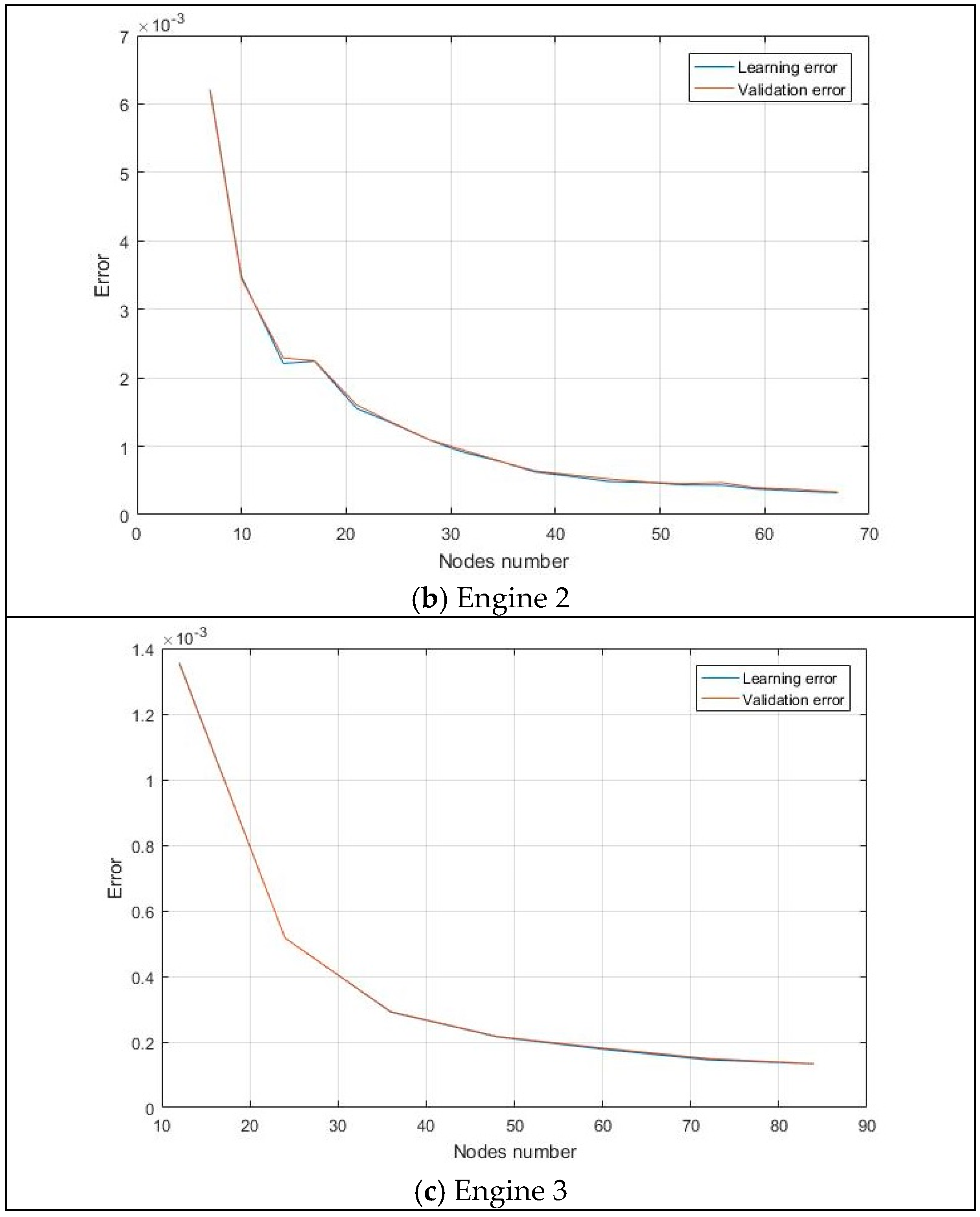
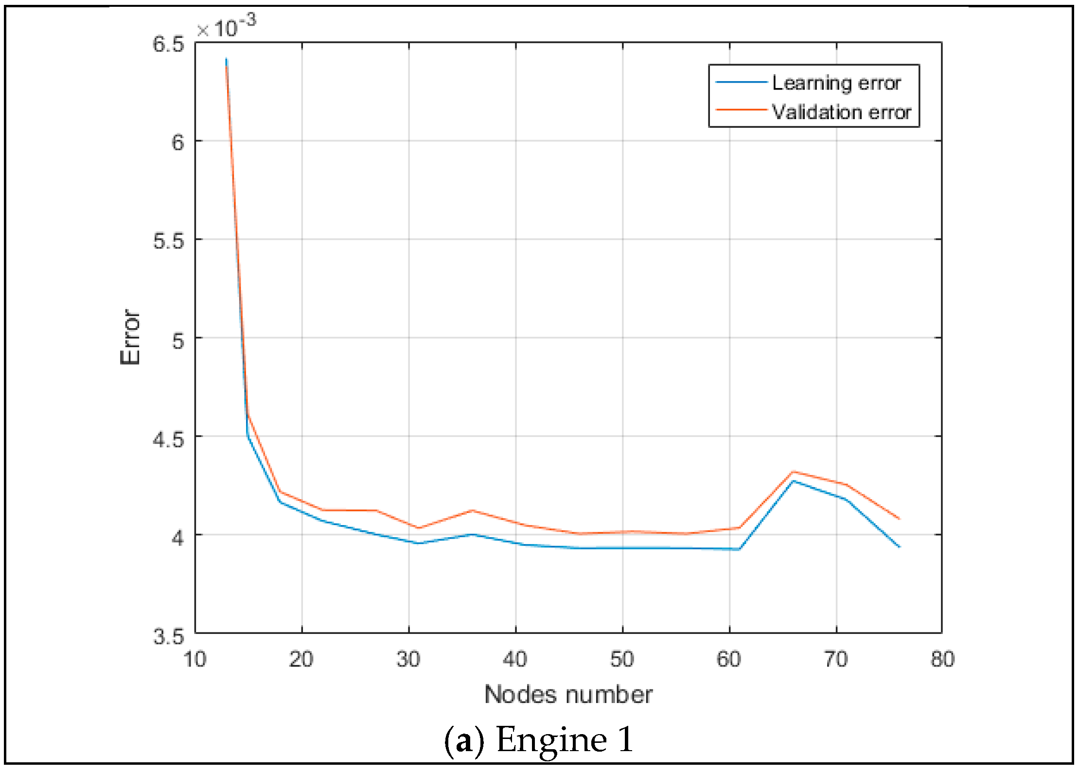
5.3.1. Engine 1 MLP Model

All MATLAB–2024 training functions in the application to diagnostic tasks were verified in our previous study [41], and rainrp (resilient backpropagation) was found the most accurate. Nevertheless, for inverse engine models [42] the trainbr function (Levenberg–Marquardt optimization with Bayesian regularization) was better. Since the choice of the best learning algorithm varies depending on the problem to solve, the experiments with rainrp and trainbr were repeated. Figure 3 illustrates a typical learning process by each algorithm. We can see that the trainbr algorithm yields a by-far-higher accuracy since it does not stay too long in local minimums (as exposed in Figure 3b). Thus, further learning of direct models of all the engines uses the trainbr algorithm.

When a learning algorithm is chosen, the next step is to determine the criterion to stop the algorithm. There are three options: to set a maximum number of epochs, to set a minimum network error, or EarlyStopping, which optimally stops the algorithm to avoid an overfitting effect. Since EarlyStopping allows a reduction in the number of hyperparameters and it operated correctly in our previous experiments, the present study also employs this option.

As the number of input and output nodes is determined by the given structure of the vectors $\overrightarrow{Y}$ and $\overrightarrow{\delta \Theta }$, the number of hidden-layer nodes is the unique hyperparameter. To choose its optimal value, the computations of the Engine 1 MLP-based direct model were performed with different values. Since the computation is affected by random factors (random distribution between learning and validation data and random initial values of network coefficients), the model errors also have random uncertainty. To reduce it, the calculation for each number of nodes was repeated k_iter = 10 times, and the average error was estimated. Appendix A Figure A1a plots these average accuracy parameters, which help to find the optimal node number 54 corresponding to the highest MLP accuracy.

Table 4. Polynomial and MLP errors (direct models).

Monitored Variables	Polynomials		MLP
	Learning	Validation	Learning	Validation
Engine 1 (polynomial: k = 57, MLP: k = 925)
R	0.04099	0.04287	0.00200	0.00244
GF	0.01148	0.01184	0.00098	0.00110
PC	0.00911	0.00929	0.00070	0.00077
TC	0.00121	0.00125	0.00019	0.00020
PHPT	0.01008	0.01033	0.00074	0.00084
PLPT	0.00539	0.00550	0.00035	0.00039
TLPT	0.00550	0.00556	0.00060	0.00069
Mean	0.011083	0.011448	0.000759	0.000874
Engine 2 (polynomial: k = 100, MLP: k = 1080)
NLPT1	0.01607	0.01631	0.00096	0.00096
GF	0.00536	0.00549	0.00046	0.00049
PC	0.00322	0.00334	0.00019	0.00020
TC	0.00051	0.00051	0.00009	0.00009
PHPT	0.00440	0.00452	0.00021	0.00022
THPT	0.00259	0.00263	0.00029	0.00031
PLPT	0.00044	0.00044	0.00003	0.00003
TLPT	0.00257	0.00259	0.00029	0.00029
Mean	0.004400	0.004482	0.000319	0.000329
Engine 3 (polynomial: k = 99, MLP: k = 1267)
GF	0.00140	0.00140	0.00020	0.00022
PC	0.00029	0.00029	0.00010	0.00010
TC	0.00020	0.00020	0.00005	0.00005
PHPT	0.00085	0.00084	0.00013	0.00013
THPT	0.00060	0.00060	0.00013	0.00014
TLPT	0.00057	0.00058	0.00012	0.00012
nLPT	0.00027	0.00027	0.00008	0.00008
Mean	0.000713	0.000715	0.000132	0.000134

helps to compare the accuracy of the best polynomial and MLP-based Engine 1 direct models. The table contains the Root Mean Square Errors (RMSEs) of all monitored variables and their mean value. This information allows us to make the following statements:

• − The accuracy of the variables differs a lot. However, for all computational cases (learning and validation of both approximation techniques), the accuracy rank is conserved as the same from the most accurate compressor temperature TC to the least accurate thrust R.
• − The validation errors are larger, but very close to the learning errors for each case and variable. This is the confirmation of the correctness of a whole learning process. For all the cases and variables, MLP has a by-far-higher accuracy.

The MLP superiority is mainly explained by a 2.26-times-higher number of unknown coefficients: 122 per variable Y, against only 57 polynomial coefficients. In general, the Table 4 data confirm that the MLP-based direct model of Engine 1 has acceptable accuracy because its approximation errors are considerably smaller than typical measurement errors of the corresponding variables. Theoretically, the performance of polynomials can be enhanced by selecting a full third-order structure. However, such a function of nine arguments will be complex and, so far, it is not considered for Engine 1.

The calculation of each case was repeated 10 times, and the error in Table 4 presents an average value with a lower uncertainty. The level of this uncertainty is generally proportional to the error itself. The ratio of a 3σ-uncertainty amplitude to the error itself varies from 6% to 37% for polynomials and from 23% to 50% for MLP. That is, all Table 4 numbers are statistically significant. As a result, mean validation errors can be presented with 3σ-confidence as 0.011448 ± 0.00192 for polynomials and 0.000874 ± 0.00027 for MLP.

5.3.2. Engine 2 MLP Model

As the origin of input data for Engine 2 and Engine 1 simplified models is the same, the volume of data for Engine 2 does not differ a lot from the Engine 1 data. Since the number of input variables does not vary significantly, the Engine 2 network is similar to the Engine 1 network. That is, MLP has one hidden layer and is learned by the trainbr algorithm with the EarlyStopping option.

To determine the optimal number of hidden-layer nodes, numeric experiments with different numbers have been performed. As before, to enhance the precision the calculation with each number of nodes has been repeated 10 times and average mean errors were determined. Figure A1b plots these errors as a function of the number of nodes. The figure clearly shows that the learning and validation errors drop with each increment in the nodes, and the smallest error corresponds to the largest number of 67 nodes. In this way, MLP with 67 hidden nodes is considered the best and will be considered for the next comparisons. The behavior of the plots supposes further error reduction for the numbers greater than 67. However, so far these numbers are not considered given that the calculation with the number 67 already lasts 10 h (Dell desktop with CORE i7 ninth-generation processor).

For the best configurations of the polynomial and MLP models of Engine 2, the intermediate part of Table 4 includes the RMSEs of the monitored variables estimated on learning and validation operating points and the mean value of these RMSEs. The absolute uncertainty of the presented polynomial and MLP were found to be comparable. In a relative form, 3σ-amplitudes vary for different variables, from 5% to 11% for polynomials and from 40% to 90% for MLP (validation results). As a result, mean validation errors with 3σ-confidence scatter can be presented as 0.004482 ± 0.000214 for polynomials and 0.000329 ± 0.000206 for MLP. Since uncertainty does not exceed 100%, the Table 4 numbers are statistically significant.

The table data help to draw the following statements, which are similar to the statements made for Engine 1 models:

• The accuracy rank of variable Y is conserved as the same in the four computational cases presented.
• The closeness of the validation and learning errors confirms the correctness of a whole learning process.
• For all the cases and variables, MLP has a by-far-higher accuracy, and the mean errors are about 13-times smaller.

Although the polynomial model now uses the third-order functions, and the number of coefficients for one variable Y has increased to 100, the polynomial accuracy is still by far lower than the MLP accuracy. The MLP dominance cannot now be completely explained by a greater number of MLP coefficients because the relation between MLP and polynomial coefficients has now reduced to 1.49 against 2.26 for Engine 1 models. Thus, we can suppose that the MLP approximation functions will be more flexible and accurate, although with a similar number of unknown coefficients as in polynomials.

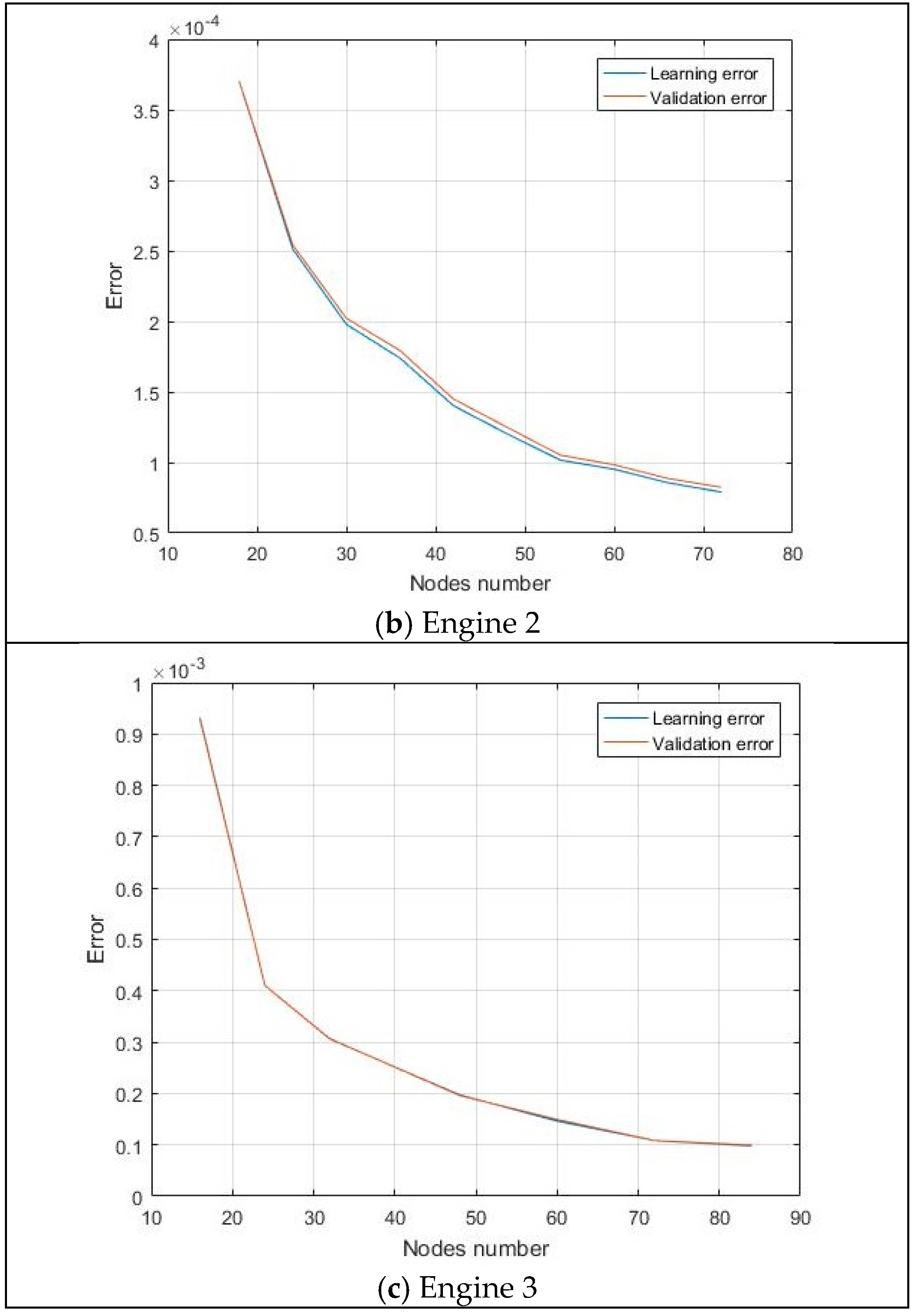
5.3.3. Engine 3 MLP Model

The general MLP structure and options used for Engine 1 and Engine 2 models are conserved for Engine 3: one hidden layer, the trainbr learning algorithm, and EarlyStopping.

As before, experiments with different numbers of nodes were carried out. The plots of Figure A2c illustrate the resulting learning and validation mean errors. As the volume of input data has drastically increased, and the calculation with each node number was repeated 10 times for estimating average values of mean errors, the learning and validation curves are without random perturbations and practically coincide. Therefore, it is clearly seen that the best result corresponds to the maximum number 84, and MLP with this number of nodes is accepted as the best. The plots also show that a better result is possible with a greater number of nodes. However, such a possibility has not been considered so far because each increment in node number causes a significantly larger computation time, and for the number 84 the time already makes up 36 h.

Table 4 shows that the Engine 2 MLP-based model is approximately 2.7-times more accurate compared with the Engine 1 model. In turn, the Engine 3 model outperforms the Engine 2 model by 2.5 times. As before, MLP is by far more accurate than polynomials. However, even the polynomial errors are already significantly smaller than the measurement errors.

The MLP-based model now has very small errors, and the polynomial model approximation errors are already smaller than the measurement errors.

As to the precision of the Engine 3 model data, the absolute uncertainty intervals have reduced proportionally to approximation errors themselves in comparison with the Engine 2 model data, and the relative uncertainty has not changed. The mean validation errors can now be written with a 3σ-confidence probability as 0.000715 ± 0.000015 for polynomials and 0.000134 ± 0.000048 for MLP. Thus, the Engine 3 results are statistically significant.

6. Inverse Models for the First Approach

6.1. Polynomial Models

6.1.1. Engine 1 Inverse Model

During the experiments with polynomials, it was found that the use of absolute values of the monitored variables as arguments of the polynomial functions causes even more serious numerical problems than in the direct models where these variables were resulting functions. They are related to the great difference between the levels of polynomial members, especially when the members have the second- and third-order of the variables. When trying different modes to normalize the arguments, the normalization relatively the values at the highest regime of the healthy engine was found the most accurate.

Table 5. Polynomial structures and errors (inverse models).

Engine 1
Polynomial	Second order, k = 57	Third order, k = 169
Learning Errors	0.004306	0.003555
Validation Errors	0.004368	0.00377
Engine 2
Polynomial	Second order, k = 57	Third order, k = 169
Learning Errors	0.001049	0.0002250
Validation Errors	0.001058	0.0002332
Engine 3
Polynomial	Second order, k = 46	Third order, k = 136
Learning Errors	0.000272	0.000158
Validation Errors	0.000271	0.000159

in its upper part contains the mean accuracy parameters of the polynomials after such normalization. As with the direct models, these data were obtained by repeating the calculation process 10 times with different random learning and validation sets and subsequently averaging the errors. As a result, the computational uncertainty in error estimations is significantly lower than the errors themselves: 3σ-intervals make up on average 0.00035. The acceptable precision of the table data allows us to draw the following conclusions. First, as the differences between learning and validation accuracy are small, the corresponding input data always have the same distributions, i.e., there are no perturbations in data generation. Second, the accuracy of the third-order polynomials is considerably better. Therefore, they are chosen for the next comparison with neural networks.

6.1.2. Engine 2 Inverse Model

As for Engine 1, normalization was applied to the arguments of Engine 2 polynomials, and the calculations were repeated 10 times. Table 5 contains the mean accuracy parameters of the polynomials after such normalization. These results have low computational uncertainty: 3σ-intervals make up on average 0.00010. Comparing the Engine 2 and Engine 1 data in Table 5, one can state that both second-order and third-order Engine 2 polynomials are significantly more accurate than Engine 1 ones. It is also observable that the superiority of the third-order polynomials over second-order polynomials is now more visible: 4.54 times against 1.16 for Engine 1. Thus, these higher-order polynomials will be used for a subsequent comparison with the perceptron.

6.1.3. Engine 3 Inverse Model

The normalization was conserved for the Engine 3 inverse polynomial model. However, the calculation repetitions and averaging over the results were not realized, because of the too-long computation time (about 70 h for 10 repetitions) due to the huge volume of the input data (40,000 operating points). Therefore, the Engine 3 data in Table 5 correspond to one calculation. However, the resulting precision is as high as for Engine 1 and Engine 2 because of the same reason: a significantly greater number of operating points.

For Engine 3, further accuracy enhancement is observed in Table 5: the third-order polynomials are now almost 50% more accurate. As before, they will be compared with MLP.

6.2. MLP-Based Models

6.2.1. Engine 1 Inverse MLP Model

The dependence of the accuracy of the Engine 1 MLP from the hidden nodes number is shown in Figure A2a. It helps to choose 51 as the optimal number of nodes, and the corresponding perceptron is below compared with the polynomials.

The upper part of

Table 6. Polynomial and MLP errors (inverse models).

Fault Parameters	Third-Order Polynomials		MLP
	Learning	Validation	Learning	Validation
Engine 1 (polynomial: k = 169, MLP: k = 875)
δGLPC	0.01209	0.01274	0.01222	0.01254
δηLPC	0.00516	0.00555	0.00537	0.00548
δGHPC	0.00135	0.00149	0.00193	0.00198
δηHPC	0.00208	0.00289	0.00236	0.00239
δAHPT	0.00013	0.00015	0.00126	0.00129
δηHPT	0.00111	0.00122	0.00162	0.001644
δALPT	0.00376	0.00385	0.00387	0.00388
δηLPT	0.00274	0.00287	0.00284	0.00293
Mean	0.003554	0.003769	0.003936	0.004018
Engine 2 (polynomial: k = 169, MLP: k = 1158)
δGHPC	0.000221	0.000227	0.000091	0.000095
δηHPC	0.000173	0.000177	0.000065	0.000068
δAHPT	0.000119	0.000123	0.000078	0.000081
δηHPT	0.000119	0.000121	0.000049	0.000051
δALPT	0.000261	0.000272	0.000094	0.000098
δηLPT	0.000457	0.000479	0.000097	0.000102
Mean	0.0002250	0.0002332	0.0000790	0.0000824
Engine 3 (polynomial: k = 136, MLP: k = 1260)
δGHPC	0.000136	0.000137	0.000088	0.000090
δηHPC	0.000212	0.000213	0.000105	0.000106
δAHPT	0.000016	0.000016	0.000108	0.000127
δηHPT	0.000010	0.000010	0.000078	0.000076
δALPT	0.000236	0.000237	0.000107	0.000109
δηLPT	0.000175	0.000177	0.000098	0.000098
Mean	0.000158	0.000159	0.000098	0.000099

helps to compare these approximation techniques by providing their detailed accuracy performances. One can see that the errors of both techniques are similar for all estimated fault parameters, but the polynomials are slightly more accurate. The precision (3σ-uncertainty intervals) of the presented parameter errors makes up an average of 0.00090. Since a typical range of the parameters in modeling and diagnostic tasks is about 0.0–0.05, the errors themselves presented in the table and their precision can be considered as acceptable for all parameters, except the estimate δΘ₁ (as can be seen in Table 2, it is a fan capacity parameter). Its abnormally high errors are explained below.

Figure 4 and Figure 5 shed some light on the problem of the estimation of parameter δΘ₁. Operating points 1 through 3595 are here presented subsequently for operating modes 1-to 5. Figure 4a shows that the general behavior of the estimates of δΘ₁ is abnormal for modes 2-to 4 (operating points 720-to-2876). Figure 4b more clearly illustrates this phenomenon: in the left side of the plot corresponding to mode 1, the estimates follow well to the true values, but from point 720 (mode 2) they change a little around a mean value of 0.025 and do not react on the true values. In contrast, as can be seen in Figure 5, the estimates of the other fault parameters conserve adequate behavior for all operating points. We see two possible explanations for this phenomenon. First, the influence of δΘ₁ on the monitored variables significantly changes at different operating modes. Second and more probable, there is a shift in the input data between the parameter δΘ₁ and monitored variables at modes 2-to-4. This shift can be caused by a manual manner of forming input data. Anyway, the problem is not critical given that fan blades are well observable, and any damage will be discovered without calculating fault parameters. Thus, the problematic parameter δΘ₁ can be excluded from the list of estimated items, and both polynomial and MLP-based models can be successfully used in diagnostic tasks.

6.2.2. Engine 2 Inverse MLP Model

The best number nn = 72 of the hidden-layer nodes has been chosen in accordance with Figure A2b. In Table 6 (intermediate section) the corresponding MLP is compared with the Engine 2 polynomials. Everyone can see here that the validation errors are slightly higher than the learning ones for both techniques. This is an indication of correct learning. The data in the table also show that the level of accuracy is such that both techniques can be used in practical problems, but the MLP model exposes a significantly higher accuracy for each variable and on average.

6.2.3. Engine 3 Inverse MLP Model

Figure A2c points out the best number nn = 84 of the hidden nodes. The results of the corresponding perceptron are given in the bottom part of Table 6. One can see that the MLP validation accuracy is higher than that for the polynomials, but both techniques are accurate enough to be used in practical tasks.

7. Diagnostic Reliability of the Second Approach with Simplified Models

Within the first diagnostic approach (GPA), the estimations of fault parameters are the final diagnostic results, and the diagnostic reliability is associated with the accuracy of inverse models. In contrast, in the second approach (AI-based approach), reliability is determined not by the accuracy of the model, but by probabilistic criteria of correct fault recognition. Therefore, it is of practical interest to estimate the possible probability shift due to the replacement of a thermodynamic model by a simplified data-driven model. To solve this issue, numerical simulation of the second approach using the mentioned models by turn was implemented. It is briefly described below. A full description can be found in [39].

The approach includes the following steps. First, the deviations induced by faults are determined like a relative change in a monitored variable:

$$\delta Y_i={\displaystyle \frac{Y_i({\overrightarrow{\Theta }}_j)-Y_i({\overrightarrow{\Theta }}_0)}{Y_i({\overrightarrow{\Theta }}_0)}}.$$

(18)

Second, to make the simulated deviations more realistic, the vector $\overrightarrow{\mathsf{\epsilon }}$ of errors is then added to a deviation vector $\overrightarrow{\delta Y}$:

$${\overrightarrow{\delta Y}}^{\ast }=\overrightarrow{\delta Y}+\overrightarrow{\mathsf{\epsilon }}.$$

(19)

Third, deviation with normalized errors

$$Z_i^{\mathrm{*}}={\displaystyle \frac{{\delta Y}_i^{\mathrm{*}}}{a_{\delta Y_i}}},$$

(20)

are calculated, where $a_{\delta Y_i}$ is the maximum amplitude of random errors of the corresponding deviation $\delta Y_i$.

Fourth, numerous gas turbine malfunctions are divided into a limited quantity of fault classes:

D₁, D₂, …, D_q.

(21)

They correspond to typical engine faults. Each item is presented by numerous patterns (vectors $\overrightarrow{Z^{\ast }}$ of simulated normalized deviations). Two classification variations were prepared. In a classification of single faults, each class corresponds to the changes in one fault parameter, while in a classification of multiple faults each item is formed by the vectors $\overrightarrow{Z^{\ast }}$, caused by independently changing two fault parameters of the same engine component.

Fifth, each classification variation is presented in calculations in the form of two sets: a learning set Z_L and a validation set Z_V. The former is used for training the recognition technique, and the latter allows verifying it.

Sixth, on the data of the set Z_V data, a probability vector $\overrightarrow{P}v$ is estimated. Its elements are probabilities of correct classification of the patterns of each fault class. The mean value $\overline{P}$ of the elements characterizes engine diagnosability and is used in this paper as an indicator of diagnostic reliability.

The above approach was realized for Engine 3, and its thermodynamic model and direct polynomial model were employed as alternative options for fault simulation. MLP with two layers was used as a pattern recognition technique (not to be confused with the models’ MLP, described in Section 5.3).

The dependence of probability $\overline{\mathrm{P}}$ from the number of hidden nodes is shown in Figure A3, which helps to choose the optimal numbers nn = 29 for the single faults and nn = 81 for the multiple classes.

Table 7. Mean probabilities of correct recognition computed with thermodynamic and polynomial models.

Fault Type	Model	$\overline{\mathit{P}}$
Single	Thermodynamic	0.82901 ± 0.0012
	Polynomial	0.82910 ± 0.0012
Multiple	Thermodynamic	0.87678 ± 0.0015
	Polynomial	0.87826 ± 0.0015

contains the indicators of diagnostic reliability obtained by the perceptrons with these numbers separately for the thermodynamic and polynomial models. These indicators show that the use of the simplified polynomial model instead of the thermodynamic model does not practically change the level of diagnostic reliability. Thus, simplified data-driven models of gas turbines can be successfully applied in theoretical and practical diagnostics.

8. Discussion

Table 8. Mean validation errors of direct and inverse models.

Fault Parameters	Direct Models		Inverse Models
	Polynomials	MLP	Polynomials	MLP
Engine 1	0.011448	0.000874	0.003769	0.004018
Engine 2	0.004482	0.000329	0.0002332	0.000082
Engine 3	0.000715	0.000134	0.000159	0.000099

, containing general accuracy parameters of all the models considered, helps to compare the model types of one engine and the models of different engines. We can see that the models of Engine 1 have the lowest accuracy. Section 6.2 shows that it is related to elevated errors in the parameter δΘ₁. Moreover, Engine 1 differs from the other engines in the behavior of the plots in Figure A1 and Figure A2 and in the relations between the accuracy of model types. All abnormalities mentioned are evidence of the inconsistency in the data used to create the models, although thorough verification of the data did not reveal any errors. Despite this issue, the Engine 1 models manifest an acceptable accuracy, especially without the parameter δΘ₁, which is not important for practical diagnostics.

As to Engine 2 and Engine 3, the data of Table 8 allow us to make the following statements:

• The models of Engine 2 and Engine 3 are much more accurate than Engine 1 models and can be excellent surrogates to original thermodynamic models;
• Engine 3 models are generally the most accurate except in the case of inverse MLP-based models;
• In all comparison cases, the MLP-based models are superior to the corresponding polynomials models; thus, MLP is recommended for creating simplified data-driven models.

9. Conclusions

Thus, simplified data-driven models of a novel structure have been proposed and validated in the present study. To draw sound conclusions, for two main diagnostic approaches direct and inverse models of three different gas turbine engines were created using polynomials and MLP as approximation functions, resulting in the analysis of 12 model variations.

Since (a) the models of Engine 2 and Engine 3 showed an excellent accuracy of 0.45–0.0088% (especially MLP-based models with an accuracy of 0.033–0.0088%), (b) the accuracy of the Engine 1 models is acceptable, and (c) these novel simplified models can perform all the tasks of thermodynamic models in both diagnostic approaches, they present effective simulation techniques for theoretical and practical gas turbine diagnostics.

References

1. Saravanamuttoo, H.I.H.; Rogers, G.F.C.; Cohen, H. Gas Turbine Theory, 5th ed.; Person Education Limited: London, UK, 2001. [Google Scholar]
2. Boyce, M.P. Gas Turbine Engineering Handbook, 3rd ed.; Elsevier Inc.: Oxford, UK, 2006. [Google Scholar]
3. Zhao, N.; Wen, X.; Li, S. A review on gas turbine anomaly detection for implementing health management. In Proceedings of the IGTI/ASME Turbo Expo 2016, Seoul, Republic of Korea, 13–17 June 2016. 14p; ASME Paper GT2016-58135. [Google Scholar]
4. Tahan, M.; Tsoutsanis, E.; Muhammad, M.; Karim, Z.A. Performance based health monitoring, diagnostics and prognostics for condition based maintenance of gas turbines: A review. Appl. Energy 2017, 198, 122–144. [Google Scholar] [CrossRef]
5. Fentaye, A.D.; Baheta, A.T.; Gilani, S.I.; Kyprianidis, K.G. A review on gas turbine gas-path diagnostics: State of the art methods, Challenges and Opportunities. Aerospace 2019, 6, 83. [Google Scholar] [CrossRef]
6. Li, Y.G. Performance-analysis-based gas turbine diagnostics: A review. Proc. Inst. Mech. Eng. Part A J. Power Energy 2002, 216, 363–377. [Google Scholar] [CrossRef]
7. Volponi, A.J. Gas turbine engine health management past, present and future trends. ASME J. Eng. Gas Turbines Power. 2014, 136, 051201-1–051201-25. [Google Scholar] [CrossRef]
8. Volponi, A.J. Gas Turbine Condition Monitoring and Fault Diagnostics I; Lecture Series 2003-01; Von Karman Institute for Fluid Dynamics: Rhode Saint Genèse, Belgium, 2003. [Google Scholar]
9. Haykin, S. Neural Networks; Macmillan College Publishing Company: New York, NY, USA, 1994. [Google Scholar]
10. Duda, R.O.; Hart, P.E.; Stork, D.G. Pattern Classification; Wiley-Interscience: New York, NY, USA, 2001. [Google Scholar]
11. Bishop, C.M. Pattern Recognition and Machine Learning; Springer: Berlin/Heidelberg, Germany, 2006. [Google Scholar]
12. Urban, L.A. Gas Path Analysis Applied to Turbine Engine Conditioning Monitoring; AIAA/SAE Paper 72–1082; AIAA/SAE: Washington, DC, USA, 1972. [Google Scholar]
13. Volponi, A.J. Gas Turbine Condition Monitoring and Fault Diagnostics II; Lecture Series 2003-02; Von Karman Institute for Fluid Dynamics: Rhode Saint Genèse, Belgium, 2003. [Google Scholar]
14. Doel, D.L. Interpretation of weighted-least-squares gas path analysis results. J. Eng. Gas Turbines Power. 2003, 125, 624–633. [Google Scholar] [CrossRef]
15. Kamboukos, P.; Mathioudakis, K. Comparison of linear and non-linear gas turbine performance diagnostics. J. Eng. Gas Turbines Power. 2005, 127, 49–56. [Google Scholar] [CrossRef]
16. Agrawal, R.K.; MacIsaac, B.D.; Saravanamuttoo, H.I.H. An analysis procedure for validation of on-site performance measurements of gas turbines. ASME J. Eng. Power 1979, 101, 405–414. [Google Scholar] [CrossRef]
17. Saravanamuttoo, H.I.H.; MacIsaac, B.D. Thermodynamic models for pipeline gas turbine diagnostics. ASME J. Eng. Power 1983, 105, 875–884. [Google Scholar] [CrossRef]
18. Stamatis, A.; Mathioudakis, K.; Papailiou, K.D. Adaptive simulation of gas turbine performance. J. Eng. Gas Turbines Power. 1990, 112, 168–175. [Google Scholar] [CrossRef]
19. Gatto, E.L.; Li, Y.G.; Pilidis, P. Gas turbine off-design performance adaptation using a genetic algorithm. In Proceedings of the IGTI/ASME Turbo Expo 2006, Barcelona, Spain, 8–11 May 2006. 10p; ASME Paper GT2006-90299. [Google Scholar]
20. Khustochka, O.; Yepifanov, S.; Zelenskyi, R.; Przysowa, R. Estimation of performance parameters of turbine engine components using experimental data in parametric uncertainty conditions. Aerospace 2020, 7, 6. [Google Scholar] [CrossRef]
21. Stenfelt, M.; Zaccaria, V.; Kyprianidis, K.G. Automatic gas turbine matching scheme adaptation for robust GPA diagnostics. In Proceedings of the ASME Turbo Expo 2019, Phoenix, AZ, USA, 17–21 June 2019. 9p. [Google Scholar]
22. Palme, T.; Fast, M.; Assadi, M.; Pike, A.; Breuhaus, P. Different condition monitoring models for gas turbines by means of artificial neural networks. In Proceedings of the IGTI/ASME Turbo Expo 2009, Orlando, FL, USA, 8–12 June 2009. 11p; ASME Paper GT2009-59364. [Google Scholar]
23. Loboda, I.; Feldshteyn, Y. Polynomials and neural networks for gas turbine monitoring: A comparative study. Int. J. Turbo Jet Engines 2011, 28, 227–236. [Google Scholar] [CrossRef]
24. Borguet, S.; Leonard, O.; Dewallet, P. Regression-based modelling of a fleet of gas turbine engines for performance trending. In Proceedings of the IGTI/ASME Turbo Expo 2015, Montreal, QC, Canada, 15–19 June 2015. 12p; ASME Paper GT2015-42330. [Google Scholar]
25. Ogaji, S.O.T.; Li, Y.G.; Sampath, S.; Singh, R. Gas path fault diagnosis of a turbofan engine from transient data using artificial neural networks. In Proceedings of the IGTI/ASME Turbo Expo 2003, Atlanta, GA, USA, 16–19 June 2003. 10p; ASME Paper GT2003-38423. [Google Scholar]
26. Butler, S.W.; Pattipati, K.R.; Volponi, A.; Hull, J.; Rajamani, R.; Siegel, J. An assessment methodology for data-driven and model based techniques for engine health monitoring. In Proceedings of the IGTI/ASME Turbo Expo 2006, Barcelona, Spain, 8–11 May 2006. 9p; ASME Paper GT2006-91096. [Google Scholar]
27. Volponi, A.J.; DePold, H.; Ganguli, R. The Use of Kalman Filter and Neural Network Methodologies in Gas Turbine Performance Diagnostics: A Comparative Study. ASME J. Eng. Gas Turbines Power. 2003, 125, 917–924. [Google Scholar] [CrossRef]
28. Loboda, I.; Olivares Robles, M.A. Gas turbine fault diagnosis using probabilistic neural networks. Int. J. Turbo Jet Engines 2014, 32, 175–192. [Google Scholar] [CrossRef]
29. Ganguli, R. Gas Turbine Diagnostics; CRC Press: Boca Raton, FL, USA; Tailor & Francis Group: London, UK, 2013. [Google Scholar]
30. Simon, D.L.; Volponi, A.; Bird, J.; Davison, C.; Iverson, R.E. Benchmarking gas path diagnostic methods: Public approach. In Proceedings of the IGTI/ASME Turbo Expo 2008, Berlin, Germany, 9–13 June 2008. 13p; ASME Paper GT2008-51360. [Google Scholar]
31. Cruz-Manzo, S.; Panov, V.; Zhang, Y.; Latimer, A.; Agbonzikilo, F. A thermodynamic transient model for performance analysis of a twin shaft industrial gas turbine. In Proceedings of the IGTI/ASME Turbo Expo 2017, Charlotte, NC, USA, 26–30 June 2017. 8p; ASME Paper GT2017-64376. [Google Scholar]
32. Zhang, X.; Avram, R.C.; Tang, L.; Roemer, M.J. A unified nonlinear approach to fault diagnosis of aircraft engines. In Proceedings of the IGTI/ASME Turbo Expo 2013, San Antonio, TX, USA, 3–7 June 2013. 10p; ASME Paper GT2013-95803. [Google Scholar]
33. GasTurb GmbH. «GasTurb». Available online: http://www.gasturb.de/ (accessed on 12 April 2025).
34. Gas Turbine Simulation Program (GSP). Available online: https://www.gspteam.com/ (accessed on 12 April 2025).
35. Loboda, I. Gas Turbine Condition Monitoring and Diagnostics; Turbines, G., Injeti, G., Eds.; IntechOpen: London, UK, 2010; pp. 119–144. ISBN 978-953-307-146-6. Available online: https://www.intechopen.com/chapters/12088 (accessed on 12 April 2025).
36. Fast, M.; Assadi, M.; De, S. Condition based maintenance of gas turbines using simulation data and artificial neural network: A demonstration of feasibility. In Proceedings of the IGTI/ASME Turbo Expo 2008, Berlin, Germany, 9–13 June 2008. 9p; ASME Paper GT2008-50768. [Google Scholar]
37. Palme, T.; Liard, F.; Cameron, D. Hybris modeling of heavy duty gas turbines for on-line performance monitoring. In Proceedings of the IGTI/ASME Turbo Expo 2014, Dusseldorf, Germany, 16–20 June 2014. 10p; ASME Paper GT2014-26015. [Google Scholar]
38. Loboda, I.; Castillo, I.G.; Yepifanov, S.; Zelenskyi, R. Nonlinear surrogate models for gas turbine diagnosis. In Proceedings of the ASME Turbo Expo 2022, Turbomachinery Technical Conference & Exposition, Rotterdam, The Netherlands, 13–17 June 2022. ASME Digital Collection: Paper GT2022-83550. [Google Scholar]
39. Loboda, I.; Pérez-Ruiz, J.L.; Castillo, I.G.; Yepifanov, S. Applicability of simplified data-driven models in gas turbine diagnostics. In Proceedings of the ASME Turbo Expo 2023, Turbomachinery Technical Conference & Exposition, Boston, MA, USA, 26–30 June 2023. 10p; Paper GT2023-104176. [Google Scholar]
40. Volponi, A.J. Gas turbine parameter corrections. In Proceedings of the International Gas Turbine & Aeroengine Congress & Exhibition, Stockholm, Sweden, 2–5 June 1998. 11p; ASME Paper 98-GT-347. [Google Scholar]
41. Loboda, I.; Nakano Miyatake, M.; Goryachiy, A.; Gutiérrez Mojica, E.M.; González Aguilar, J.E. Gas turbine fault recognition by artificial neural networks. In Proceedings of the Memorias del 4to Congreso Internacional de Ingeniería Electromecánica y de Sistemas, ESIME, IPN, México, México, 14–18 November 2005; 6p. ISBN 970-36-0292-4. [Google Scholar]
42. Castillo, I.G.; Loboda, I.; Ruiz, J.L.P. Data-driven models for gas turbine online diagnosis. Machines 2021, 9, 372. [Google Scholar] [CrossRef]
Figure 1. Perceptron-based baseline model. (The arrows mean the direction of signals, and the circles are network’s neurons).
Machines 13 00344 g001
Figure 2. MLP-based simplified models: (a) direct model; (b) inverse model (The arrows mean the direction of signals, and the circles are network’s neurons).
Machines 13 00344 g002
Figure 3. Accuracy of the MLP learning algorithms ((a) trainrp, (b) trainbr, Engine 1, direct model).
Machines 13 00344 g003
Figure 4. True and estimated values of the parameter δΘ1.
Machines 13 00344 g004aMachines 13 00344 g004b
Figure 5. True and estimated values of the parameter δΘ3.
Machines 13 00344 g005