Explainable Thermographic Fault Diagnosis of Three-Phase Induction Motors Using Transient Thermal Signatures: A Case Study

Abstract

Infrared thermography enables non-contact monitoring of induction motor thermal behavior, but absolute temperature alone may not distinguish faults with similar surface heating. This paper presents a proof-of-concept case study on the explainable thermographic diagnosis of three-phase induction motors using transient thermal signatures. Two faults were imposed on the same Siemens 1LA2080-4AA10 squirrel-cage motor: loss of forced ventilation (hereafter, cooling failure) and a resistive-bank-induced phase unbalance condition denoted in the test bench as 50% phase unbalance. The approach combines motor-specific regions of interest, transient thermal descriptors, hot area expansion, first-order thermal modeling, healthy baseline residuals, and two physically motivated indices: the Cooling Failure Index (CFI) and Phase Unbalance Thermal Index (PUTI). Cooling failure was analyzed from radiometric CSV data, whereas phase unbalance was evaluated from color-mapped thermal video through scale-based temperature reconstruction and is therefore interpreted as an estimated thermal signature. For the baseline self-reference consistency check, the residual-based fault flag remained false. Cooling failure increased the maximum radiometric temperature from 77.2 °C to 91.6 °C, with 43,399 pixels above 80 °C. Phase unbalance showed a localized stator-dominated rise without hot area expansion above 80 °C in the reconstructed sequence. The rule-based layer assigned high CFI to cooling failure and high PUTI to phase unbalance, supporting explainable case-study-based discrimination while avoiding claims of general classifier validation.

1. Introduction

Three-phase squirrel-cage induction motors are widely used in industrial applications because of their robustness, relatively low cost, and simple maintenance requirements. However, electrical, mechanical, thermal, and environmental stresses can progressively degrade their condition, producing unexpected outages, production losses, reduced efficiency, and accelerated insulation aging. Consequently, induction motor condition monitoring has been extensively studied using current, vibration, acoustic, flux, and thermal measurements [1,2]. Thermal behavior is especially relevant because excessive temperature rise directly affects insulation lifetime and machine reliability [3].

Many induction motor faults manifest themselves through abnormal heating patterns. Cooling degradation, blocked ventilation paths, loss of forced ventilation, electrical supply unbalance, stator winding asymmetries, bearing-related friction, and defective electrical connections may all increase the motor surface temperature. Nevertheless, their physical origins are different. Cooling failure reduces convective heat transfer and tends to produce a global and progressive temperature rise, whereas supply unbalance should be interpreted according to the rotating machine standard and voltage unbalance definitions [4,5]. Its effects on induction motors include negative-sequence components, current unbalance, additional losses, and a more stator-dominated thermal response [6]. The diagnostic problem is therefore not only to detect overheating but also to determine whether the transient thermal evolution is consistent with a given fault mechanism.

Infrared thermography is attractive for condition monitoring because it is non-contact, non-invasive, and spatially resolved, as supported by heating curve studies in induction motors [7], general reviews of infrared thermography for condition monitoring [8], and temperature measurement/non-destructive testing foundations [9]. Unlike single-point temperature sensors, thermal imaging provides a two-dimensional view of heat propagation and hot-spot formation. In induction motor applications, previous works have used thermography for inter-turn fault detection [10], general three-phase motor diagnosis using thermal imaging [11], and combined inter-turn/cooling system fault diagnosis [12]. Subsequent studies introduced deep network thermogram features [13], ensemble learning thermographic diagnosis [14], condition-based monitoring reviews in electrical energy systems [15], machine vision thermal fault detection [16], smart thermal sensing for gearbox and bearing faults [17], and infrared thermography for electrical power equipment monitoring [18]. More recent contributions include AI-based thermographic diagnosis of electrical motors [19], deep transfer learning from thermal images [20], few-shot CNN diagnosis with normalized thermal images [21], CNN feature extraction from infrared images [22], thermography and CNN-based mechanical fault diagnosis [23], and multiple electromechanical failure detection using thermographic intensity profiles and neural networks [24].

Additional recent machine learning and deep learning approaches have further expanded thermal-image-based fault diagnosis, including modified InceptionV3 models for electric motor fault diagnosis [25], end-to-end CNNs based on relevant heating areas [26], industrial infrared-thermography case stories [27], edge processing and explainable thermal imaging pipelines [28], transfer learning architectures for asynchronous motors and transformers [29], AI-driven thermography for single-phase induction motors [30], data-fusion and novel measurement techniques [31], infrared thermal image fault classification [32], deep feature learning for multiple faults in electromechanical systems [33], semantic segmentation and CNN models [34], and recent comprehensive reviews on induction motor fault diagnosis and condition monitoring [35]. These approaches are powerful when representative datasets and independent test sets are available, but they may require extensive training data and can provide limited physical interpretability. By contrast, the present work does not claim to outperform CNN-based classifiers statistically; instead, it provides a transparent baseline-oriented interpretation suitable for a small experimental case study. Classical fixed-temperature thresholds are also considered insufficient because they detect thermal severity but do not explain whether the observed heating is dominated by loss of heat evacuation or by an electrical loss mechanism.

A persistent challenge is that different fault mechanisms can produce similar observable effects in conventional thermographic inspection, such as increased stator temperature or similar hot-spot locations [9]. Diagnosis based only on absolute temperature thresholds may therefore be misleading because the measured temperature depends on load, ambient temperature, emissivity, camera configuration, cooling conditions, initial thermal state, and ROI selection. A more informative strategy is to compare transient thermal signatures with a healthy baseline of the same motor using physically meaningful ROIs and fault-oriented descriptors.

This paper presents an explainable thermographic case study for three-phase induction motors based on transient thermal signatures. The analyzed motor is a Siemens 1LA2080-4AA10 squirrel-cage machine tested under healthy operation and two imposed faults: loss of forced ventilation (cooling failure) and a resistive-bank-induced phase unbalance condition. The proposed approach combines radiometric thermal images, color-scale-derived temperature reconstruction from thermal video, ROI analysis, hot area expansion metrics, first-order thermal modeling, and healthy baseline thermal residuals. Instead of relying exclusively on black-box image classification, the method defines two preliminary interpretable diagnostic indicators associated with the expected fault mechanisms: CFI and PUTI.

The main novelty of this work is the integration of healthy baseline, ROI-based thermal residuals with fault-oriented indices to interpret two thermally observable fault mechanisms in the same motor. In contrast to approaches based only on maximum temperature, fixed hot-spot thresholds, or whole-image classification, the proposed case study explicitly considers the temporal evolution of the thermal field and the physical meaning of selected motor regions. This allows the diagnostic decision to be linked to global heat accumulation and hot area expansion for cooling failure, and to a moderate stator-dominated thermal deviation for phase unbalance.

The main contributions of this paper are summarized as follows:

• An experimental thermographic proof-of-concept case study is presented for the same three-phase induction motor under healthy reference behavior, cooling failure, and phase unbalance conditions.
• A transient thermal feature extraction framework is developed using motor-specific regions of interest, including stator, fan-side, shaft/coupling, and ambient reference zones.
• Healthy baseline thermal residuals are introduced to quantify deviations from normal thermal evolution instead of relying only on absolute surface temperature values.
• Two preliminary explainable diagnostic indices, CFI and PUTI, are proposed as proof-of-concept composite scores for distinguishing cooling degradation from phase unbalance thermal behavior.
• The analysis is explicitly framed as proof-of-concept, case-study-based discrimination, identifying its experimental limitations and the additional work required before generalization to other motors, loads, fault severities, and acquisition configurations.

The remainder of this paper is organized as follows. Section 2 presents the theoretical background of heat generation in induction motors, infrared thermography, and transient thermal modeling. Section 3 presents the proposed diagnostic methodology, including ROI definition, thermal descriptors, residual computation, and fault indices. Section 4 describes the experimental setup, motor characteristics, thermal acquisition procedure, healthy baseline construction, and analyzed fault conditions. Section 5 reports the experimental results for cooling failure and the phase unbalance condition. Section 6 discusses the diagnostic interpretation, limitations, and relevance of the proposed approach. Finally, Section 7 summarizes the main conclusions and future research directions.

2. Theoretical Foundations

This section summarizes the physical and mathematical basis required to support the proposed diagnostic framework. The objective is not to develop a complete thermal model of the motor but to justify why transient, ROI-based thermographic signatures can help distinguish cooling-related and electrical faults in a limited case study context.

2.1. Heat Generation in Three-Phase Induction Motors

The thermal behavior of a three-phase squirrel-cage induction motor is governed by the conversion of electromagnetic and mechanical losses into heat. Under healthy balanced operation, the main heat sources are stator copper losses, rotor copper losses, iron losses, mechanical losses, and stray-load losses [1,2,3]. These losses are transferred from the internal parts of the motor to the external surface through conduction, convection, and radiation. Therefore, the temperature distribution observed by an infrared camera is a surface manifestation of internal heat generation and external heat evacuation.

The stator copper losses can be approximated as follows:

$$P_{\mathrm{C}\mathrm{u},\mathrm{s}}=3I_s^2{R}_s,$$

(1)

where $I_s$ is the stator phase current and $R_s$ is the stator phase resistance. The total loss contribution can be expressed as follows:

$$P_{\mathrm{l}\mathrm{o}\mathrm{s}\mathrm{s}}=P_{\mathrm{C}\mathrm{u},\mathrm{s}}+P_{\mathrm{C}\mathrm{u},\mathrm{r}}+P_{\mathrm{F}\mathrm{e}}+P_{\mathrm{m}\mathrm{e}\mathrm{c}\mathrm{h}}+P_{\mathrm{s}\mathrm{t}\mathrm{r}\mathrm{a}\mathrm{y}}.$$

(2)

The resulting thermal response depends not only on the magnitude of these losses but also on the thermal resistance, thermal capacitance, cooling conditions, motor geometry, load level, and ambient temperature. Consequently, different fault mechanisms may increase the surface temperature while producing different temporal and spatial thermal patterns. This is the reason why absolute maximum temperature alone is usually insufficient for fault discrimination.

For clarity, the loss term in Equation (2) can be decomposed into physically interpretable components. In a balanced three-phase motor, stator copper losses scale approximately with the squared stator currents:

$$P_{\mathrm{C}\mathrm{u},\mathrm{s}}=\sum _{k=a,b,c}{I}_{s,k}^2{R}_{s,k}$$

Rotor copper losses can be expressed in terms of the air-gap power and slip as follows:

$$P_{\mathrm{C}\mathrm{u},\mathrm{r}}=s{P}_{ag}$$

or equivalently through rotor-referred currents as follows:

$$P_{\mathrm{C}\mathrm{u},\mathrm{r}}\approx \sum _{k=a,b,c}3{I_r^{\prime }}^2{R}_r^{\prime }$$

Core losses depend mainly on flux density and electrical frequency:

$$P_{\mathrm{F}\mathrm{e}}\approx k_{h}f{B}^{\alpha }+k_e{f}^2{B}^2$$

while mechanical and ventilation losses depend on speed and cooling configuration:

$$P_{mesh}=P_{friction}+P_{windage}\left(w\right)$$

Stray-load losses are load dependent and are commonly treated as an additional term:

$$P_{stray}=(I_s,I_r,s)$$

This decomposition explains why electrical unbalance mainly modifies the loss-generation terms, whereas cooling failure mainly modifies heat removal.

2.2. Lumped Thermal Model of Motor Heating

Although a real induction motor contains multiple coupled thermal paths, a first-order lumped thermal model provides a useful interpretation of the global heating trajectory. For approximately constant losses and ambient conditions, the motor temperature can be represented as follows:

$$C_{\mathrm{t}\mathrm{h}}{\displaystyle \frac{dT\left(t\right)}{dt}}=P_{\mathrm{l}\mathrm{o}\mathrm{s}\mathrm{s}}-{\displaystyle \frac{T\left(t\right)-T_{\mathrm{a}\mathrm{m}\mathrm{b}}}{R_{\mathrm{t}\mathrm{h}}}},$$

(3)

where $C_{\mathrm{t}\mathrm{h}}$ is the equivalent thermal capacitance, $R_{\mathrm{t}\mathrm{h}}$ is the equivalent thermal resistance, $T\left(t\right)$ is the motor temperature, and $T_{\mathrm{a}\mathrm{m}\mathrm{b}}$ is the ambient temperature. The solution is expressed as follows:

$$T\left(t\right)=T_{\mathrm{\infty }}-\left(T_{\mathrm{\infty }}-T_0\right)e^{-t/\tau },\mathrm{with} \tau =R_{\mathrm{t}\mathrm{h}}{C}_{\mathrm{t}\mathrm{h}},$$

(4)

where $T_0$ is the initial temperature, $T_{\mathrm{\infty }}$ is the asymptotic steady-state temperature, and $\tau$ is the thermal time constant. In thermographic diagnosis, $T_{\mathrm{\infty }}$ summarizes the expected final thermal severity, whereas $\tau$ describes the speed of the heating process. Heating curves obtained from infrared thermography have previously been used for preliminary failure detection and case-based monitoring in induction motors [7,13,27].

The assumption of approximately constant losses in Equation (3) is a local modeling approximation valid only for a fixed operating point, fixed ambient conditions, and the analyzed heating interval. It is not used here to predict the complete motor thermal behavior under arbitrary loading. If the load, speed, ventilation, or supply condition changes during the test, the effective loss term becomes time-varying and the first-order solution in Equation (4), and consequently the fitted model in Equation (34), should be interpreted only as a compact empirical descriptor of the measured transient surface temperature. This limitation is important because the present case study does not include a controlled load sweep or repeated independent tests.

2.3. Thermal Effect of Fan and Cooling Failure

In self-ventilated induction motors, the shaft-mounted fan increases convective heat transfer between the motor surface and the surrounding air. If the fan is removed, obstructed, damaged, or inefficient, the motor loses part of its forced-cooling capability. From the thermal model perspective, cooling degradation mainly increases the equivalent thermal resistance $R_{\mathrm{t}\mathrm{h}}$, reducing the heat removed through the term:

$${\displaystyle \frac{T\left(t\right)-T_{\mathrm{a}\mathrm{m}\mathrm{b}}}{R_{\mathrm{t}\mathrm{h}}}},$$

(5)

As a consequence, even if the internal losses remain approximately constant, the motor reaches a higher thermal level. A cooling failure, understood here as loss or severe degradation of forced ventilation, is therefore expected to produce:

$$T_{\mathrm{m}\mathrm{a}\mathrm{x}}\uparrow , {\bar{T}}_{\mathrm{m}\mathrm{o}\mathrm{t}\mathrm{o}\mathrm{r}}\uparrow , A_{T>T_{\mathrm{t}\mathrm{h}}}\uparrow , T_{\mathrm{\infty }}\uparrow .$$

(6)

where $A_{T>T_{\mathrm{t}\mathrm{h}}}$ is the image area above a selected threshold $T_{\mathrm{t}\mathrm{h}}$. Thus, the characteristic thermal signature of cooling failure is not only the presence of a hot spot, but also the global elevation of the thermal field and the expansion of high-temperature regions.

2.4. Thermal Effect of Phase Unbalance

Phase unbalance modifies the electrical supply condition of the motor. Using symmetrical components, an unbalanced three-phase system can be decomposed into positive-sequence and negative-sequence components. In this context, the voltage unbalance framework is defined by rotating-machine standards [4] and by voltage unbalance definitions [5]. The negative-sequence component creates a counter-rotating magnetic field that increases losses, produces torque pulsations, and can increase thermal stress in induction motors [6]. The voltage unbalance factor can be written as follows:

$$\mathrm{V}\mathrm{U}\mathrm{F}={\displaystyle \frac{\left|V_2\right|}{\left|V_1\right|}}\times 100\%,$$

(7)

where $V_1$ and $V_2$ are the positive- and negative-sequence voltage components, respectively. In practice, phase unbalance can generate current unbalance larger than the voltage unbalance, increasing copper losses and modifying the thermal behavior of the motor. The additional losses associated with unbalance can be represented as follows:

$$P_{\mathrm{l}\mathrm{o}\mathrm{s}\mathrm{s},\mathrm{u}\mathrm{n}\mathrm{b}}=P_{\mathrm{l}\mathrm{o}\mathrm{s}\mathrm{s},\mathrm{h}\mathrm{e}\mathrm{a}\mathrm{l}\mathrm{t}\mathrm{h}\mathrm{y}}+\Delta P_{\mathrm{u}\mathrm{n}\mathrm{b}},$$

(8)

where $\Delta P_{unb}$ is the loss contribution caused by the unbalanced electrical supply. Unlike cooling failure, phase unbalance primarily modifies the loss generation mechanism rather than the heat transfer mechanism. Therefore, its thermal signature is expected to be more moderate and more associated with stator-related regions, especially when compared with the healthy thermal baseline.

In the experimental section, the label “50% phase unbalance” is used in the sense of the laboratory resistive bank setting that imposed the unbalanced condition. It should not be interpreted as a calibrated 50% voltage unbalance factor or as a 50% current reduction in all phases. Because synchronized phase voltages and currents were not available in the post-processing package, the thermal results of this condition are interpreted qualitatively as a phase unbalance thermal signature rather than as a fully metrologically characterized VUF test.

2.5. Infrared Thermography and Thermal Matrices

Infrared thermography estimates surface temperature from infrared radiation emitted by the inspected object. For motor condition monitoring, it is attractive because it is non-contact, non-invasive, and spatially resolved [8,9], and its relevance has been documented in electrical energy condition monitoring [15], machine-vision-based thermal fault detection [16], smart thermal sensing applications [17], electrical power equipment monitoring [18], and industrial motor case studies [27]. A radiometric thermal image acquired at time $t$ can be represented as follows:

$$\mathbf{T}\left(x,y,t\right),$$

(9)

where $x$ and $y$ are pixel coordinates. From this matrix, global and local descriptors can be computed. The maximum temperature is given by:

$$T_{\mathrm{m}\mathrm{a}\mathrm{x}}\left(t\right)=\underset{x,y}{\mathrm{m}\mathrm{a}\mathrm{x}}\mathbf{T}\left(x,y,t\right),$$

(10)

and the mean temperature over a region $\Omega$ is given by:

$$\bar{T}\left(t\right)={\displaystyle \frac{1}{N}}\sum _{\left(x,y\right)\in \Omega }\mathbf{T}\left(x,y,t\right),$$

(11)

where $N$ is the number of pixels in the region. The hot area above a temperature threshold is given by:

$$A_{T>T_{\mathrm{t}\mathrm{h}}}\left(t\right)=\sum _{\left(x,y\right)\in \Omega }\mathbb{I}\left[\mathbf{T}\left(x,y,t\right)>T_{\mathrm{t}\mathrm{h}}\right],$$

(12)

where $\mathbb{I}\left[\cdot \right]$ is the indicator function. These descriptors are useful for quantifying thermal severity and spatial expansion.

In this work, radiometric CSV files provide direct pixel-level temperatures for the cooling failure condition. For the phase unbalance condition, the available information is a color-mapped thermal video; therefore, temperature values are estimated by reconstructing the visible color scale. The reconstructed sequence is treated as follows:

$${\widehat{\mathbf{T}}}_{\mathrm{v}\mathrm{i}\mathrm{d}}\left(x,y,t\right),$$

(13)

and is interpreted as an approximate temperature field suitable for relative trends and thermal signature analysis.

2.6. Region-of-Interest Thermal Descriptors and Healthy Baseline

Whole-image descriptors are useful for global inspection, but fault diagnosis benefits from associating thermal variables with physically meaningful motor regions. Let ${\Omega }_r$ be a region of interest (ROI) associated with motor region $r$, such as the stator housing, fan side, shaft/coupling zone, or ambient reference area. The ROI mean temperature is given by:

$${\bar{T}}_r\left(t\right)={\displaystyle \frac{1}{N_r}}\sum _{\left(x,y\right)\in {\Omega }_r}T\left(x,y,t\right),$$

(14)

where $N_r$ is the number of pixels inside the ROI. The 95th percentile temperature is defined as follows:

$$T_{95,r}\left(t\right)=P_{95}\left(T\left(x,y,t\right)\right), \left(x,y\right)\in {\Omega }_r.$$

(15)

Differential variables reduce the effect of ambient conditions and emphasize spatial gradients. For example,

$$\Delta T_{\mathrm{s}\mathrm{t}\mathrm{a}\mathrm{t}\mathrm{o}\mathrm{r}-\mathrm{a}\mathrm{m}\mathrm{b}}\left(t\right)={\bar{T}}_{\mathrm{s}\mathrm{t}\mathrm{a}\mathrm{t}\mathrm{o}\mathrm{r}}\left(t\right)-{\bar{T}}_{\mathrm{a}\mathrm{m}\mathrm{b}}\left(t\right),$$

(16)

and

$$\Delta T_{\mathrm{s}\mathrm{t}\mathrm{a}\mathrm{t}\mathrm{o}\mathrm{r}-\mathrm{f}\mathrm{a}\mathrm{n}}\left(t\right)={\bar{T}}_{\mathrm{s}\mathrm{t}\mathrm{a}\mathrm{t}\mathrm{o}\mathrm{r}}\left(t\right)-{\bar{T}}_{\mathrm{f}\mathrm{a}\mathrm{n}}\left(t\right).$$

(17)

The healthy motor response is used as a baseline. For a fault condition $f$, the thermal residual of ROI $r$ is given by:

$$e_r^f\left(t\right)={\bar{T}}_r^f\left(t\right)-{\bar{T}}_r^H\left(t\right),$$

(18)

where ${\bar{T}}_r^H\left(t\right)$ is the healthy temperature trajectory. This residual quantifies how much the faulty condition deviates from normal thermal evolution. In the present case study, cooling failure is expected to generate large residuals and hot area expansion, whereas phase unbalance is expected to generate a more moderate, stator-dominated residual.

The theoretical considerations above support the proposed diagnostic logic. Cooling failure and phase unbalance both increase motor temperature, but cooling failure mainly affects heat evacuation, whereas phase unbalance modifies electrical loss generation. Therefore, the expected signatures are different: global heat accumulation and hot area expansion for cooling failure, and a more moderate stator-dominated deviation for phase unbalance.

Based on this interpretation, the proposed method transforms thermographic data into explainable variables: ROI descriptors, healthy baseline residuals, hot area expansion, first-order model parameters, and two fault-oriented indices. These variables are used as interpretable evidence rather than as universal calibrated health scores.

3. Proposed Methodology

The proposed methodology detects and discriminates thermally observable faults in a three-phase induction motor using transient infrared thermography. It is intended for case study scenarios where the number of available experiments is limited and interpretability is essential. The diagnostic process is based on the following sequence:

• Acquire thermographic data under healthy and faulty conditions;
• Read radiometric thermal matrices or reconstruct temperatures from color-mapped video;
• Define motor-specific ROIs;
• Extract global and ROI-based thermal descriptors;
• Construct or import the healthy thermal baseline;
• Compute thermal residuals with respect to healthy operation;
• Estimate transient heating parameters and first-order thermal model parameters;
• Normalize diagnostic features;
• Compute CFI and PUTI;
• Apply rule-based fault detection and fault discrimination;
• Export diagnostic tables and publication-ready figures.

Each step is linked to a physical interpretation. CFI is associated with global heating and cooling degradation, whereas PUTI is associated with a stator-dominated thermal deviation characteristic of phase unbalance. Because only two fault cases are available, the indices are used as transparent proof-of-concept indicators and not as statistically validated universal classifiers.

3.1. Input Data and Preprocessing

Two input data sources are considered. The cooling failure condition is analyzed using radiometric CSV files, where each pixel contains a temperature value. The phase unbalance condition is analyzed using a color-mapped thermal video. For the video data, frames are extracted according to the acquisition sampling interval, and temperature values are estimated from the visible color scale. The two sources are therefore not metrologically equivalent: radiometric CSVs support quantitative pixel-level temperature analysis, whereas video-derived reconstructions support relative thermal trend analysis and ROI pattern interpretation.

For radiometric data, the thermal matrix is given by:

$${\mathbf{T}}_{\mathrm{r}\mathrm{a}\mathrm{d}}\left(x,y,t\right).$$

(19)

For reconstructed video data, the estimated thermal matrix is given by:

$${\widehat{\mathbf{T}}}_{\mathrm{v}\mathrm{i}\mathrm{d}}\left(x,y,t\right).$$

(20)

Before feature extraction, the thermal matrices are checked for invalid values, converted to consistent temperature units, and aligned with their corresponding time vector. The sampling interval used in this study is 1 s. This rate is adequate for the thermal envelope because the observed frame temperature dynamics and fitted time constants are on the order of minutes; it is not intended to sample electrical frequency, mechanical frequency, or rotor-bar-passing phenomena.

3.2. Color-Scale-Derived Temperature Reconstruction

For the phase unbalance video, temperature is reconstructed from the visible color bar. Let $\mathbf{I}\left(\mathit{x},\mathit{y},\mathit{t}\right)$ be an RGB frame extracted at time $\mathit{t}$. A discrete color palette is obtained from the visible color scale:

$$\mathbf{C}\left(j\right)=\left[R\left(j\right),G\left(j\right),B\left(j\right)\right], j=1,2,\dots ,N_c.$$

(21)

Each palette element is associated with a temperature value $\mathit{T}\left(\mathit{j}\right)$ obtained by interpolation between the color scale limits ${\mathit{T}}_{\mathrm{m}\mathrm{i}\mathrm{n}}$ and ${\mathit{T}}_{\mathrm{m}\mathrm{a}\mathrm{x}}$. For every image pixel, the nearest palette color is obtained as follows:

$$k\left(x,y,t\right)=\mathrm{a}\mathrm{r}\mathrm{g}\underset{j}{\mathrm{m}\mathrm{i}\mathrm{n}}{∥\mathbf{I}\left(x,y,t\right)-\mathbf{C}\left(j\right)∥}_2.$$

(22)

The reconstructed temperature is then given by:

$${\widehat{T}}_{\mathrm{v}\mathrm{i}\mathrm{d}}\left(x,y,t\right)=T\left(k\left(x,y,t\right)\right).$$

(23)

This procedure produces an approximate temperature sequence. It is less accurate than radiometric data because it is affected by color map resolution, video compression, color scale extraction, camera display settings, and possible nonlinearities in the exported palette. Therefore, the reconstructed sequence is used for relative thermal trends, ROI comparison, and fault signature interpretation rather than absolute calibration claims. Consequently, numerical comparisons between the two faults are interpreted as case study evidence of different thermal patterns, not as a fully fair metrological comparison under identical standards.

3.3. Region-of-Interest Definition

The proposed method uses ROIs selected according to the visible motor geometry and the expected fault physics. The same ROI definitions were maintained for all operating conditions after image registration or resizing. The ROI selection follows three criteria: (i) direct physical relation with heat generation or heat evacuation, (ii) visibility throughout the sequence, and (iii) sufficient area to reduce single-pixel noise. The main ROIs are summarized in

Table 1. Regions of interest used in the proposed methodology.

ROI	Physical Meaning	Diagnostic Role	Heuristic Diagnostic Contribution
Stator ROI	Main frame and stator housing	Sensitive to electrical losses and global heating	35%: primary region for electrical loss heating and stator residuals
Fan-side ROI	Rear side associated with ventilation	Sensitive to cooling degradation	25%: expected sensitivity to degraded ventilation and cooling asymmetry
Shaft/coupling ROI	Shaft and coupling region	Separates motor body heating from peripheral heating	10%: separates body heating from peripheral/coupling heating
Ambient ROI	Background reference zone	Used for normalization and ambient compensation	10%: ambient compensation and normalization reference
Global motor ROI	Visible motor body	Used for maximum temperature and hot area analysis	20%: global maximum temperature and hot area expansion

.

For each ROI ${\Omega }_r$, temperature values are extracted from either ${\mathbf{T}}_{\mathrm{r}\mathrm{a}\mathrm{d}}\left(x,y,t\right)$ or ${\widehat{\mathbf{T}}}_{\mathrm{v}\mathrm{i}\mathrm{d}}\left(x,y,t\right)$. The same ROI concept is used across operating conditions to allow comparable descriptors.

For reproducibility, ROI coordinates were stored as normalized bounding boxes relative to image width W and height H. The final ROI scheme used rectangular masks with approximate ranges: stator ROI x/W = 0.18–0.55 and y/H = 0.35–0.72; fan-side ROI x/W = 0.05–0.18 and y/H = 0.36–0.70; shaft/coupling ROI x/W = 0.55–0.72 and y/H = 0.40–0.62; ambient ROI x/W = 0.75–0.95 and y/H = 0.05–0.30; and global motor ROI covering the visible motor body after excluding the background. These normalized coordinates were kept fixed across conditions after resizing/alignment.

The percentages in Table 1 are not statistical effect sizes; they are heuristic diagnostic contributions used to document the role assigned to each ROI in this proof-of-concept workflow. They were included to make the ROI rationale explicit and to avoid treating all image zones as equally informative. In a future multi-test dataset, these contributions should be re-estimated using sensitivity analysis or data-driven feature importance methods.

3.4. Thermal Feature Extraction

For each condition, ROI, and time instant, statistical and spatial thermal descriptors are computed. The ROI mean temperature is given by:

$${\bar{T}}_r\left(t\right)={\displaystyle \frac{1}{N_r}}\sum _{\left(x,y\right)\in {\Omega }_r}T\left(x,y,t\right).$$

(24)

The ROI maximum temperature is given by:

$$T_{\mathrm{m}\mathrm{a}\mathrm{x},r}\left(t\right)=\underset{\left(x,y\right)\in {\Omega }_r}{\mathrm{m}\mathrm{a}\mathrm{x}}T\left(x,y,t\right).$$

(25)

The ROI standard deviation is expressed as follows:

$${\sigma }_r\left(t\right)=\sqrt{{\displaystyle \frac{1}{N_r-1}}\sum _{\left(x,y\right)\in {\Omega }_r}{\left[T\left(x,y,t\right)-{\bar{T}}_r\left(t\right)\right]}^2}.$$

(26)

The ROI high-temperature area above threshold $T_{\mathrm{t}\mathrm{h}}$ is given by:

$$A_{r,T>T_{\mathrm{t}\mathrm{h}}}\left(t\right)=\sum _{\left(x,y\right)\in {\Omega }_r}\mathbb{I}\left[T\left(x,y,t\right)>T_{\mathrm{t}\mathrm{h}}\right].$$

(27)

The thresholds used in the analysis include 40, 50, 60, 70, and 80 °C. These values are not proposed as universal alarm limits. They form an exploratory threshold ladder covering mild, moderate, high, and severe surface heating levels within the observed experimental range. The 60, 70, and 80 °C thresholds were selected to quantify progressive hot area expansion; the area above 80 °C is especially relevant in this dataset because it remained absent in the reconstructed phase unbalance sequence but expanded strongly during cooling failure.

3.5. Healthy Baseline Alignment and Thermal Residuals

The healthy baseline allows the faulty response to be interpreted relative to the expected normal behavior of the same motor under the same acquisition geometry and ROI definitions. In the present case study, the healthy reference is motor-specific: it is not a generic baseline for all induction motors. Because the healthy reference is also used to construct the residual baseline, its zero-residual outcome is treated as a baseline self-reference consistency check rather than as independent false-positive validation under repeated healthy operation. This reference consistency check is reported together with the fault cases in the results table shown in Section 5.7.

$${\bar{T}}_r^{H,\ast }\left(t_f\right)=\mathrm{I}\mathrm{n}\mathrm{t}\mathrm{e}\mathrm{r}\mathrm{p}\left({\bar{T}}_r^H\left(t_H\right),t_f\right),$$

(28)

where $t_H$ is the healthy time vector and $t_f$ is the fault condition time vector. The residual is then computed as follows:

$$e_r^f\left(t_f\right)={\bar{T}}_r^f\left(t_f\right)-{\bar{T}}_r^{H,\ast }\left(t_f\right).$$

(29)

Then, from this residual, the following features are computed:

$$\begin{array}{c}{e}_{r,\mathrm{m}\mathrm{a}\mathrm{x}}^f=\underset{t}{\mathrm{m}\mathrm{a}\mathrm{x}}{e}_r^f\left(t\right),\\ e_{r,\mathrm{s}\mathrm{s}}^f=e_r^f\left(t_{\mathrm{e}\mathrm{n}\mathrm{d}}\right),\\ {\bar{e}}_r^f={\displaystyle \frac{1}{N_t}}{\displaystyle \sum _{k=1}^{N_t}}{e}_r^f\left(t_k\right)\end{array}$$

(30)

and

$${\mathrm{A}\mathrm{U}\mathrm{R}}_r^f\approx {\displaystyle \sum _{k=2}^{N_t}}{\displaystyle \frac{e_r^f\left(t_k\right)+e_r^f\left(t_{k-1}\right)}{2}}\left(t_k-t_{k-1}\right).$$

(31)

These residual features comprise the core of the detection strategy because they measure the deviation from healthy behavior instead of relying only on absolute temperature.

3.6. Heating Rate and First-Order Model Parameters

The heating rate of each ROI is estimated as follows:

$${\dot{T}}_r\left(t\right)={\displaystyle \frac{d{\bar{T}}_r\left(t\right)}{dt}}.$$

(32)

For sampled data, it is approximated by:

$${\dot{T}}_r\left[k\right]={\displaystyle \frac{{\bar{T}}_r\left[k\right]-{\bar{T}}_r\left[k-1\right]}{\Delta t}}.$$

(33)

A smoothed temperature trajectory may be used before differentiation to reduce noise. In addition, selected temperature curves are fitted using the first-order model. For the cooling failure radiometric data, elapsed time was counted from the first available CSV frame in the analyzed sequence, all available time points from 40 to 85 min were used, and the parameters were estimated by nonlinear least squares. The fit was checked through R² and by visual inspection of the residual trend. Because only a limited heating interval was available, the fitted parameters are interpreted as compact descriptors of the measured surface transient rather than as unique physical motor parameters.

$$T\left(t\right)=T_{\mathrm{\infty }}-\left(T_{\mathrm{\infty }}-T_0\right)e^{-t/\tau }.$$

(34)

The model parameters are estimated by minimizing:

$$J={\displaystyle \sum _{k=1}^{N_t}}{\left[T\left(t_k\right)-\widehat{T}\left(t_k;T_0,T_{\mathrm{\infty }},\tau \right)\right]}^2.$$

(35)

The coefficient of determination is computed as follows:

$$R^2=1-{\displaystyle \frac{{\displaystyle {\sum }_{k=1}^{N_t}}{\left[T\left(t_k\right)-\widehat{T}\left(t_k\right)\right]}^2}{{\displaystyle {\sum }_{k=1}^{N_t}}{\left[T\left(t_k\right)-\bar{T}\right]}^2}}.$$

(36)

The parameters $T_{\mathrm{\infty }}$, $\tau$, and $R^2$ are exported as model-based thermal descriptors.

Because the features have different units and numerical ranges, min–max normalization is applied before computing the diagnostic indices:

$$\tilde{z}={\displaystyle \frac{z-z_{\mathrm{m}\mathrm{i}\mathrm{n}}}{z_{\mathrm{m}\mathrm{a}\mathrm{x}}-z_{\mathrm{m}\mathrm{i}\mathrm{n}}+ϵ}},$$

(37)

where z_min and z_max are the minimum and maximum values of the feature within the analyzed case study dataset, respectively; and ε is a small positive constant used to avoid division by zero. In this two-fault study, min–max normalization is used only to express heterogeneous features on a common scale for interpretation. For deployment on new cases, z_min and z_max must be estimated from a calibration/training set and then kept fixed for validation and test data. Otherwise, re-normalizing each new small dataset could artificially strengthen class separation.

3.7. Cooling Failure Index

The Cooling Failure Index (CFI) is introduced as a proof-of-concept, physically motivated composite score for the thermal signature of loss of forced ventilation. It combines normalized features that are expected to increase when heat evacuation is degraded: global thermal severity, hot area expansion, stator-to-ambient deviation, and asymptotic temperature:

$$\mathrm{C}\mathrm{F}\mathrm{I}=w_1{\tilde{T}}_{\mathrm{m}\mathrm{a}\mathrm{x}}+w_2{\tilde{A}}_{T>80}+w_3{\widetilde{\Delta T}}_{\mathrm{s}\mathrm{t}\mathrm{a}\mathrm{t}\mathrm{o}\mathrm{r}-\mathrm{a}\mathrm{m}\mathrm{b}}+w_4{\tilde{T}}_{\mathrm{\infty },\mathrm{s}\mathrm{t}\mathrm{a}\mathrm{t}\mathrm{o}\mathrm{r}}.$$

(38)

In the present implementation, equal weights are deliberately used as an interpretable initial choice:

$$w_1=w_2=w_3=w_4=0.25.$$

(39)

Therefore,

$$\mathrm{C}\mathrm{F}\mathrm{I}=0.25\left({\tilde{T}}_{\mathrm{m}\mathrm{a}\mathrm{x}}+{\tilde{A}}_{T>80}+{\widetilde{\Delta T}}_{\mathrm{s}\mathrm{t}\mathrm{a}\mathrm{t}\mathrm{o}\mathrm{r}-\mathrm{a}\mathrm{m}\mathrm{b}}+{\tilde{T}}_{\mathrm{\infty },\mathrm{s}\mathrm{t}\mathrm{a}\mathrm{t}\mathrm{o}\mathrm{r}}\right).$$

(40)

A high CFI indicates that the thermal pattern is dominated by global heat accumulation and degraded heat evacuation. The equal-weight formulation should be understood as a transparent first implementation that avoids overfitting in a two-fault case study. It does not replace sensitivity analysis or data-driven weight optimization, which would require repeated tests, additional motors, several load levels, and different fault severities.

3.8. Phase Unbalance Thermal Index

The Phase Unbalance Thermal Index (PUTI) is introduced as a proof-of-concept composite score for a stator-dominated thermal deviation that is not primarily associated with severe global cooling degradation. It is defined as follows:

$$\mathrm{P}\mathrm{U}\mathrm{T}\mathrm{I}=v_1{\tilde{e}}_{\mathrm{s}\mathrm{t}\mathrm{a}\mathrm{t}\mathrm{o}\mathrm{r},\mathrm{s}\mathrm{s}}+v_2{\widetilde{\Delta T}}_{\mathrm{s}\mathrm{t}\mathrm{a}\mathrm{t}\mathrm{o}\mathrm{r}-\mathrm{f}\mathrm{a}\mathrm{n}}+v_3{\tilde{T}}_{95,\mathrm{s}\mathrm{t}\mathrm{a}\mathrm{t}\mathrm{o}\mathrm{r}}+v_4\left(1-{\tilde{A}}_{T>80}\right).$$

(41)

With equal weights, and therefore,

$$\mathrm{P}\mathrm{U}\mathrm{T}\mathrm{I}=0.25\left({\tilde{e}}_{\mathrm{s}\mathrm{t}\mathrm{a}\mathrm{t}\mathrm{o}\mathrm{r},\mathrm{s}\mathrm{s}}+{\widetilde{\Delta T}}_{\mathrm{s}\mathrm{t}\mathrm{a}\mathrm{t}\mathrm{o}\mathrm{r}-\mathrm{f}\mathrm{a}\mathrm{n}}+{\tilde{T}}_{95,\mathrm{s}\mathrm{t}\mathrm{a}\mathrm{t}\mathrm{o}\mathrm{r}}+1-{\tilde{A}}_{T>80}\right).$$

(42)

A high PUTI value indicates that the fault response is more consistent with a stator-dominated phase unbalance thermal signature than with severe cooling failure. As with CFI, equal weights are used to maintain transparency and avoid false precision. The index should be refined through sensitivity analysis, uncertainty assessment, and data-driven optimization when radiometric data from additional motors, load levels, fault severities, and combined-fault cases become available.

3.9. Fault Detection and Fault Discrimination Rules

Fault detection is performed before fault discrimination by comparing the analyzed condition with the healthy baseline. The CFI and PUTI values are therefore interpreted only after a residual-based fault flag has been obtained. This sequence prevents the reference condition from being forced into one of the two fault classes and distinguishes baseline consistency checking from independent false-positive validation.

For compact reporting (see Section 5.7), the Healthy Similarity Index (HSI) is defined as HSI = 1 − max(CFI, PUTI), with CFI and PUTI normalized in the interval [0, 1]. Thus, HSI = 1 for the zero-residual healthy reference and decreases as either fault-oriented index increases. HSI is a descriptive consistency measure and is not used as an independent classifier.

The numerical settings used for the present rule-based case study decisions were ${\theta }_e$ = 0 for the exact baseline self-reference residual check, ${\theta }_{\mathrm{C}\mathrm{F}\mathrm{I}}$ = 0.5, ${\theta }_{\mathrm{P}\mathrm{U}\mathrm{T}\mathrm{I}}$ = 0.5, and $\delta$ = 0.10 for the close-index uncertainty condition. These values are descriptive normalized settings and they are not validated industrial alarm thresholds and should be calibrated from repeated healthy and faulty data before deployment.

$$D_f=\left\{\begin{array}{ll}0,& \mathrm{healthy} \mathrm{condition},\\ 1,& \mathrm{fault} \mathrm{detected}.\end{array}\right.$$

(43)

A fault is detected when at least one of the following conditions is satisfied:

$$\begin{array}{c}\underset{r}{\mathrm{m}\mathrm{a}\mathrm{x}}\left(e_{r,\mathrm{m}\mathrm{a}\mathrm{x}}^f\right)>{\theta }_e,\\ \mathrm{C}\mathrm{F}\mathrm{I}>{\theta }_{\mathrm{C}\mathrm{F}\mathrm{I}},\end{array}$$

(44)

or

$$\mathrm{P}\mathrm{U}\mathrm{T}\mathrm{I}>{\theta }_{\mathrm{P}\mathrm{U}\mathrm{T}\mathrm{I}}.$$

Once a fault is detected, the fault class is assigned by comparing CFI and PUTI:

$$\widehat{c}=\mathrm{a}\mathrm{r}\mathrm{g}\mathrm{m}\mathrm{a}\mathrm{x}\left(\mathrm{C}\mathrm{F}\mathrm{I},\mathrm{P}\mathrm{U}\mathrm{T}\mathrm{I}\right).$$

The decision rule is:

$$\widehat{c}=\left\{\begin{array}{ll}\mathrm{Cooling} \mathrm{failure},& \mathrm{C}\mathrm{F}\mathrm{I}>\mathrm{P}\mathrm{U}\mathrm{T}\mathrm{I},\\ \mathrm{Phase} \mathrm{unbalance},& \mathrm{P}\mathrm{U}\mathrm{T}\mathrm{I}>\mathrm{C}\mathrm{F}\mathrm{I}.\end{array}\right.$$

(45)

If the two indices are close, the decision can be considered uncertain:

$$\left|\mathrm{C}\mathrm{F}\mathrm{I}-\mathrm{P}\mathrm{U}\mathrm{T}\mathrm{I}\right|<\delta .$$

(46)

In that case, complementary measurements or additional tests should be considered.

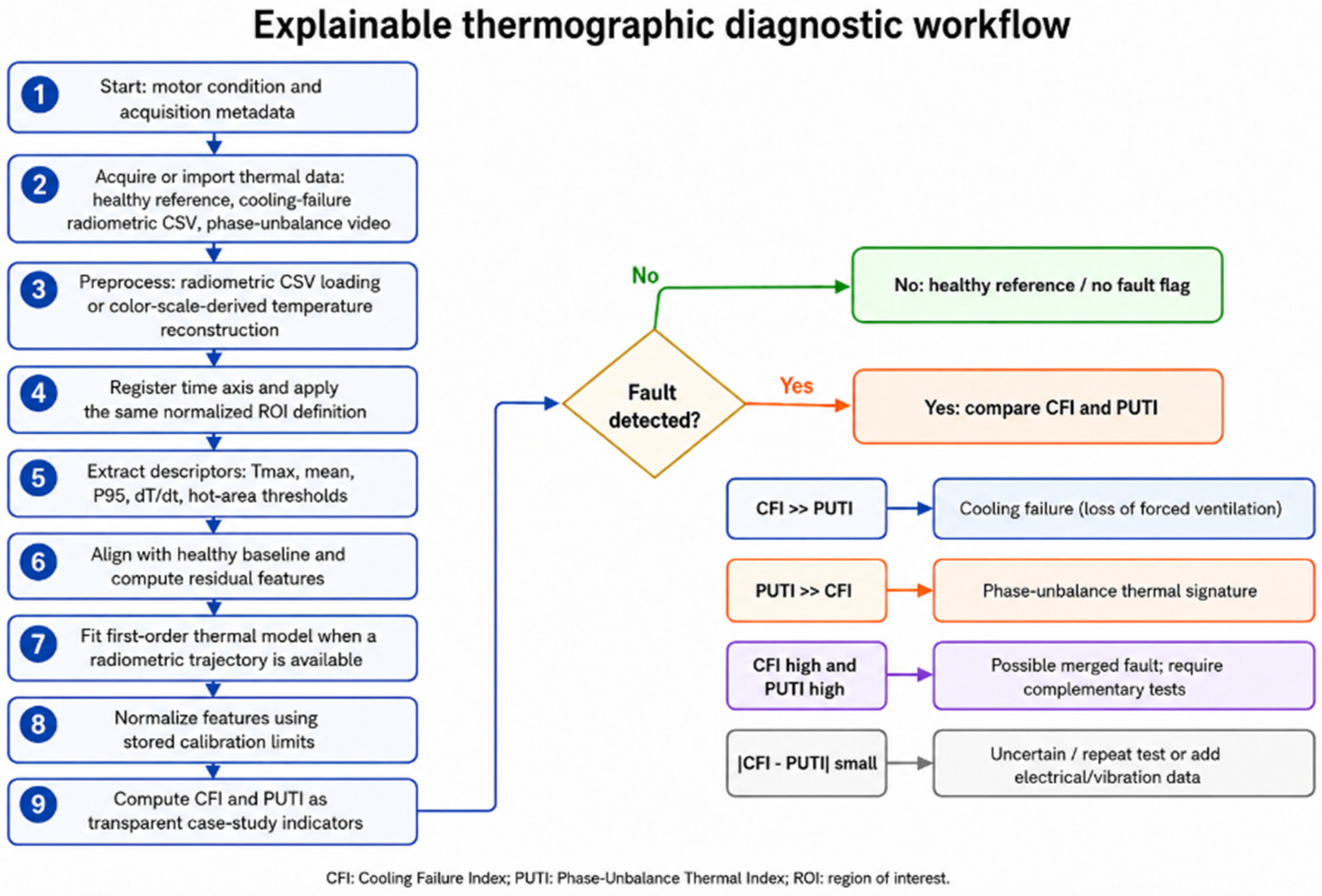
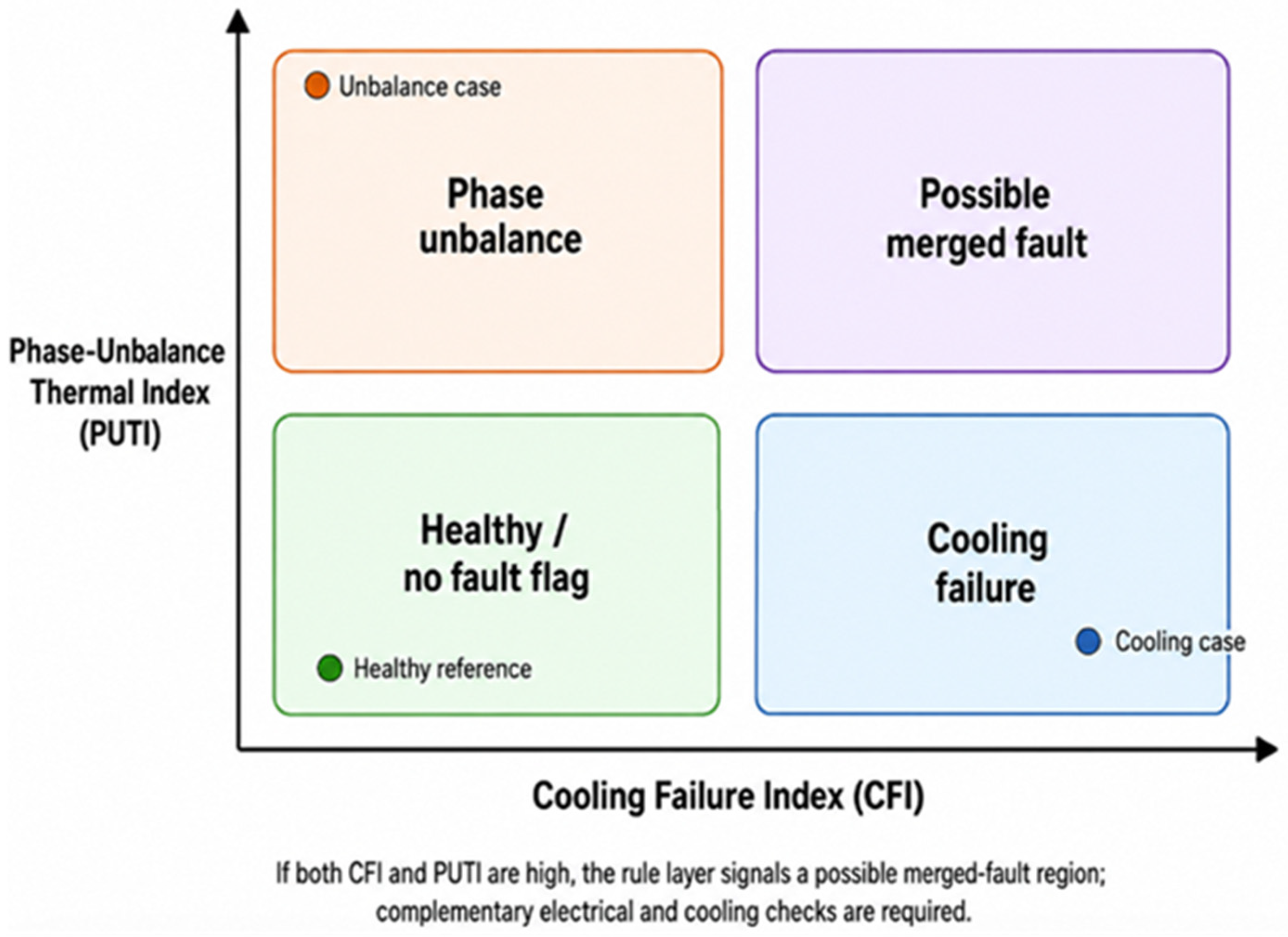
The complete algorithm is summarized in Figure 1. The workflow integrates thermographic input data from healthy operation, cooling failure radiometric images, and phase unbalance thermal video. After data preparation, ROI definition, and thermal feature extraction, the method compares each condition against the healthy thermal baseline through residual analysis. First-order thermal modeling and feature normalization are then used to compute CFI and PUTI. The final rule layer detects whether a fault is present and, only then, performs case-study-based discrimination between cooling failure and phase unbalance based on the dominant diagnostic index. If both indices are high, the result is treated as a possible merged-fault condition requiring complementary tests.

4. Experimental Setup

The experimental assessment was carried out on a three-phase squirrel-cage induction motor. The same motor was used under healthy operation and under the two analyzed faulty conditions in order to ensure that the observed thermal differences were associated with the imposed conditions and not with changes in machine geometry, rated characteristics, or thermal construction. The word “assessment” is used deliberately because the available dataset supports proof-of-concept evaluation, not full statistical validation of a universal classifier.

The tested motor was a Siemens 1LA2080-4AA10 induction motor rated at 1.1 kW and 1410 rpm. The motor was operated on the same laboratory bench for the healthy and faulty acquisitions, preserving the same mechanical coupling, camera position, acquisition rate, and ROI definitions. The rated characteristics of the machine are summarized in

Table 2. Rated characteristics of the tested induction motor.

Parameter	Value
Model	1LA2080-4AA10
Rated power, Pn	1.1 kW
Rated speed, nn	1410 rpm
Rated voltage, Un	400 V (Y)/230 V (Delta)
Rated current, In	2.7 A (Y)/4.6 A (Delta)
Rated power factor, cos phi	0.8
Number of rotor bars	28
Synchronous speed	1500 rpm
Nominal slip	6.00%
Mechanical frequency	23.50 Hz
Angular speed	147.65 rad/s
Rotor bar passing frequency	658.0 Hz

. The synchronous speed of 1500 rpm corresponds to a four-pole machine supplied at 50 Hz, while the rated mechanical speed of 1410 rpm gives a nominal slip of approximately 6%. The mechanical frequency in Table 2 is f_m = n/60 = 23.50 Hz, and the rotor-bar-passing frequency is f_RBPF = N_b f_m = 28 × 23.50 = 658.0 Hz. These frequencies are reported to document the motor, not because the 1 frame/s thermal acquisition is intended to sample electromechanical frequency content.

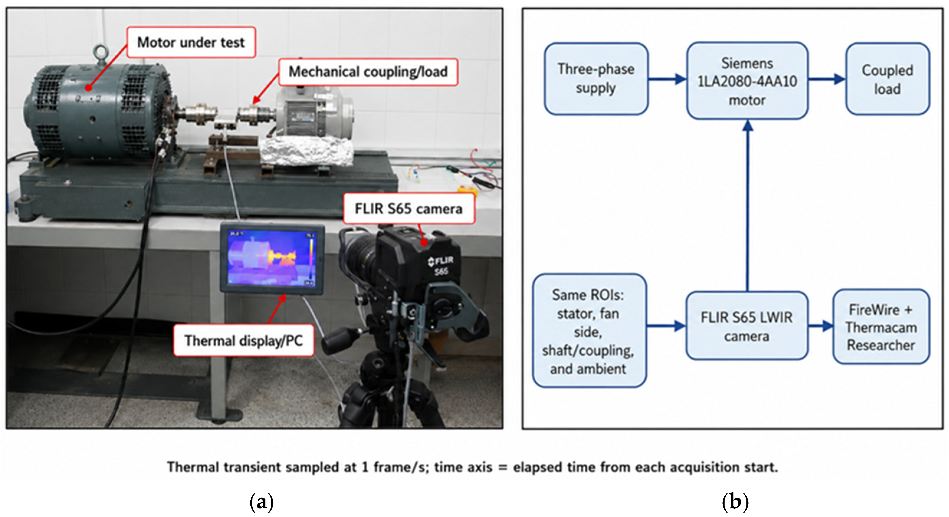
The thermal behavior of the motor was monitored using a long-wave infrared FLIR S65 thermal camera. The camera was connected to a portable computer through a FireWire interface and operated using Thermacam Researcher software v2.10. This software allowed real-time visualization and recording of the temperature distribution over the visible surface of the motor.

Thermographic data were acquired at a sampling rate of 1 frame/s. This acquisition rate is suitable for thermal transient analysis because the motor-frame temperature evolves much more slowly than electrical or mechanical variables. With fitted thermal time constants close to 28 min in the cooling failure case, the relevant thermal envelope is several orders of magnitude slower than 1 Hz. Therefore, the thermal sampling rate is adequate for temperature trajectories, hot area expansion, and ROI residuals, although it is not suitable for vibration, current, or rotor bar frequency analysis. The thermographic acquisition was maintained during the motor operation period until the thermal response approached stabilization. The experimental acquisition system is summarized in

Table 3. Thermographic acquisition setup and data sources.

Parameter	Value
Infrared camera	FLIR S65
Spectral band	LWIR
Interface	FireWire
Software	Thermacam Researcher
Thermographic sampling rate	1 frame/s
Image size	640 × 480 pixels
Fault classes considered	Healthy reference, cooling failure, phase unbalance condition (50% resistive bank setting)

, and Figure 2 shows the thermographic test bench.

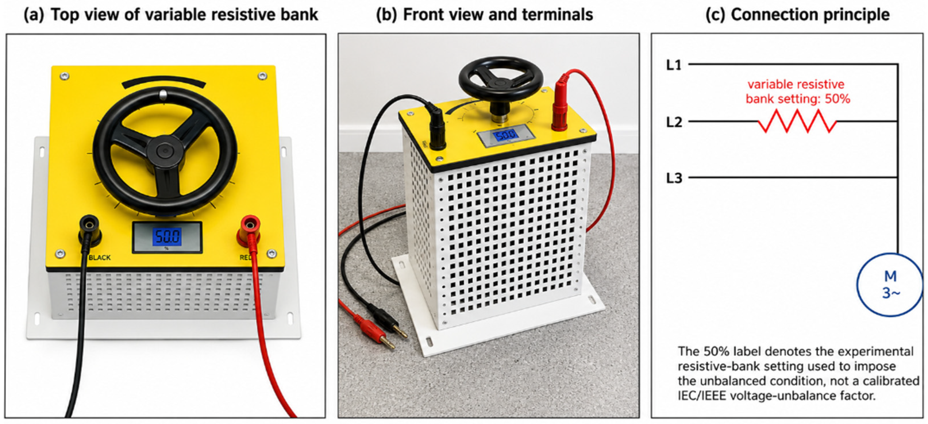
For the phase unbalance test, a variable resistive bank was used as part of the experimental bench to impose and adjust the unbalanced operating condition between phases. The device allowed the electrical asymmetry applied to one phase path to be established in a controlled laboratory environment, enabling the analysis of the corresponding transient thermal response. Figure 3 includes photographs of the resistive bank and a simplified connection diagram to clarify that the “50%” label corresponds to the bench setting of the resistive bank rather than to a calibrated VUF value.

For the phase unbalance condition, the exported thermal information was available as a color-mapped video sequence rather than as radiometric CSV matrices. Therefore, the temperature field was reconstructed from the visible thermal scale and used mainly for relative thermal trend analysis, ROI comparison, and interpretation of the stator-dominated thermal signature. The absolute temperature values obtained from this reconstruction are treated as estimates and are not used to claim the same metrological accuracy as the radiometric cooling failure data.

Analyzed Operating Conditions

Three thermal conditions were considered in the experimental study: healthy operation, cooling failure produced by loss of forced ventilation, and a phase unbalance condition imposed with the variable resistive bank. The healthy condition was used as the reference thermal behavior of the motor. The two faulty cases were selected because both can produce an increase in motor surface temperature but are caused by different physical mechanisms.

The cooling failure condition was produced by operating the motor without effective forced ventilation. This condition simulates a fan-related fault or severe degradation of the motor cooling system. Since the fan contributes to convective heat removal from the motor frame, its absence or malfunction is expected to produce a global increase in the thermal level of the machine and a progressive expansion of high-temperature regions.

The phase unbalance condition was produced by operating the motor with the variable resistive bank adjusted to the 50% setting. This value denotes the experimental setting of the unbalance-imposing device. It does not mean that all phases were dropped to 50%, nor does it represent a calibrated 50% voltage unbalance factor. Because the original post-processing package did not include synchronized phase voltage, phase current, power, speed, calibrated mechanical load, ambient temperature log, or warm-up records, the repeatability of this condition is explicitly limited and the results are interpreted as a qualitative thermal signature of an imposed phase unbalance scenario. This limitation is explicitly stated to avoid overinterpretation. In

Table 4. Experimental conditions analyzed in this work.

Condition	Description	Expected Thermal Behavior
Healthy operation	Motor operating without imposed fault	Reference transient and steady-state thermal behavior
Cooling failure	Motor operating without effective forced ventilation	Global overheating, hot area expansion, high final thermal level
Phase unbalance condition	Motor operating with resistive bank at the 50% setting	Moderate stator-dominated thermal increase; VUF not calibrated from synchronized electrical records

it is shown the conditions analyzed for the experiments.

Two types of thermographic data were used in the study. For the cooling failure condition, the thermal data were available as radiometric CSV files exported from the thermographic acquisition system. Each CSV file contains a two-dimensional thermal matrix in which each pixel corresponds to a temperature value. The available files correspond to different acquisition times between 40 min and 85 min of operation. Consequently, in the cooling failure analysis, time denotes the elapsed operating time in minutes from motor start. However, the analyzed interval begins at 40 min because only the CSV files exported from that point onward were available for processing.

For the phase unbalance condition, the thermal data were available as a color-mapped thermographic video. Since the exported video does not contain direct radiometric values for each pixel, an approximate temperature reconstruction was performed using the visible thermal color scale. The reconstructed sequence was used to analyze the relative thermal evolution and the stator-dominated thermal signature associated with the imposed phase unbalance condition. In this analysis, time is expressed in seconds from the first reconstructed video frame. Therefore, this time reference represents the duration of the reconstructed video sequence and should not be directly compared with the elapsed operating time, expressed in minutes from motor start, used in the cooling failure analysis.

The experimental setup therefore combines a controlled laboratory induction motor test bench with infrared thermographic monitoring. The same Siemens 1LA2080-4AA10 motor, bench configuration, camera position, and ROI definitions were used for healthy operation, cooling failure, and phase unbalance. Nevertheless, the available documentation does not allow a full load and electrical state equivalence analysis across all conditions. The present results are therefore reported as a proof-of-concept case study and not as a metrologically complete load-sweep validation.

5. Results

This section presents the results obtained with the proposed explainable thermographic fault diagnosis workflow. The analysis focuses on the healthy reference and two faulty operating conditions imposed on the same three-phase squirrel-cage induction motor: cooling failure and a resistive-bank-induced phase unbalance condition. The objective is to determine whether transient thermal signatures can provide interpretable evidence for separating a cooling-related fault from an electrical-supply-related fault in this specific case study.

The two fault cases were processed using the same general pipeline: data preparation, region-of-interest (ROI) definition, extraction of thermal descriptors, transient analysis, first-order thermal modeling where appropriate, calculation of diagnostic indices, and rule-based, case-study-based discrimination. However, the quantitative strength of the evidence differs between the two datasets: cooling failure is supported by radiometric CSV matrices, whereas phase unbalance is supported by an estimated color-scale-derived thermal sequence.

All numerical values reported in this section correspond to the ROI definitions used in the final processing pipeline. The global quantities refer to the complete analyzed thermal scene, whereas ROI quantities refer to physically meaningful zones of the motor, including the stator region, fan-side region, shaft/coupling region, and ambient reference region. The healthy reference is reported only as the zero-residual reference condition used by the fault detection rule, not as an independently repeated healthy test; because the raw healthy CSV/video trajectory was not available as a separate export in the manuscript package, no additional fabricated healthy heating curve is introduced.

Table 5. Compact summary of the analyzed conditions.

Condition	Data Source	Time Span	Stator Mean (Initial to Final, °C)	Global Max. (Initial to Final, °C)
Healthy reference	Motor-specific baseline	Reference trajectory	Residuals = 0 by definition	Fault flag = False
Cooling failure	Radiometric CSVs	40–85 min	59.48 to 69.77	77.20 to 91.60
Phase unbalance condition	MP4 colorbar-derived sequence	0–675 s	24.81 to 40.35	32.96 to 43.38

summarizes the analyzed conditions.

The results show that both faults increased the motor temperature but with different thermal manifestations. The cooling failure condition produced a severe and global thermal rise, accompanied by a strong increase in the area above 80 °C. By contrast, the phase unbalance condition produced a more localized stator-dominated increase without severe hot area expansion above 80 °C. These observations are used for case-study-based discrimination, not for claiming universal diagnostic accuracy.

5.1. Radiometric Thermal Response Under Cooling Failure

The cooling failure condition was evaluated using radiometric thermal images exported at 40, 45, 50, 55, 60, 65, 70, 75, 80, and 85 min of operation. Since these files contain direct pixel-wise temperature values, they allow quantitative evaluation of the thermal field and its evolution under degraded heat evacuation. The time axis in this subsection corresponds to elapsed operating time in minutes; the first available CSV frame is at 40 min, so the plotted interval does not represent the complete heating history from a cold start.

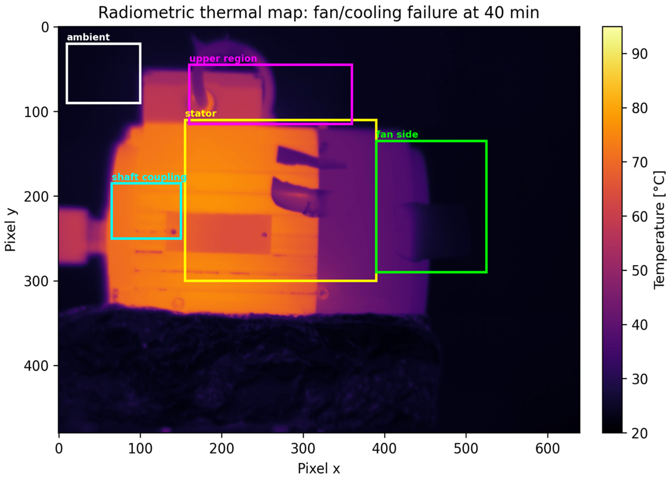
Figure 4 shows the radiometric thermal map at 40 min. At this time, the motor already exhibited a clear thermal elevation, but the highest temperature region had not yet expanded to the most severe levels observed later in the test. The stator and shaft/coupling regions were hotter than the fan-side and ambient regions, indicating that the main heat accumulation was associated with the motor body and the mechanically connected region.

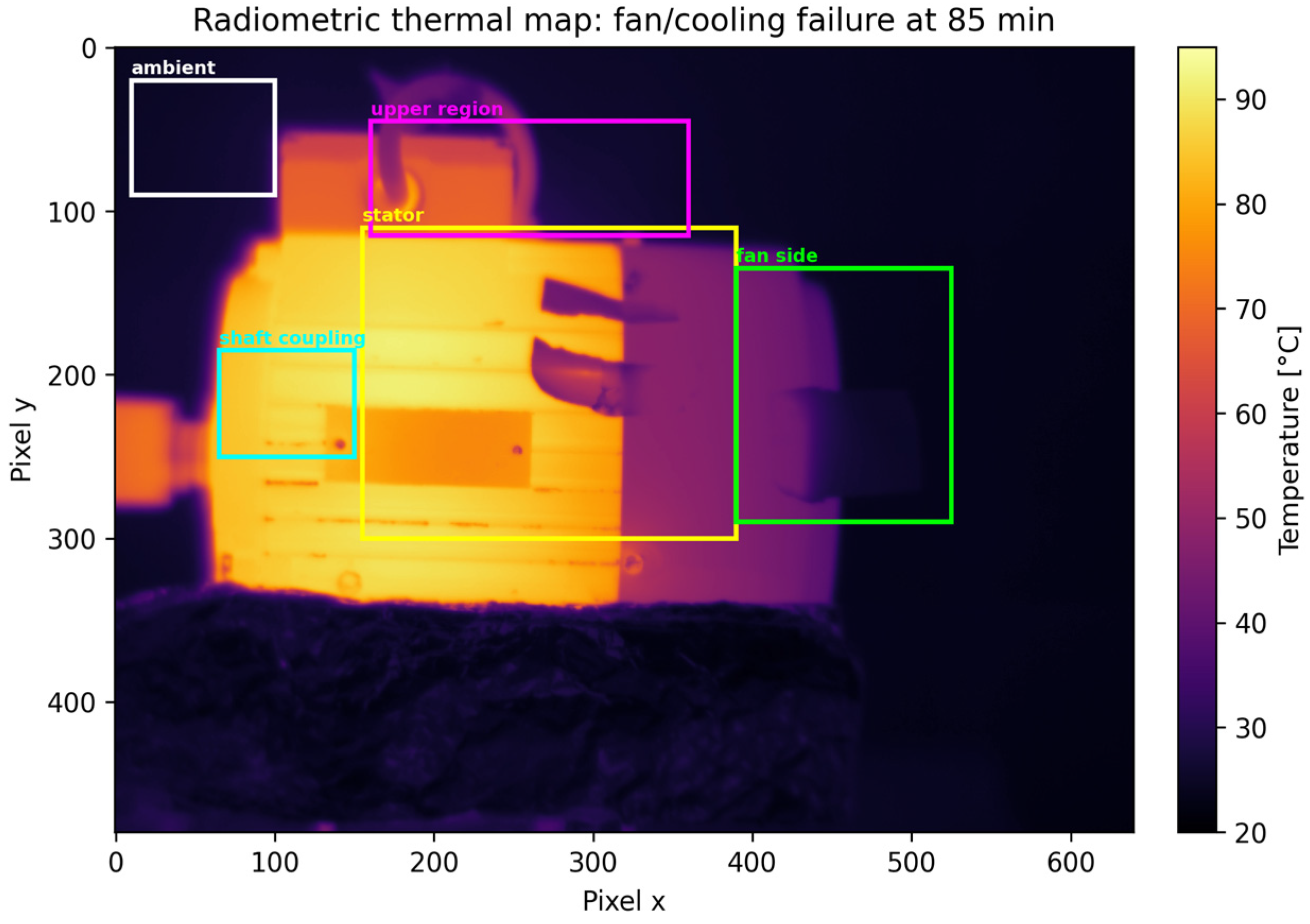
Figure 5 shows the same condition at 85 min. The thermal field was significantly more severe. The maximum temperature increased to 91.6 °C, and the hot region expanded across a larger portion of the visible motor surface. This behavior is consistent with a loss of forced convection because the heat generated inside the motor was not removed efficiently and progressively accumulated in the motor frame and adjacent regions.

Table 6. Radiometric thermal descriptors under cooling failure.

Time (min)	Global Max. (°C)	Stator Mean (°C)	Stator P95 (°C)	ΔT Stator–Ambient (°C)	Area > 80 °C (px)
40	77.2	59.48	76.0	35.08	0
45	80.1	61.55	78.9	36.93	8
50	82.7	63.34	81.4	38.39	7696
55	84.6	64.69	83.4	39.56	21,815
60	86.3	65.89	85.0	40.59	30,169
65	87.8	67.03	86.4	41.49	36,001
70	89.0	67.97	87.6	42.15	38,788
75	89.9	68.44	88.5	42.68	40,429
80	90.8	69.13	89.3	43.22	42,019
85	91.6	69.77	90.1	43.69	43,399

summarizes the evolution of the most relevant radiometric descriptors for the cooling failure test. The global maximum temperature increased from 77.2 °C at 40 min to 91.6 °C at 85 min, corresponding to a rise of 14.4 °C. The stator mean temperature increased from 59.48 °C to 69.77 °C, and the area above 80 °C expanded from 0 to 43,399 pixels. These descriptors quantify both thermal severity and spatial expansion, which were expected given that forced convection was degraded.

The results in Table 6 show three important aspects. First, the maximum temperature and stator high-temperature descriptors increased monotonically during the analyzed interval, indicating progressive thermal severity. Second, the stator-to-ambient temperature difference increased from 35.08 °C to 43.69 °C, confirming that the motor body deviated increasingly from the thermal background. Third, the stator-to-fan-side difference increased from 30.10 °C to 37.54 °C, indicating that the stator region became progressively hotter than the fan-side region. This behavior is consistent with reduced heat evacuation and accumulation of heat in the main motor body.

5.2. Thermal Evolution and Hot Area Expansion Under Cooling Failure

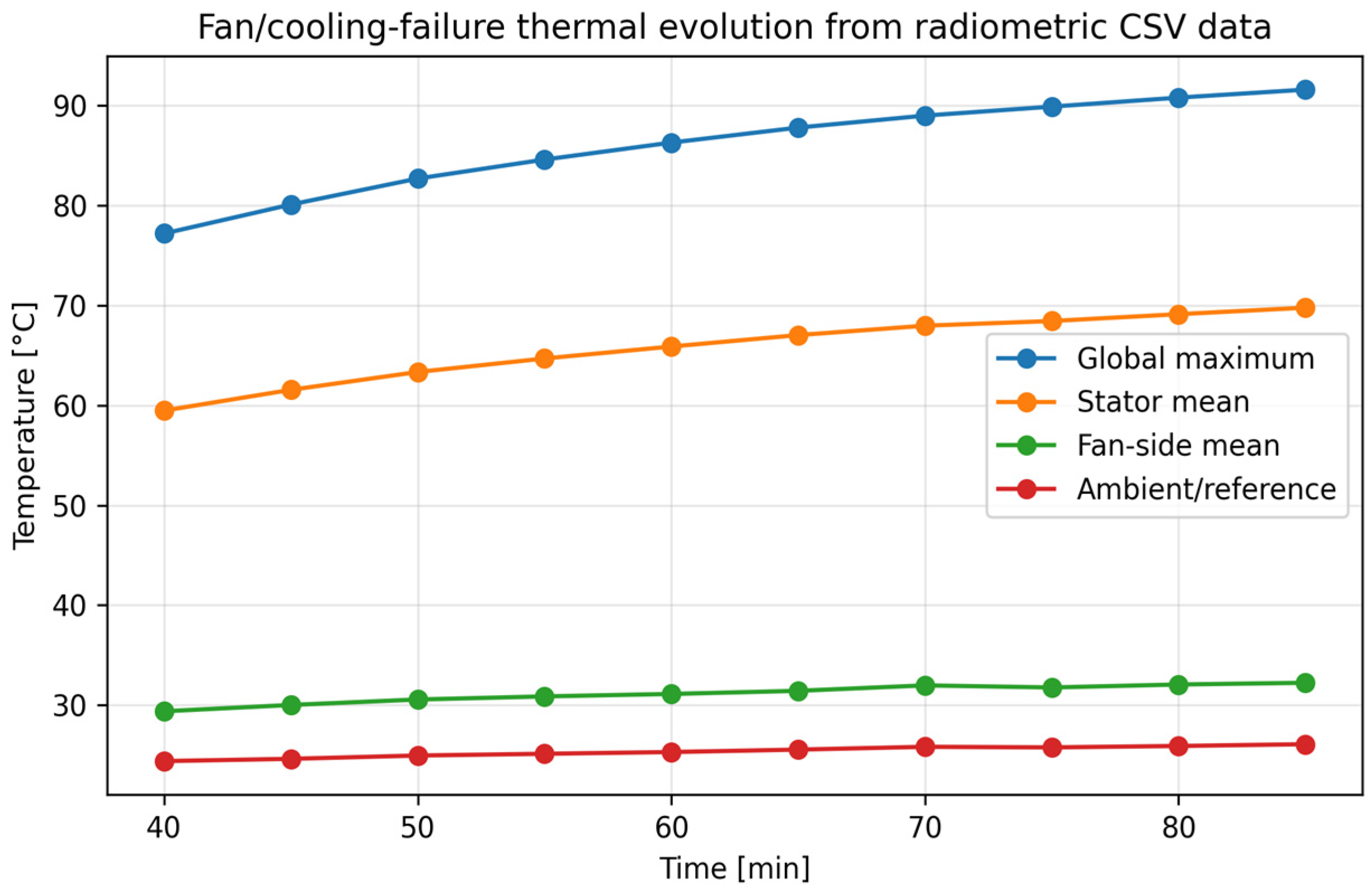
Figure 6 presents the temporal evolution of representative global and ROI-based temperature descriptors for the cooling failure condition. The global maximum temperature and the stator-related descriptors showed sustained upward trends over the complete analyzed CSV interval. This time vector is expressed in minutes of motor operation and differs from the second-based time vector used for the reconstructed phase unbalance video.

The global maximum temperature increased by 14.4 °C, while the stator mean temperature increased by 10.30 °C. The difference between the stator and the ambient ROI increased by 8.61 °C, and the difference between the stator and the fan-side ROI increased by 7.45 °C. These values indicate that the thermal rise represents not only an absolute increase in temperature but also a differential deviation between the stator region and other reference zones.

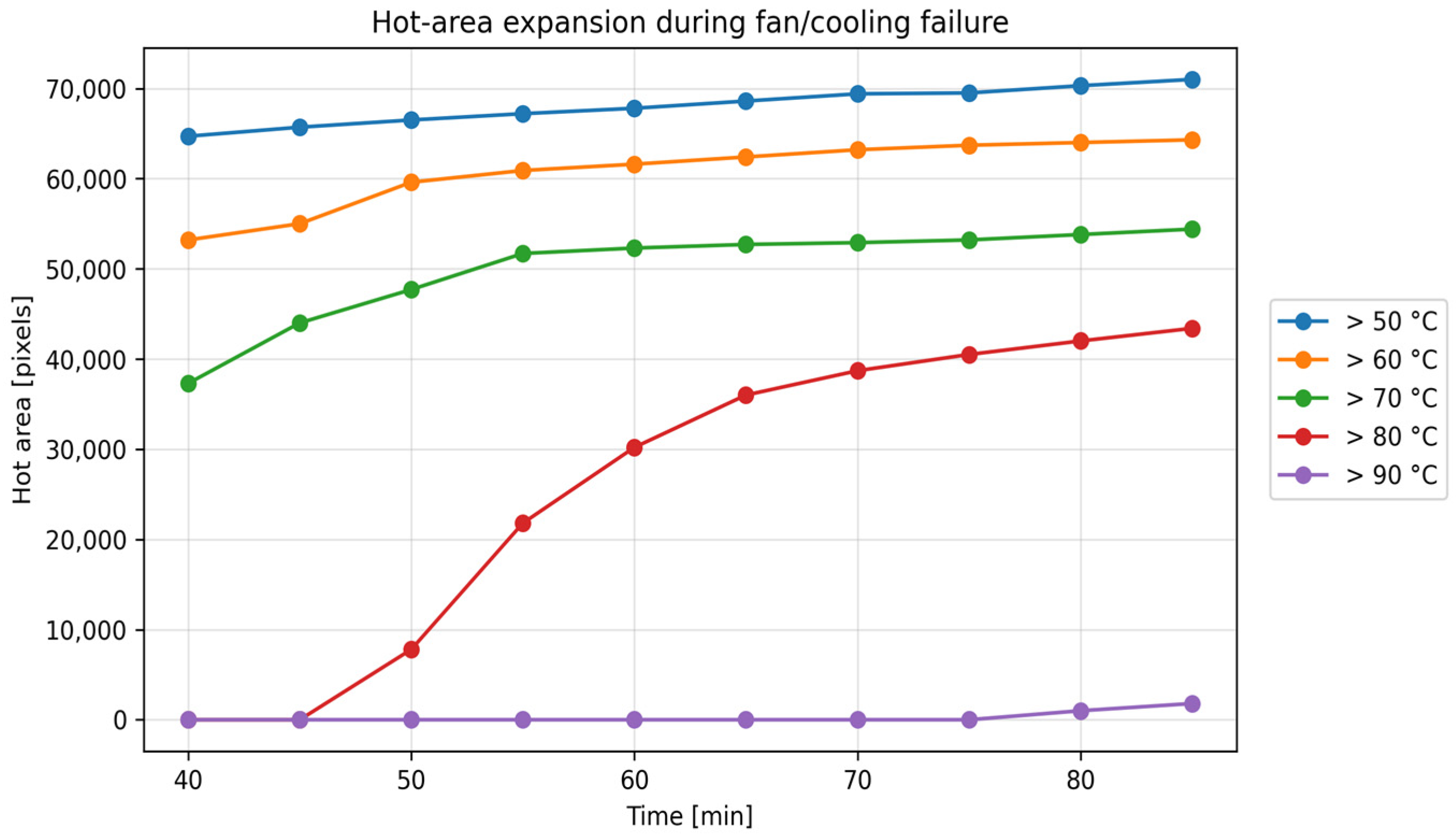
Figure 7 shows the evolution of the number of pixels above selected thermal thresholds. This feature is particularly relevant for cooling failure diagnosis because it measures the spatial expansion of abnormal heating. The area above 40 °C increased from 83,584 pixels to 97,615 pixels, and the area above 50 °C increased from 64,741 pixels to 70,960 pixels. More importantly, the area above 80 °C increased from 0 pixels at 40 min to 43,399 pixels at 85 min. The apparently abrupt behavior at the 80 °C threshold is expected in thresholded area curves: once a contiguous region crosses the threshold, many neighboring pixels are counted simultaneously. It therefore reflects crossing of a severe heating threshold rather than an independent oscillatory thermal phenomenon.

The sharp increase in the number of pixels above 80 °C is one of the clearest thermal indicators of cooling degradation in this dataset. Unlike the maximum temperature, which can be influenced by a small local hot spot, the hot area descriptor reflects how much of the motor surface is affected by severe heating. The thresholded areas are nevertheless sensitive to camera calibration, emissivity, segmentation, and radiometric accuracy; therefore, their direct quantitative use should be restricted to comparable acquisition conditions.

5.3. First-Order Thermal Modeling of Cooling Failure

The radiometric thermal trajectories were fitted using a first-order thermal model to obtain compact descriptors of the transient heating process. The fit was performed on the available CSV points between 40 and 85 min of operation. Time was expressed relative to the first analyzed frame for numerical fitting, while the

Table 7. First-order thermal model parameters for the cooling-failure condition.

Variable	Estimated T∞ (°C)	$\mathit{\tau }$ (s)	$\mathit{\tau }$ (min)	R2	Mean Heating Rate (°C/min)
Global maximum temperature	95.13	1681.55	28.03	0.9998	0.3200
Stator mean temperature	72.38	1720.90	28.68	0.9995	0.2289
Fan-side mean temperature	32.79	1541.45	25.69	0.9863	0.0634

reports the corresponding time constants in both seconds and minutes.

$$T\left(t\right)=T_{\mathrm{\infty }}-\left(T_{\mathrm{\infty }}-T_0\right)\mathrm{e}\mathrm{x}\mathrm{p}\left(-t/\tau \right),$$

(47)

where T∞ is the estimated asymptotic temperature and τ is the thermal time constant. Table 7 reports the fitted parameters for the global maximum temperature, stator mean temperature, and fan-side mean temperature. These parameters are valid only for the analyzed operating interval and should not be extrapolated to different load levels or cooling configurations without new calibration.

The global maximum temperature model estimated an asymptotic temperature of 95.13 °C and a thermal time constant of 28.03 min, with an excellent coefficient of determination (R² = 0.9998). The stator mean temperature showed a similar time constant of 28.68 min and an estimated asymptotic value of 72.38 °C, consistent with Table 7. The fan-side mean temperature showed a much lower asymptotic value of 32.79 °C, indicating that the thermal anomaly was not uniformly expressed in all visible regions.

These model parameters support the physical interpretation of cooling failure. The high asymptotic maximum temperature and the strong hot area expansion indicate that the degraded cooling condition drives the motor toward a high-temperature operating regime. The comparable time constants of the global maximum and stator mean responses suggest a coherent heating process over the motor body rather than an isolated short-duration thermal anomaly.

5.4. Color-Scale-Derived Thermal Response Under the Phase Unbalance Condition

The phase unbalance condition was analyzed using the exported thermal video obtained with the resistive bank at the 50% setting. Since the MP4 file does not provide direct radiometric pixel values, temperature reconstruction was performed using the visible thermal color scale. As a result, the values reported in this subsection are estimated temperatures and should be interpreted as thermal trend descriptors rather than as fully calibrated radiometric measurements.

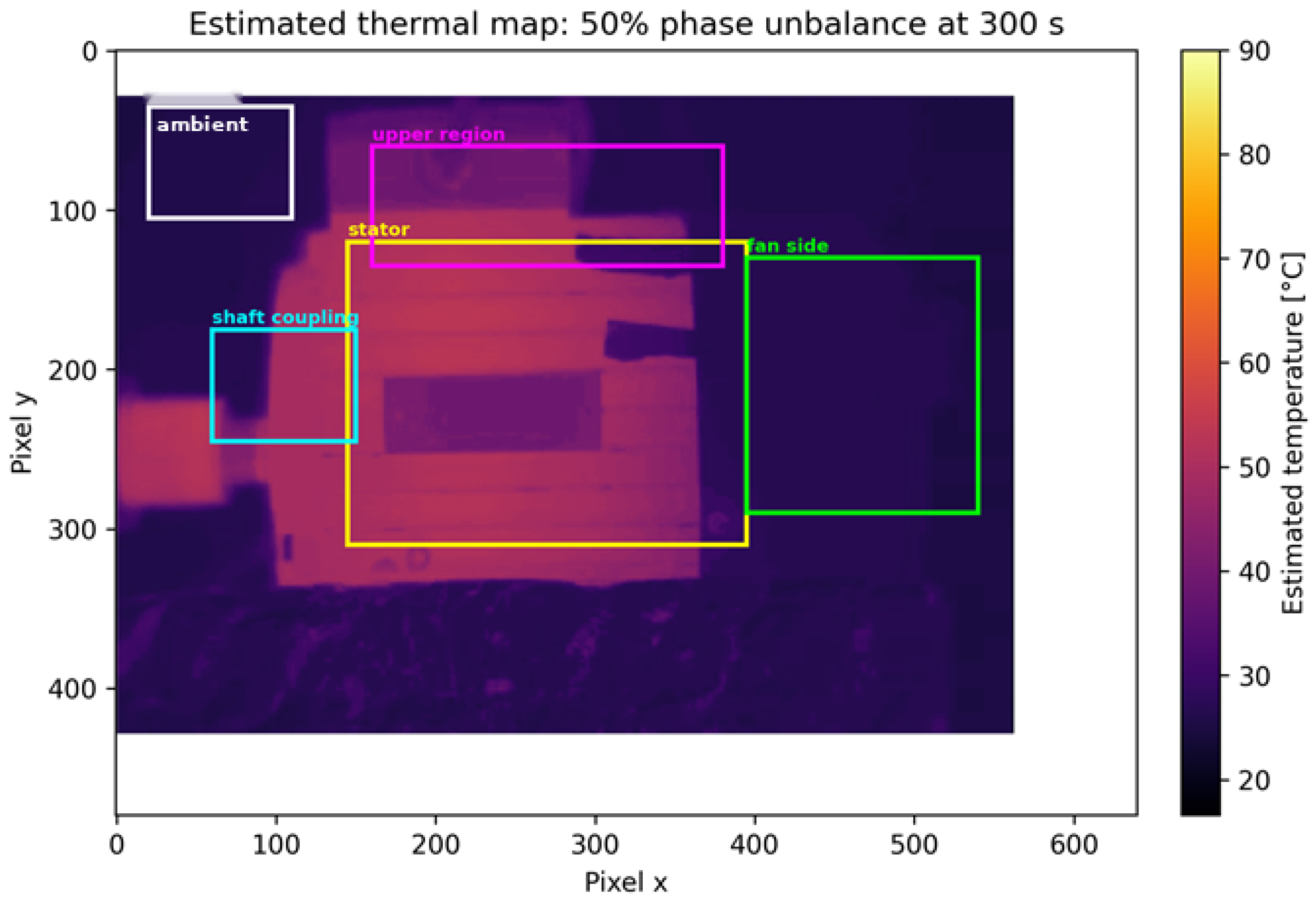
Figure 8 shows the estimated thermal map at 300 s from the first reconstructed video frame. The reconstructed temperature field indicated a clear thermal rise in the stator region. However, the phase unbalance thermal pattern was less severe than the cooling failure case. In particular, the reconstructed sequence did not show an area above 80 °C, reinforcing the interpretation of a localized stator-dominated signature rather than global overheating.

Table 8. Selected color-scale-derived thermal descriptors under the phase unbalance condition.

Time (s)	Global Max. (°C)	Stator Mean (°C)	Fan-Side Mean (°C)	ΔT Stator–Fan (°C)	Area > 50 °C (px)	Area > 80 °C (px)
0	32.96	24.81	25.06	-0.25	0	0
60	45.43	37.81	25.70	12.11	0	0
120	49.93	41.98	26.36	15.62	0	0
180	51.97	43.18	26.14	17.04	5317	0
240	53.20	43.98	26.43	17.55	16,037	0
300	53.40	44.26	26.52	17.74	21,765	0
450	53.61	44.13	26.58	17.54	20,435	0
600	47.88	44.68	31.74	12.95	0	0
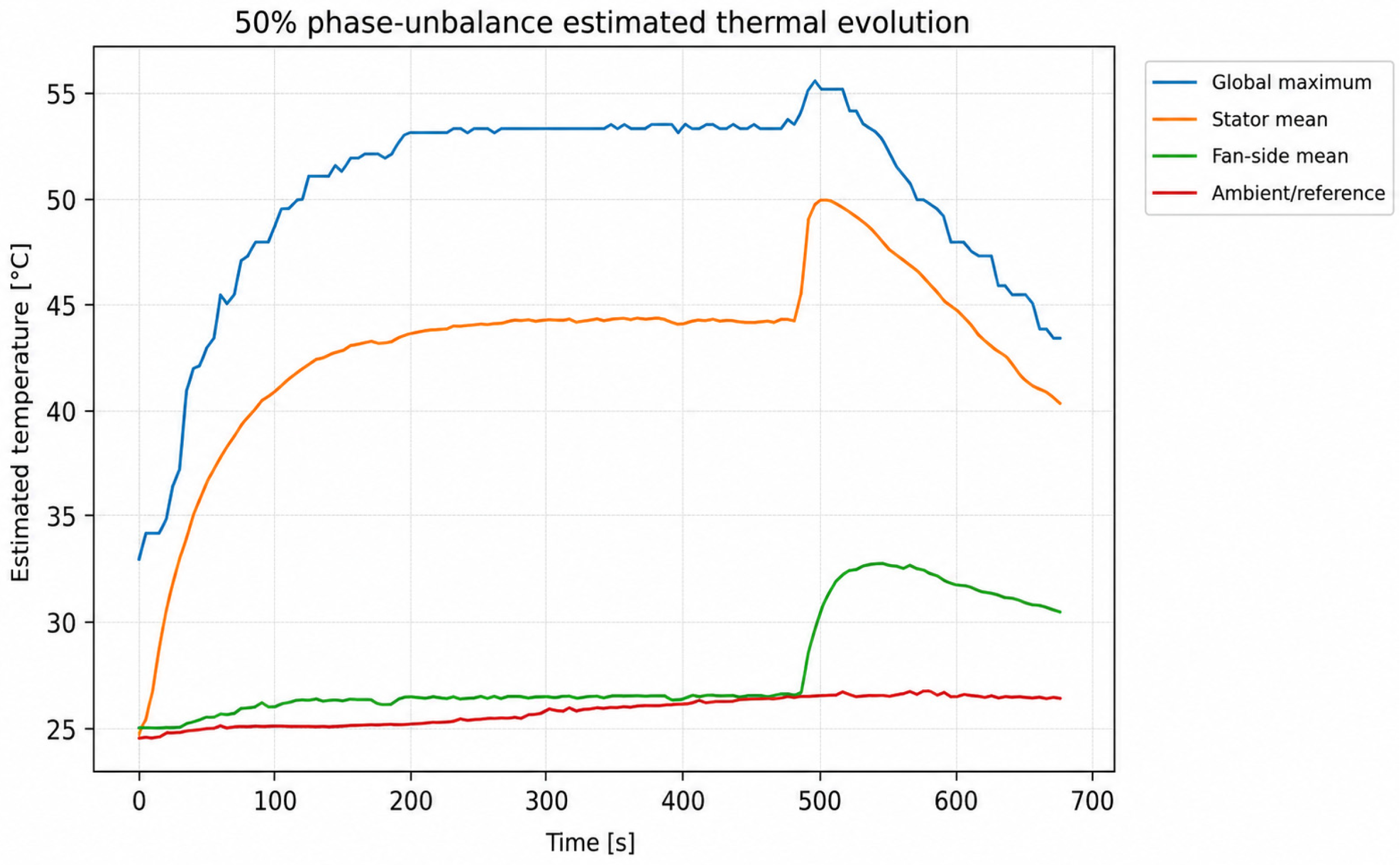
675	43.38	40.35	30.52	9.83	0	0

summarizes selected time instants from the reconstructed phase unbalance sequence. The stator mean temperature increased from 24.81 °C at the beginning of the sequence to 40.35 °C at the final analyzed time, corresponding to a final increase of 15.54 °C. The stator mean temperature reached its maximum value of approximately 49.94 °C around 500 s. The maximum global temperature reached approximately 55.65 °C around 495 s, and then decreased.

The phase unbalance sequence showed a rapid initial increase in the stator ROI. At 60 s, the stator mean temperature had already increased to 37.81 °C, and the stator-to-fan-side difference reached 12.11 °C. Around 240–300 s, the stator temperature was approximately 44 °C, with a stator-to-fan-side difference between 17.55 °C and 17.74 °C. This confirms that the thermal signature was dominated by the stator region.

5.5. Transient Evolution Under the Phase Unbalance Condition

Figure 9 presents the estimated temporal evolution of the main temperature descriptors under the phase unbalance condition. The time axis is expressed in seconds from the first reconstructed frame, not in minutes from motor start. The stator ROI showed the most relevant increase, whereas the ambient ROI remained comparatively stable. This behavior is consistent with an electrical loss mechanism that mainly affects the stator region.

The stator mean temperature increased by 15.54 °C between the first and final analyzed frames. However, the peak stator mean temperature reached approximately 49.94 °C around 500 s, corresponding to a maximum stator rise of approximately 25.13 °C with respect to the initial stator mean. The final stator-to-ambient difference was 13.90 °C, while the final stator-to-fan-side difference was 9.83 °C. The maximum stator-to-fan-side difference reached approximately 20.46 °C around 490 s.

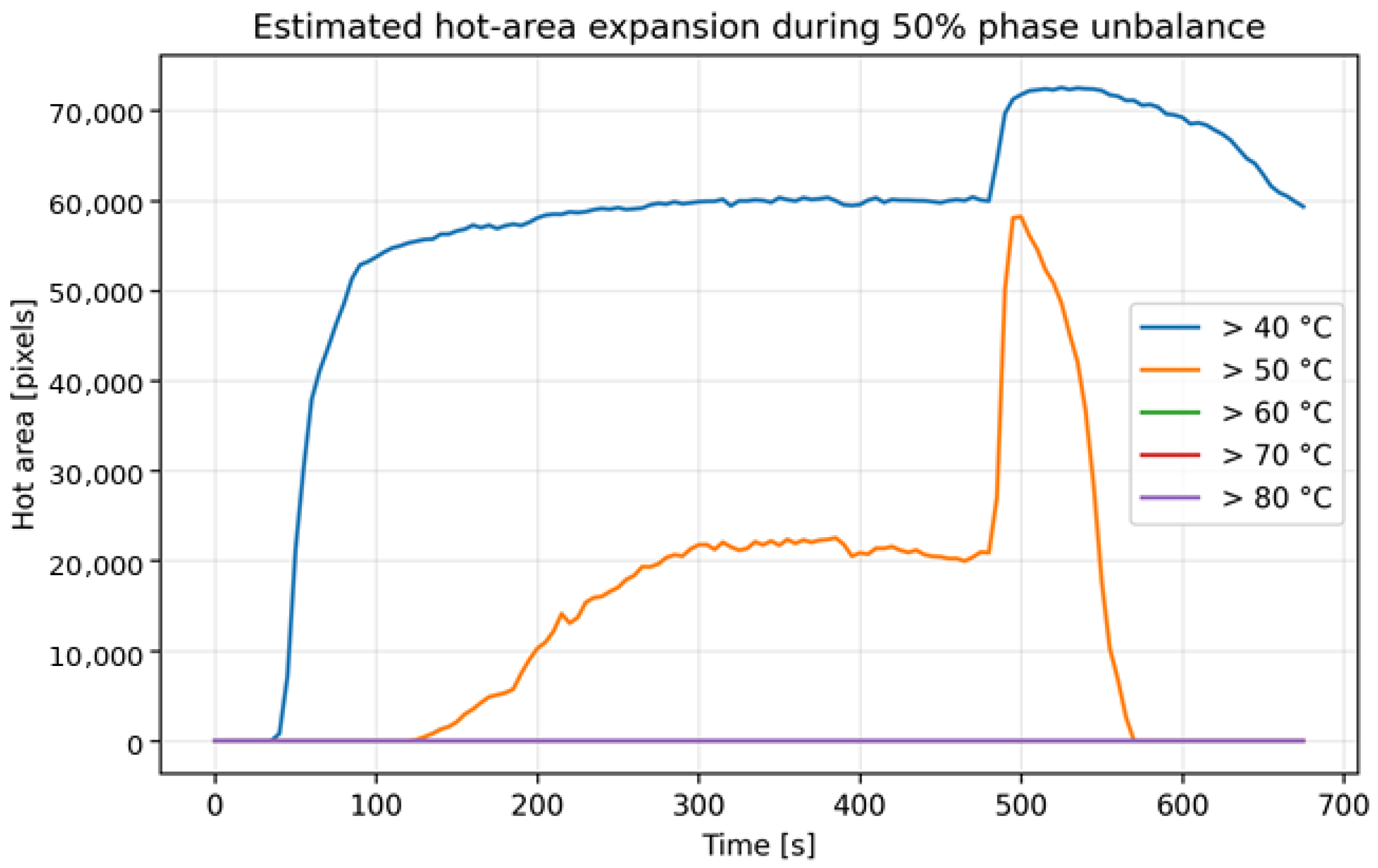
Figure 10 shows the estimated hot area evolution under phase unbalance. The reconstructed sequence showed a considerable number of pixels above 40 °C and a transient number of pixels above 50 °C. However, the area above 80 °C remained zero throughout the analyzed sequence. This is a key discriminating feature with respect to cooling failure, where severe hot area expansion above 80 °C was observed. The nonmonotonic behavior at lower thresholds is attributed to color scale reconstruction, palette quantization, and the changing visible thermal scene and should not be overinterpreted as a calibrated thermal oscillation.

The absence of pixels above 80 °C in the phase unbalance sequence indicated that this fault did not generate the severe global overheating observed in the cooling failure condition. Instead, the thermal response was characterized by a stator-dominated increase and moderate spatial spread. This supports the diagnostic assumption that phase unbalance and cooling failure can be separated using combined ROI-based and hot area descriptors.

5.6. Comparative Analysis of the Two Fault Signatures

The two faulty conditions produced different thermal responses despite both increasing the motor temperature. The cooling failure condition was characterized by high maximum temperature, strong stator-to-ambient deviation, and severe hot area expansion. The phase unbalance condition was characterized by a lower estimated maximum temperature, a stator-dominated rise, and no estimated area above 80 °C. Because the two data sources had different metrological quality, the comparison emphasizes signature morphology and diagnostic interpretation rather than strict numerical equivalence. In

Table 9. Comparative summary of the fault signatures.

Descriptor	Cooling Failure	Phase Unbalance Condition
Final global maximum	91.60 °C	43.38 °C
Maximum global temperature observed	91.60 °C	55.65 °C
Final stator mean	69.77 °C	40.35 °C
Final stator temperature rise	+10.30 °C	+15.54 °C
Final stator-to-ambient difference	43.69 °C	13.90 °C
Final stator-to-fan-side difference	37.54 °C	9.83 °C
Area above 80 °C	43,399 px	0 px
Main signature	Global overheating and hot area growth	Moderate stator-dominated thermal rise

it is showed a summary of the fault signatures.

The key differentiating feature is the combination of thermal severity and spatial expansion. The cooling failure case reached temperatures above 90 °C and produced a large area above 80 °C. This behavior is consistent with degraded heat evacuation. Conversely, the phase unbalance case produced a stator-dominated rise without any area above 80 °C. This suggests that the thermal anomaly was associated with additional electrical losses rather than a severe loss of cooling capability.

5.7. Explainable Diagnostic Indices

The extracted features were summarized using two physically interpretable diagnostic indices: the Cooling Failure Index (CFI) and the Phase Unbalance Thermal Index (PUTI). CFI was designed to respond to global overheating, high-temperature area expansion, stator-to-ambient deviation, and high asymptotic thermal level. PUTI was designed to respond to stator-dominated thermal deviation, stator-to-fan-side gradient, and limited severe hot area expansion. Both indices are preliminary author-defined indicators and are not established diagnostic standards.

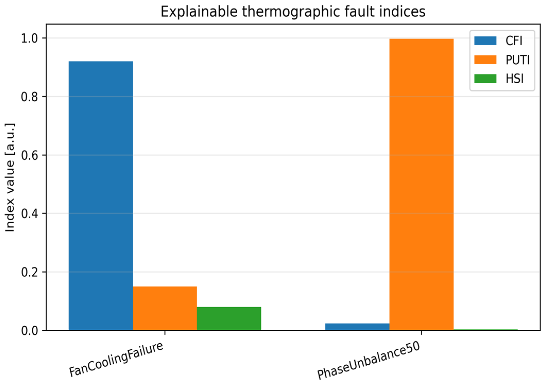
Figure 11 shows the values of the explainable indices for the two available fault classes. The cooling failure condition produced a high CFI value and a low PUTI value, whereas the phase unbalance condition produced a high PUTI value and a low CFI value. This behavior is consistent with the intended physical meaning of the indices. However, the result should be interpreted as proof-of-concept case-study-based separation because only two faulty cases and one healthy reference are available.

The rule-based decisions are summarized in

Table 10. Diagnostic indices and rule-based case-study-based decisions, including the healthy reference.

Condition	Fault Detected	Predicted Class	CFI	PUTI	Healthy Similarity Index (HSI)
Healthy reference	False	Healthy/no fault	0.0000	0.0000	1.0000
Cooling failure	True	Cooling failure	0.9193	0.1500	0.0807
Phase unbalance condition	True	Phase unbalance condition	0.0243	0.9971	0.0029

, which includes the healthy reference as a baseline consistency check. For the healthy baseline self-reference check, the residual-based fault flag is false and both CFI and PUTI are reported as zero-valued reference indicators. Cooling failure produced a CFI of 0.9193 and a PUTI of 0.1500. The rule layer therefore assigned the condition to the cooling failure class. The phase unbalance condition produced a CFI of 0.0243 and a PUTI of 0.9971. The rule layer therefore assigned the condition to the phase unbalance class. These decisions are not statistical performance metrics; they are transparent interpretations of the two analyzed cases.

The diagnostic rationale is physically interpretable. In the cooling failure case, the main evidence was the large increase in global maximum temperature, which reached 91.60 °C, and the expansion of the area above 80 °C to 43,399 pixels. In the phase unbalance case, the main evidence was the 15.54 °C increase in stator mean temperature and the final stator/fan-side gradient, together with the absence of severe high-temperature area expansion.

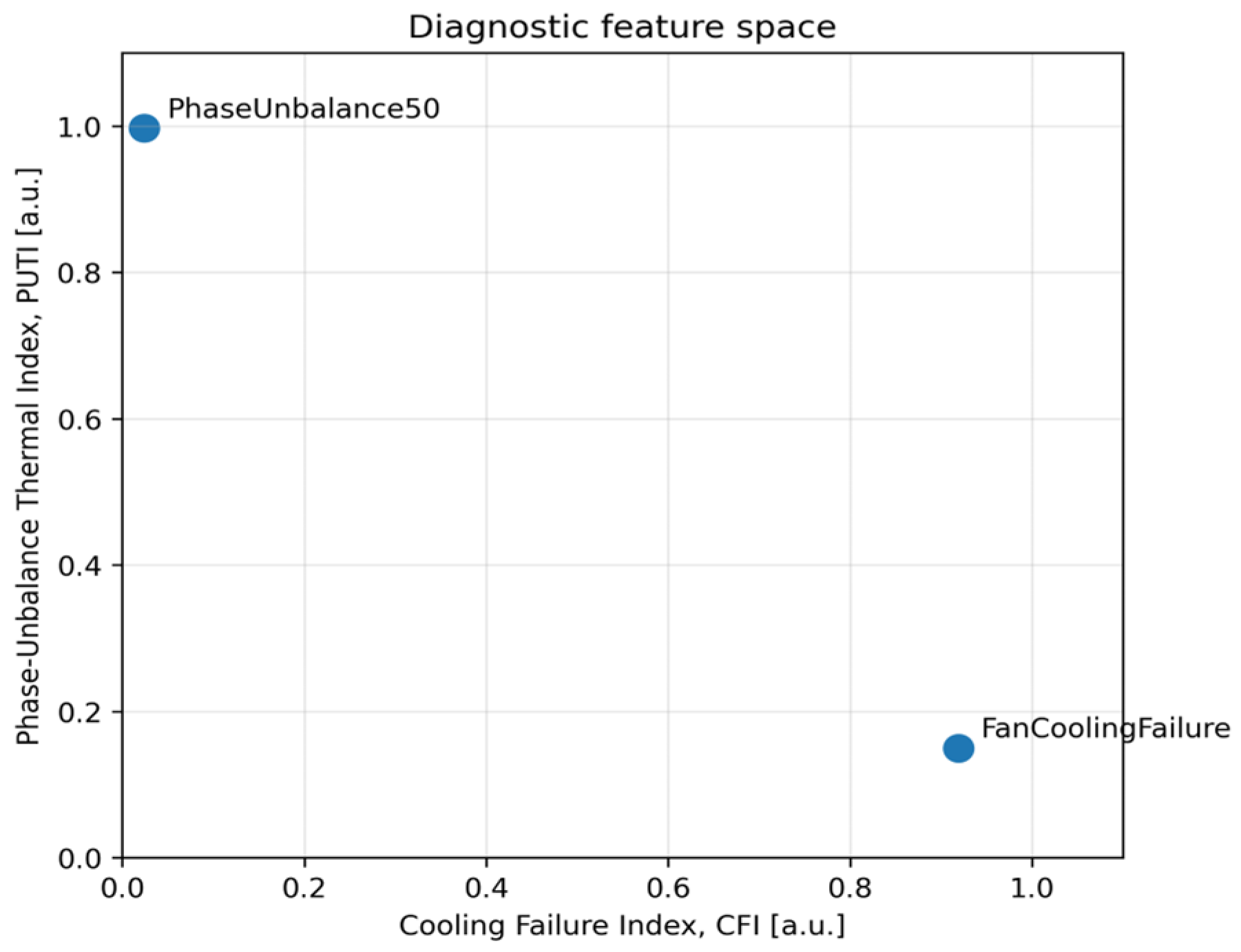
Figure 12 shows the two-dimensional diagnostic feature space defined by CFI and PUTI. The two fault classes appear in separated regions of the feature space. Although only two fault conditions are available in the present case study, the separation indicates that the selected indices encode different physical evidence: severe global overheating for cooling failure and stator-dominated thermal deviation for phase unbalance. The figure should not be interpreted as proof of general classification performance.

5.8. Rule-Based Fault Detection and Discrimination

The final rule layer performs two tasks: fault detection and fault discrimination. A fault is detected when the thermal response deviates from the expected healthy behavior according to residual-based indicators. Only after a fault is detected is the condition assigned to the dominant case study class by comparing CFI and PUTI. This sequence avoids forcing the healthy reference into a fault class.

For the cooling failure condition, CFI was much larger than PUTI. Therefore, the decision rule

$$\mathrm{C}\mathrm{F}\mathrm{I}>\mathrm{P}\mathrm{U}\mathrm{T}\mathrm{I}$$

(48)

is assigned the condition to the cooling failure class. The underlying explanation is that the fault produced severe global overheating and high-temperature area expansion, which are the expected consequences of degraded forced convection.

For the phase unbalance condition imposed with the 50% resistive bank setting, the PUTI value was much larger than the CFI value. Therefore, the decision rule

$$\mathrm{P}\mathrm{U}\mathrm{T}\mathrm{I}>\mathrm{C}\mathrm{F}\mathrm{I}$$

(49)

is assigned the condition to the phase unbalance class. The underlying explanation is that the fault produced a stator-dominated thermal deviation without the large area above 80 °C observed under cooling failure.

The rule-based diagnostic structure is especially useful for interpretability. Rather than returning only a class label, the method explains the diagnostic decision through physical descriptors: maximum temperature, hot area expansion, stator residual, stator-to-ambient deviation, and stator-to-fan-side deviation.

6. Discussion

The results support the feasibility of explainable, ROI-based thermographic discrimination between cooling failure and a phase unbalance thermal signature in the tested three-phase induction motor. The proposed workflow does not rely only on visual inspection or maximum temperature values but instead combines transient thermal evolution, spatial expansion, healthy baseline residuals, and fault-oriented indices. The term discrimination is used here in a case study sense and does not imply validated classifier performance.

The first relevant finding is that the cooling failure condition produced severe global overheating. The maximum radiometric temperature increased from 77.2 °C to 91.6 °C, while the area above 80 °C increased from 0 to 43,399 pixels. This behavior is consistent with the physical effect of degraded forced convection: heat generated inside the motor is not evacuated efficiently and the high-temperature area expands over the visible motor body.

The evolution of the hot area is particularly relevant for diagnosis. A maximum temperature value can indicate the most severe thermal point, but it does not describe how much of the motor surface is affected by overheating. By contrast, the area above a high-temperature threshold provides spatial information about the extension of the thermal anomaly. In the cooling failure case, the strong increase in the number of pixels above 80 °C confirms that the fault produced a widespread thermal effect. This supports the use of hot area expansion as a key feature in the Cooling Failure Index (CFI).

The second relevant finding is that the phase unbalance condition imposed with the 50% resistive bank setting produced a more moderate and stator-dominated thermal rise. The stator mean temperature increased from 24.81 °C to 40.35 °C at the end of the reconstructed sequence, with a peak stator mean of approximately 49.94 °C around 500 s. However, the reconstructed sequence showed no area above 80 °C. This is an important diagnostic difference with respect to the cooling failure case. The phase unbalance condition increased the thermal level of the motor, but it did not generate the same severe global overheating or high-temperature area expansion observed under cooling degradation.

This behavior is consistent with the expected physical effect of electrical unbalance. The imposed resistive bank condition can increase copper losses and produce additional stator heating. However, unlike a cooling failure, the heat evacuation mechanism is not the primary affected mechanism. This explains why the thermal response is more localized and does not produce the same hot area expansion above 80 °C. Because synchronized voltage and current measurements were not available in the post-processing package, this interpretation remains a thermal signature interpretation rather than a calibrated VUF-based electrical analysis.

The third relevant finding is that the first-order thermal model fitted the cooling failure radiometric response with high accuracy over the available interval. The global maximum temperature trajectory achieved R² = 0.9998, and the stator mean temperature trajectory achieved R² = 0.9995. These values indicate that the measured thermal evolution can be compactly represented by descriptors such as the asymptotic temperature T∞ and the thermal time constant τ, although these descriptors should not be generalized beyond the tested operating point without further validation.

The fitted values also provide insight into the severity of the cooling failure condition. The estimated asymptotic maximum temperature was approximately 95.1 °C, while the estimated asymptotic stator mean temperature was approximately 72.38 °C, consistent with Table 7. These values suggest that the motor was approaching a high thermal regime under the imposed cooling failure condition. The estimated time constants, close to 28 min, indicate a progressive heating process consistent with global thermal accumulation. Therefore, the first-order model is used as a physically interpretable descriptor of the measured fault evolution, not as a complete motor thermal model.

The fourth relevant finding is that the proposed diagnostic indices separated the two analyzed fault cases in a physically interpretable way. The Cooling Failure Index was dominant for the cooling failure condition, whereas the Phase Unbalance Thermal Index was dominant for the phase unbalance condition. Since CFI and PUTI are author-defined, proof-of-concept indicators, their absolute numerical values should not be interpreted as calibrated health scores or universal alarm levels.

This explainability is one of the main strengths of the proposed workflow. In many image-based diagnostic approaches, the classification result may be accurate but difficult to justify physically. By contrast, the present framework provides a transparent reasoning path. If the CFI value is high, the corresponding thermal evidence is large hot area growth, high stator-to-ambient difference, and increased estimated asymptotic temperature. If the PUTI value is high, the thermal deviation is mainly associated with the stator region and does not correspond to severe global overheating. This makes the method suitable for case study analysis and for condition monitoring scenarios where diagnostic interpretability is important.

Another important aspect is the role of the healthy baseline. Absolute temperature values can be affected by ambient temperature, load level, emissivity, camera distance, reflected radiation, and initial thermal state. Therefore, diagnosis based only on fixed temperature thresholds may be unreliable when operating conditions change. By using residuals relative to the same motor baseline, the method focuses on deviations from normal thermal evolution. In the present dataset, the healthy reference is represented in the decision layer as the zero-residual baseline condition; this is a baseline consistency check and should not be interpreted as independent false-positive validation under repeated healthy operation.

Nevertheless, the results must be interpreted considering the nature of the available data. The cooling failure analysis is based on radiometric CSV thermal matrices. Therefore, the corresponding temperatures are direct quantitative values exported from the thermographic acquisition system. By contrast, the phase unbalance analysis is based on a color-mapped thermal video and color scale reconstruction, which introduces uncertainty associated with palette resolution, compression, and scale extraction.

The phase unbalance results should therefore be interpreted as an estimated transient thermal signature rather than as fully radiometric temperature measurements. The reconstructed video provides useful evidence of the stator-dominated heating behavior, but the absolute temperature values may be affected by video compression, color map discretization, visual scale interpretation, and color-to-temperature matching errors. For this reason, future experiments should acquire fully radiometric sequences for the phase unbalance condition. This would allow a more rigorous quantitative comparison between healthy operation, cooling failure, and phase unbalance.

Despite this limitation, the observed difference between the two fault mechanisms is clear enough for the purpose of the proposed proof-of-concept case study. The cooling failure condition produced severe global hot area expansion and high final thermal levels, whereas the phase unbalance condition produced a moderate stator-dominated thermal response. Future work should repeat both conditions using the same radiometric acquisition format to enable a fair quantitative comparison under identical metrological standards.

From a practical point of view, the proposed methodology can be useful as a complementary tool for induction motor condition monitoring. Infrared thermography is non-contact and can be applied without interrupting motor operation. The extracted features are intuitive and can be interpreted by maintenance personnel. For example, a large and growing hot area may indicate cooling degradation, while a moderate stator-dominated deviation may suggest an electrical imbalance. Therefore, the method could support maintenance decisions, especially when combined with electrical measurements such as phase currents, voltage unbalance factor, or power quality indicators.

However, the current study should be understood as a proof-of-concept case study rather than a complete industrial classifier. The experiments were conducted on a specific 1.1 kW Siemens 1LA2080-4AA10 induction motor and focused on two fault conditions. Additional tests are required to assess generalization to other motors, different mechanical loads, different ambient temperatures, different camera configurations, repeated trials, independent test sets, and multiple fault severities. The absence of synchronized electrical and load measurements for the phase unbalance test is an additional limitation.

The use of fixed equal weights in the CFI and PUTI definitions is another important limitation. Equal weights provide transparency and reduce the risk of overfitting in a limited case study, but they do not prove that each feature contributes equally under all operating conditions. Larger datasets should be used to perform sensitivity analysis, uncertainty propagation, feature ablation, and data-driven weighting. In new deployments, normalization limits should be fixed from calibration data instead of being recalculated for each small dataset.

Merged-fault behavior is not experimentally validated in the present dataset, but the decision logic can be extended conceptually. If cooling degradation and phase unbalance occur simultaneously, both the CFI and PUTI values may be high; in that case, the system should not force a single label. The correct output would be a “possible merged fault” flag requiring complementary electrical measurements, cooling system inspection, and repeated thermographic acquisition. Figure 13 illustrates this interpretation in the CFI–PUTI feature space.

The results also suggest that transient information is more valuable than a single steady-state thermal image. The heating trajectory, the rate of temperature increase, the time constant, and the residual evolution provide information about the underlying fault mechanism. Cooling failure manifests as progressive global thermal accumulation, while phase unbalance appears as a more moderate electrical-loss-related deviation. Therefore, monitoring the evolution of the thermal field over time improves the diagnostic capability of infrared thermography.

Overall, the results support the central hypothesis of this case study: two faults with different physical origins can be separated through transient, ROI-based thermographic signatures, even when both faults increase motor surface temperature. The proposed methodology provides an explainable alternative to single-threshold inspection and a complementary baseline to black-box image classification, but it requires broader experimental validation before industrial deployment.

7. Conclusions

This paper presented an explainable thermographic fault diagnosis workflow for three-phase induction motors using transient thermal signatures. The approach was evaluated as a proof-of-concept case study involving a 1.1 kW Siemens 1LA2080-4AA10 squirrel-cage induction motor under healthy reference behavior and two faulty operating conditions: cooling failure and a resistive-bank-induced phase unbalance condition.

The experimental results showed that the two analyzed faults produced different thermal responses. The cooling failure condition generated severe global overheating, with the maximum radiometric temperature increasing from 77.2 °C to 91.6 °C. In addition, the area above 80 °C increased from 0 to 43,399 pixels, indicating strong spatial expansion of severe heating.

The phase unbalance condition imposed with the 50% resistive bank setting exhibited a different thermal behavior. The reconstructed thermal sequence showed a moderate and stator-dominated temperature rise, with the stator mean temperature increasing from 24.81 °C to 40.35 °C at the end of the analyzed sequence and reaching a peak value of approximately 49.94 °C around 500 s. Unlike the cooling failure condition, the phase unbalance sequence did not show hot area expansion above 80 °C. This result supports the interpretation that phase unbalance produces an electrical-loss-related thermal anomaly that is distinguishable from severe cooling degradation.

The first-order thermal model provided an accurate representation of the cooling failure thermal evolution. The model achieved R² = 0.9998 for the global maximum temperature and R² = 0.9995 for the mean stator temperature. The estimated asymptotic temperatures and thermal time constants offered compact and physically meaningful descriptors of the heating process. Therefore, transient thermal modeling can be used not only for curve fitting, but also as a diagnostic feature-generation stage.

The proposed CFI and PUTI indices separated the two analyzed fault cases in this proof-of-concept study. In the baseline self-reference check, the healthy reference is represented as a non-fault reference condition, but this does not constitute independent false-positive validation. CFI was dominant for cooling failure because this condition was characterized by global overheating, high-temperature area expansion, and increased thermal severity. PUTI was dominant for the phase unbalance condition because the thermal deviation was stator-dominated and did not produce severe hot area expansion above 80 °C. These indices should be regarded as preliminary explainable indicators rather than validated diagnostic standards.

The main contribution of this work is the formulation of an explainable thermographic case-study-based framework based on transient, ROI-based thermal signatures and healthy baseline residuals. Unlike approaches based only on maximum temperature thresholds or black-box image classification, the proposed method provides a transparent connection between the measured thermal features and the underlying fault mechanisms. This makes the approach suitable for preliminary diagnostic interpretation and for guiding future data-driven thermographic monitoring studies.

However, several limitations must be considered. The cooling failure condition was analyzed using radiometric CSV thermal matrices, whereas the phase unbalance condition was analyzed using temperature reconstruction from a color-mapped thermal video. Therefore, the cooling failure results provide stronger quantitative evidence than the phase unbalance results. The study was performed on one low-power motor, with a limited number of operating conditions, without repeated trials, without a controlled load sweep, and without synchronized electrical measurements for the phase unbalance test. Consequently, the results should be interpreted as proof-of-concept case-study-based discrimination rather than general classification performance.

Future research will focus on extending the proposed framework to larger radiometric datasets, repeated tests, additional motors, several load levels, different degrees of cooling degradation, calibrated voltage/current unbalance severities, and merged faults. The CFI and PUTI definitions should be refined using data-driven weighting strategies, sensitivity analysis, uncertainty propagation, and independent validation. The explainable features may also be used as inputs to supervised classifiers such as decision trees, support vector machines, or CNN-hybrid models, allowing future work to compare physical interpretability with statistical classification performance.

In summary, the results support the central hypothesis of this proof-of-concept case study: cooling-related and electrical-supply-related faults can produce different transient thermographic signatures even when both increase motor surface temperature. The proposed approach provides a physically interpretable and experimentally supported workflow for distinguishing the two analyzed fault mechanisms, while further radiometric acquisitions, load-controlled tests, sensitivity analysis, and broader validation are required before generalizing the method to arbitrary motor faults.