Examination of Particle Behavior in Container on Multi-Particle Collision Damper

Abstract

Recently, impact dampers have been used to decrease the vibrations of objects. One specific case of a damper is a container filled with many spherical particles. Compressive forces, frictional forces, and impacts are generated between particles and the wall. Therefore, it is important to clarify the flow conditions of particles in order to investigate the appropriate damping conditions. However, it is difficult to experimentally observe and to calculate the complex behavior of particles in such a container. In this study, the behaviors of particles in a container of a particle damper were examined through experiments using piezoelectric elements and simulations performed by the discrete element method (DEM). Many spherical particles fill a container. The container is made to periodically move in a horizontal direction. The relationships between the collision of particles with the wall and the voltage value from the piezoelectric element were examined. With these calculations, particle behaviors and particle conditions can be analyzed. The behaviors of simulated particles were similar to those of experimental results. From both results it is shown that an appropriate selection of the filling ratio and of particle size will lead to the effect of particles for damping.

1. Introduction

Recently, impact dampers have been used to decrease vibrations in objects. An impact damper is made by putting an impactor in a container [1,2,3]. Such a setup effectively decreases vibrations in the object. The “shockless hammer”, which is hammer that operates without reaction, is a case of a tool using an impact damper. Another example of a particle damper is a container filled with many spherical particles [4]. There are many references to such a setup within the literature [5,6,7,8,9].

In the container compressive forces, frictional forces, and impacts are generated between particles and the wall. Therefore it is important to clarify the flow conditions of particles and their collisions in order to arrive at appropriate damping conditions. However, it is difficult to experimentally observe the complex behavior of particles in the container. Thus it is necessary to obtain the effects of particle collisions first in a simplified system. It is also impossible to obtain the dynamical behavior of particles analytically because such a large number of elements are present inside the container. Individual particles generate collisions and friction repeatedly, and it is unknown when the particles contact each other. Therefore, calculation of particle behavior by modeling a discrete body that contains the particles and the container is necessary. Discrete element method (DEM) might be one of the effective methods for its simulation.

DEM has been suggested by Cundall [10]. Research on DEM was mainly advanced in the field of civil engineering, where it is used to simulate nonlinear phenomena such as the behavior of granular material and fluid phenomena. For example, analyses of discharge flow of granular material in a silo or in a hopper; particle behaviors in a ball mill; and plug flow in a pipe using DEM have been reported [11,12,13,14,15,16,17]. Also, the behaviors on two kinds of particles and the segregation phenomenon in the planetary barrel using DEM have been reported by this paper’s first author [18]. Furthermore, the case with three kinds of particles of different materials and sizes filled into a planetary barrel has been reported [19]. In these reports, it was demonstrated that the calculated results of particle behavior and segregation conditions by DEM are similar to the experimental results.

In this study, the behaviors of particles in the container of a particle damper were examined through experiments and simulations. Many spherical particles as impactors were filled into a container. The container was made to periodically move in a horizontal direction. Because particle behaviors in the container were investigated under constant conditions, the input displacements of the container were set as a constant value. To effectively investigate collisions between particles and the container walls with the purpose of reducing vibration, we focused on the characteristic of a particle damper that is converting the vibration energy of a vibration system to the kinetic energy of an impactor by the collision between the particles and the wall of a container [1]. This kinetic energy of particles as impactors is related to the velocity of the particle when the particle contacts with the wall.

In this experiment, a piezoelectric element was placed on the wall of the container, and the relationships between the collisions of particles with the wall and the voltage value from the piezoelectric element were examined. Because a piezoelectric element generates a high voltage when transforming at a high speed, a high voltage may be generated from a piezoelectric element when the particles run into the wall of the container at a fast speed or when the particles impart a great impact force to the wall of the container. In DEM simulations, particle behaviors and the effects of particle collisions between particles and between particles and the wall of a container were analyzed. Simulated results were similar to experimental results. Furthermore, the work performed on the wall by particles was calculated by investigating the kinetic energy of particles imparted to the wall. Collision conditions in the container were then investigated using those results.

2. Calculation Method

Equations of Motion for Particles

As shown in Figure 1, the center of the container is the origin of the o-xyz coordinate system, and the container is reciprocal in the y direction. A particle i generally comes into contact with other particles around it at several points. Take the representative example of contact between particle i and particle j. Translational motion is caused by the contact forces and the gravitational force between the two particles. Equations of motion are governed by Newton’s law of motion, which can be generally applied to rigid balls. Rotational motion is caused by frictional forces. Equations of rotation are governed by the resultant moments. Accordingly, the equations of motion are given by Equations (1) and (2).

$$m_i\frac{d^2{x}_i}{d{t}^2}={\displaystyle \sum _j{f}_{jx}}, m_i\frac{d^2{y}_i}{d{t}^2}={\displaystyle \sum _j{f}_{jy}}, m_i\frac{d^2{z}_i}{d{t}^2}={\displaystyle \sum _j{f}_{jz}}-m_{i}g$$

(1)

$$J_i\frac{d^2{\text{ψ}}_{ix}}{d{t}^2}={\displaystyle \sum _j{M}_{jx}}, J_i\frac{d^2{\text{ψ}}_{iy}}{d{t}^2}={\displaystyle \sum _j{M}_{jy}}, J_i\frac{d^2{\text{ψ}}_{iz}}{d{t}^2}={\displaystyle \sum _j{M}_{jz}}$$

(2)

Here, m_i is the mass of particle i, g is acceleration due to gravity, i(x_i, y_i, z_i) and j(x_j, y_j, z_j) are the coordinates of the centers of particles i and j, respectively. f_jx, f_jy, and f_jz are the contact forces. ψ_ix, ψ_iy, and ψ_iz are the rotational angles of particles i. M_jx, M_jy, and M_jz are their respective moments. J_i is the moment of inertia of a spherical particle. In Figure 1, the o’-x’y’z’ coordinate system is parallel to the o-xyz coordinate system. The n-direction is the direction of the line connecting the centers of the particles i and j. The s-direction is the direction perpendicular to the n-direction and parallel to the x’-y’ plane. The b-direction is the direction perpendicular to both n- and s-directions. Denoting the spring forces and the damping forces in the n, s, and b directions as e_jn, e_js, and e_jb, and, d_jn, d_js, and d_jb, respectively, the contact forces, f_jn, f_js, and f_jb, are given as in Equation (3):

$${f_{jn}|}_t=-{e_{jn}|}_t-{d_{jn}|}_t, {f_{js}|}_t=-{e_{js}|}_t-{d_{js}|}_t, {f_{jb}|}_t=-{e_{jb}|}_t-{d_{jb}|}_t$$

(3)

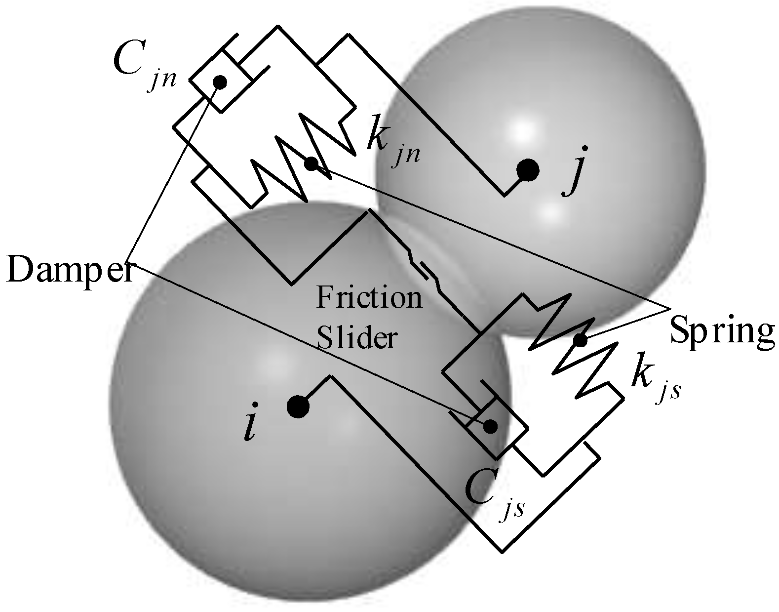
Hereafter, we focus on the contact of particle i with particle j, as shown in Figure 2. Denoting the spring constants in the n, s and b directions as k_jn, k_js, and k_jb(=k_js), respectively, the spring forces e_jn, e_js, and e_jb, are given as in Equation (4). Denoting the damping coefficients in the n, s, and b directions as C_jn, C_js, and C_jb(=C_js), respectively, the damping forces, d_jn, d_js, and d_jb, are given by Equation (5) [17]. Then, increments of the relative displacements after elapsed time Δt in the n, s, and b directions are Δu_jn, Δu_js, and Δu_jb, respectively, and the amounts of contact are u_jn, u_js, and u_jb.

Figure 1. Image of contact condition of two particles in a container.

Figure 1. Image of contact condition of two particles in a container.

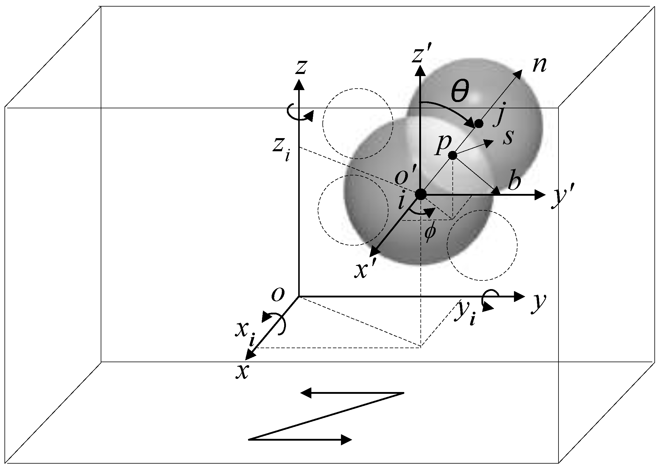
Figure 2. Model for analysis.

Figure 2. Model for analysis.

$${e_{jn}|}_t=k_{jn}\times u_{jn}^{3/2},{e_{js}|}_t=k_{js}\times u_{js}^{3/2},{e_{jb}|}_t=k_{js}\times u_{jb}^{3/2}$$

(4)

$${d_{jn}|}_t=C_{jn}\times u_{jn}^{1/4}\times \mathrm{\Delta }{u}_{jn}/\mathrm{\Delta }t,{d_{js}|}_t=C_{js}\times u_{js}^{1/4}\times \mathrm{\Delta }{u}_{js}/\mathrm{\Delta }t,{d_{jb}|}_t=C_{js}\times u_{jb}^{1/4}\times \mathrm{\Delta }{u}_{jb}/\mathrm{\Delta }t$$

(5)

The spring constant in the n direction, k_jn, is determined from the equation of the Hertzian contact theory for the case of contact between particles [20]. Namely, k_jn is given as in Equation (6). Here, E_i and E_j are the Young’s modules of particles i and j, v_i and v_j are their Poisson’s ratios and r_j and r_j are their radii.

$$k_{jn}=\frac{4}{3}\times \sqrt{\frac{r_i{r}_j}{r_i+r_j}}/\left(\frac{1-{v_i}^2}{E_i}+\frac{1-{v_j}^2}{E_j}\right)$$

(6)

The spring constant in the s direction, k_js is determined as follows, using the ratio of the Young’s modules to the shear modules, ε.

$$k_{js}=\text{ε}\times k_{jn}$$

(7)

$$\text{ε}=1/\{2(1+({\text{ν}}_i+{\text{ν}}_j)/2)\}$$

(8)

Next, the damping coefficient in the n direction, C_jn, is determined by considering the behavior of the particle bounce after contact. Namely, C_jn is adjusted to 1/4 of the critical damping coefficient, as shown in Equation (9). The damping constant in the s direction, C_js is represented by Equation (10).

$$\begin{gathered} C_{jn}=\sqrt{m_{ij}{k}_{jn}}/2 \\ (\because m_{ij}=m_i{m}_j/(m_i+m_j)) \end{gathered}$$

(9)

$$C_{js}=\sqrt{\text{ε}}\times C_{jn}$$

(10)

The spring constant, k_w, between the particle and the wall of the container, is determined from the equation of the Hertzian contact theory for the case of contact between a spherical surface and a plane. Namely, k_w is given as in Equation (11) by substituting ∞ for r_j in Equation (6). Here, E_w is the Young’s module of the container, and v_w is its Poisson’s ratio.

$$k_w=\frac{4}{3}\times \sqrt{r_i}/\left(\frac{1-{{\text{ν}}_i}^2}{E_i}+\frac{1-{{\text{ν}}_w}^2}{E_w}\right)$$

(11)

Material properties are shown in Table 1 for computational conditions.

Table 1. Material property.

Material	Particle	Container
	Carbon Steel	Acrylic
Density (kg/m3)	7873	-
Young’s modulus (MPa)	2.07 × 105	4.90 × 103
Poisson’s ratio	0.26	0.32

Table 1. Material property.

Material	Particle	Container
	Carbon Steel	Acrylic
Density (kg/m3)	7873	-
Young’s modulus (MPa)	2.07 × 105	4.90 × 103
Poisson’s ratio	0.26	0.32

Here we provide a simple explanation of the calculation procedure. We set the time step Δt to be 10⁻⁶ s. The initial arrangement of the particle is random so that contact between particles does not occur inside the container. Then the increments of the displacements and rotational angles of each particle were set to 0. Next, the above gains could be obtained by calculating the free-fall motion of each particle at each time step. Then, acceleration and angular acceleration were obtained using Equations (1)–(5). Each gain at the next time step was calculated from the difference between the displacement obtained from integration of the above acceleration and angular acceleration and that of the previous step. We repeated this procedure at each time step. The particle positions after calculation for t = 1.0 s were set to be at the initial arrangement. Movement of the container began after this initial arrangement. The motion of the container is given as Equation (12), in accordance with the experiment described later.

$$y_w=D\sin (2\text{π}ft)$$

(12)

Particle behavior for 15 s after initial arrangement was calculated.

3. Experimental Apparatus

As shown in Figure 3, the container was placed on a plate with reciprocating block slider crank mechanism. The container used was an acrylic box with width 40 mm, height 40 mm and length 50 mm. To obtain the collision data, metallic plates covered with a piezo film were placed in the container. The distances between the metallic plates, S_d, were 40 mm. The container was made to reciprocate horizontally at the frequencies, f, of 3 Hz, 5 Hz, and 7 Hz. The double amplitudes of the container used, D, were 10 mm, 30 mm, and 50 mm. The voltage values from the piezo film were measured with an oscilloscope.

Figure 3. Experimental apparatus.

Figure 3. Experimental apparatus.

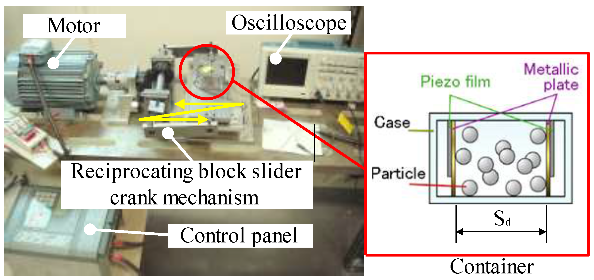
Particles in the container were carbon steel balls. The diameters of those particles, P_d, were 9.5 mm, 12.7 mm, and 19.1 mm. The filling ratios of particles in the container, F_r, were 0%–40% at 5% intervals. The value of the filling ratio was calculated by dividing total particle volume, which was obtained from the number of particles multiplied by the volume of one particle, by the volume of the container.

4. Results of Experiments and Results of Calculations

4.1. Particle Behavior

Figure 4 shows the case in which six carbon steel particles with diameter 19.1 mm were used. The container length was 40 mm, the double amplitude of the container was 50 mm, the frequency was 3 Hz, and the filling ratio was 35%. Figure 4a shows experimental results, and Figure 4b shows results calculated by DEM. In these figures, the behaviors of particles are shown from a certain time at 0.06 s intervals. From Figure 4, it is demonstrated that the behaviors of particles obtained from DEM calculations look like those of experimental results.

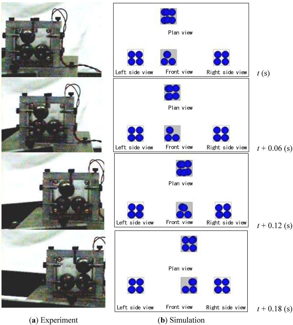
Figure 4. Flow condition (P_d = 19.1 mm, D = 50 mm, f = 3 Hz, F_r = 35%).

Figure 4. Flow condition (P_d = 19.1 mm, D = 50 mm, f = 3 Hz, F_r = 35%).

4.2. Effect of Input Amplitude of Container

Figure 5 shows the relationship between a double amplitude of the container and filling ratio. The diameter of particle was 12.7 mm and the frequency of the container was 7 Hz. Figure 5a shows experimental results, and Figure 5b shows results calculated by DEM. The values in both figures are obtained from the maximum values at 5–15 s after the start of operation. In Figure 5a, the vertical axis represents the maximum voltage obtained from the piezoelectric element, and the horizontal axis represents the filling ratio. Figure 5a shows that the maximum voltage tended to rise so that the reciprocating displacement of the container was large. In Figure 5b(i), the vertical axis represents the maximum velocity of the particle and the horizontal axis represents the filling ratio. Figure 5b(i) shows that the maximum velocity tended to be high when the double amplitude of the container was 50 mm. In Figure 5b(ii), the vertical axis represents the maximum value of work done to the side wall by the particles and the horizontal axis represents the filling ratio. The value of work done to the side wall by the particles is obtained from the contact force and the distance in the normal direction, when the particle comes into contact with the wall. Figure 5b(ii) shows that the maximum value of work done to the side wall was large when the double amplitude of the container was 50 mm. The particle increased momentum because the velocity of the container increased by means of the moved distance of the container. Therefore, it is likely that each value is high when the double amplitude of the container is large because the frequency of the container influences the kinetic energy of the particle. From Figure 5a,b, if the double amplitude with 50 mm at the input amplitude of container is applied in this study, the collision of particles might effectively act on the container.

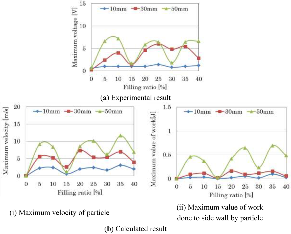
Figure 5. Relationship between double amplitude of container and filling ratio (P_d = 12.7 mm, f = 7 Hz).

Figure 5. Relationship between double amplitude of container and filling ratio (P_d = 12.7 mm, f = 7 Hz).

4.3. Effect of Frequency of Container

Figure 6 shows the relationship between the frequency of container translation and filling ratio. The diameter of the particle was 12.7 mm and the double amplitude of the container was 50 mm. Figure 6a shows experimental results, and Figure 6b shows results calculated by DEM. Figure 6a shows that the maximum voltage tended to rise so that the frequency of the container was high. Figure 6b also show that the maximum velocity and the maximum value of work done to the wall were high when the frequency of the container was high. The frequency of the container also leads to increased container velocity. Therefore, it is likely that each value was high when the frequency of the container was high. From Figure 6, it is apparent that the frequency of the container should be set to a high value. Under such conditions, the effect of the particle might be obtained. However, in the case of filling ratios 15% and 30%, the values of each vertical axis are small.

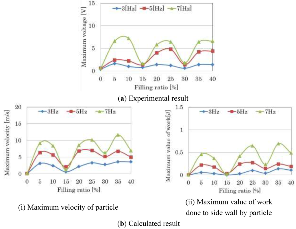
Figure 6. Relationship between frequency of container and filling ratio (P_d = 12.7 mm, D = 50 mm).

Figure 6. Relationship between frequency of container and filling ratio (P_d = 12.7 mm, D = 50 mm).

Next, we focus on particle behaviors with filling ratios 10% and 15%, as shown in Figure 6. Figure 7 shows flow conditions and particle behaviors at 7 Hz with filling ratios of 10% and 15%, respectively. Figure 7 shows that the particles in Figure 7a are the jumping motion and the arrangement of the particles in Figure 7b becomes balanced. Then, the time history response of velocity was examined.

Figure 8 shows the time history response of the velocity in Figure 7, respectively. There are two periodic components in Figure 8a. One is 7 Hz (reference “A” in Figure 8a), and the other is 21 Hz (reference “B” in Figure 8a). Because 7 Hz is the frequency of the container, the particles have collided periodically with the wall. In the case of the other frequency, the collision frequency has increased further. On the other hand, Figure 8b also shows the periodic motion at 7 Hz. It is found that the velocity of Figure 8a is higher than that of Figure 8b. Namely, when the collision frequency of particles and the side wall is higher than the reciprocating frequency of the container, and the flow conditions on this high frequency occur, a high rate of collision is attained. Therefore, it should be possible to obtain the effects of a particle damper by evaluating the flow condition of particles in the container.

Figure 7. Flow conditions (P_d = 12.7 mm, D = 50 mm, f = 7 Hz).

Figure 7. Flow conditions (P_d = 12.7 mm, D = 50 mm, f = 7 Hz).

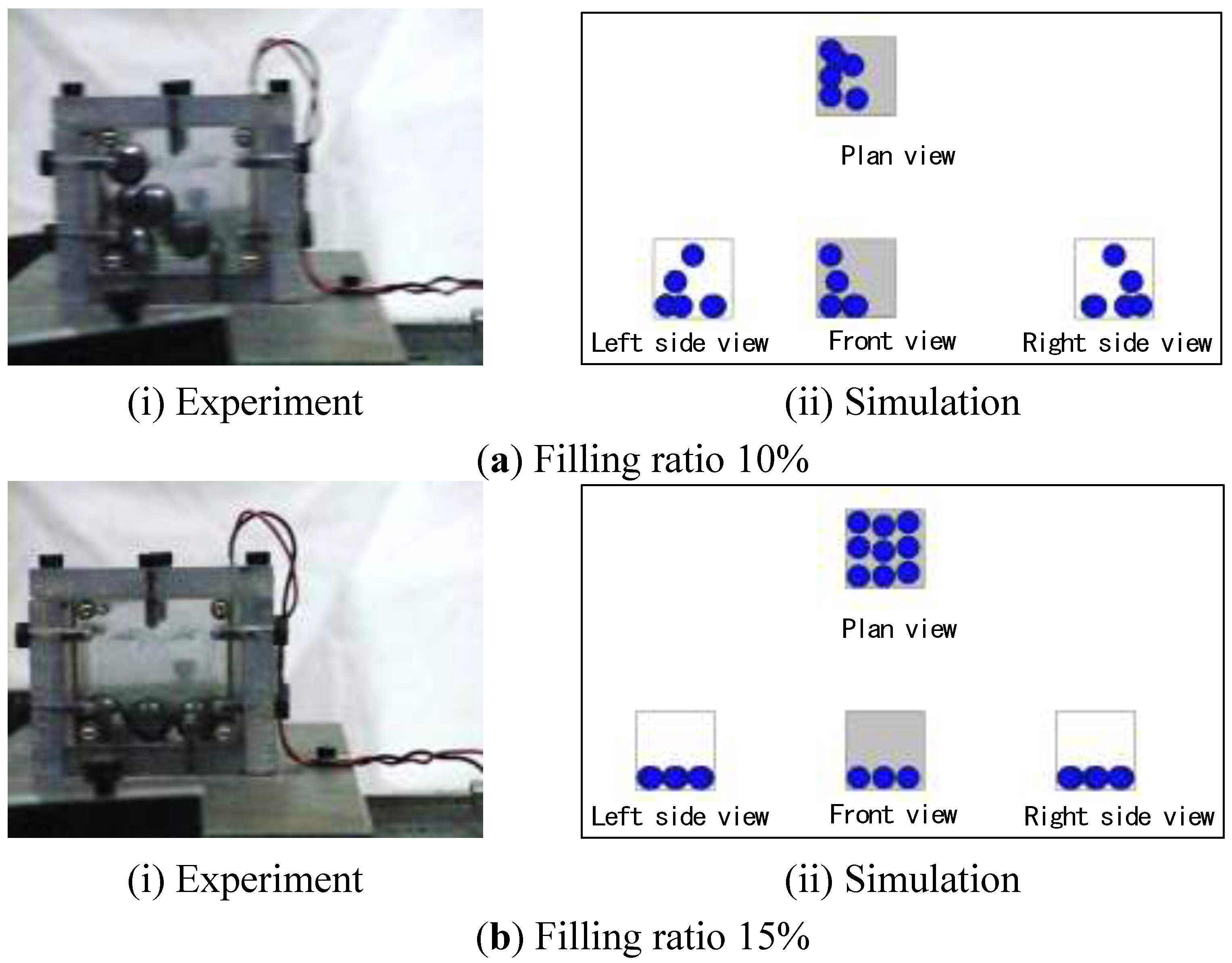
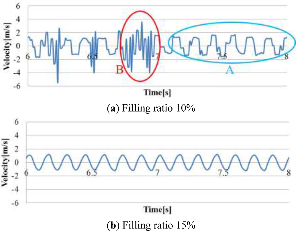
Figure 8. Example of time history response of velocity in Figure 7.

Figure 8. Example of time history response of velocity in Figure 7.

4.4. Effect of Particle Size

Figure 9 shows the relationship between particle size and filling ratio. The double amplitude of the container was 50 mm and the frequency of the container was 7 Hz. Figure 9a shows experimental results, and Figure 9b shows results calculated by DEM. Figure 9a shows the maximum voltage rise depending on the conditions of filling ratio and particle size. Figure 9b shows that the maximum velocity of a 9.5 mm particle was almost constant and its maximum value of work done was smaller than that of the other particle sizes. This can be explained by the fact that 9.5 mm particles can move in the container more freely than particles with larger size. Therefore, the velocity associated with particles of this size is almost constant. Because their mass is also smaller than that of other particles, the kinetic energy of an individual particle is smaller. Therefore, the maximum value of work done is small and constant. Conversely, Figure 9b(ii) shows that the maximum value of work done to a side wall by a particle with diameter 19.1 mm is larger than that of the other particle sizes because its mass is large. However, the tendency of a particle with diameter 19.1 mm is different from experimental results. Particularly, in the case of filling ratio 25%, though the particles are in a balanced arrangement, as in Figure 7b, the maximum value of work done is high in the calculation. Experiment and calculation results both agreed that a particle that was pushed by other particles moved slightly at high-speed several times. It is thought that the piezoelectric element was not able to perceive this slight motion.

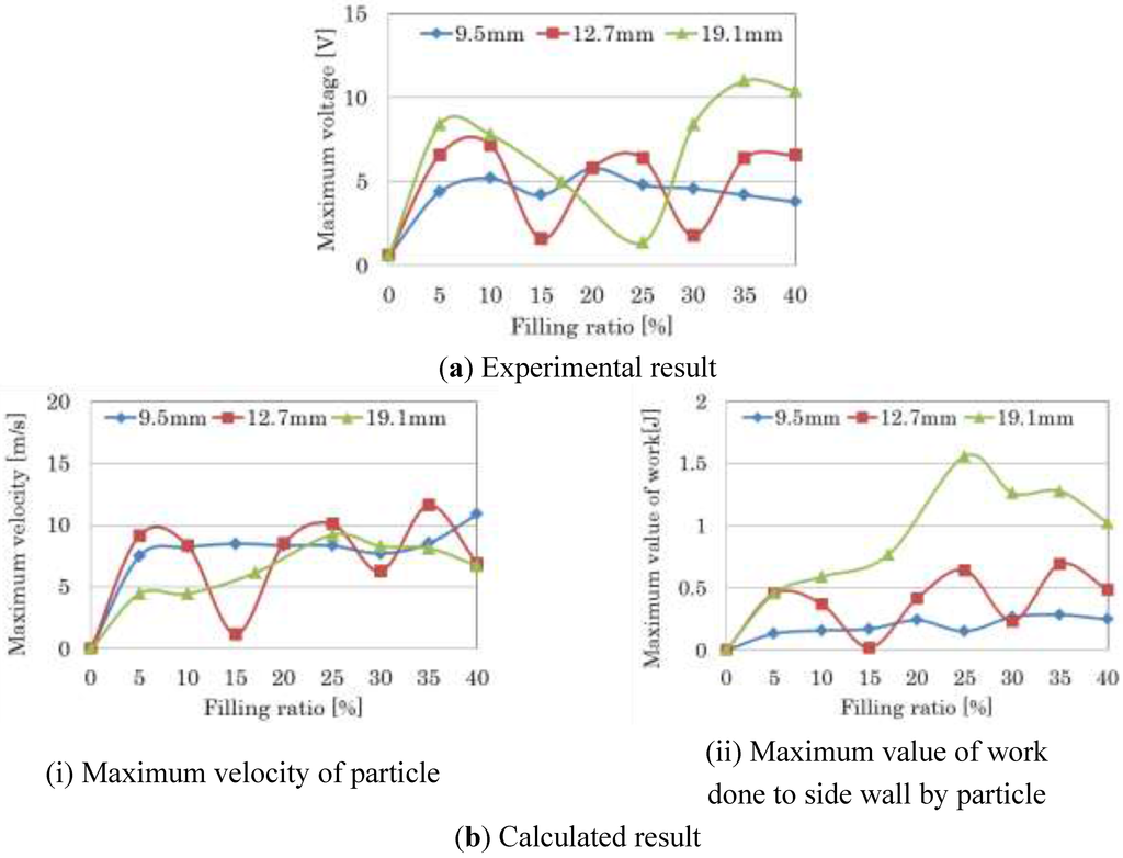
Figure 9. Relationship between particle size and filling ratio (f = 7 Hz, D = 50 mm).

Figure 9. Relationship between particle size and filling ratio (f = 7 Hz, D = 50 mm).

Next, the maximum value of power imparted to side walls by particles was examined. This value is obtained from the amount of work done in 1 s. Figure 10 shows the relationship between a maximum value of power and filling ratio. In Figure 10, the vertical axis represents the maximum value of power to the side walls by a particle. In Figure 10, the maximum value of power from a particle with diameter 19.1 mm is larger than that of the other particle sizes. Particularly, the powers associated with filling ratios of 10% and 35% are high. In these cases, as in Figure 8, the occurrence of flow conditions at high frequency was confirmed. It is thought that the effect of the collision of particles is high. On the other hand, the maximum value of power of filling ratio 25% is low in Figure 10, though the maximum value of work done is high in Figure 9b(ii). Therefore, in this case, there is not a pronounced effect of particle collisions. From Figure 9 and Figure 10, we can infer that an appropriate selection of filling ratio and particle size may lead to particles for damping.

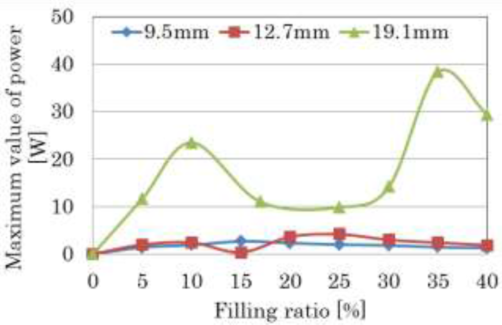
Figure 10. Maximum value of power imparted to side wall by particle in Figure 9b.

Figure 10. Maximum value of power imparted to side wall by particle in Figure 9b.

5. Conclusions

The behavior of particles in the container of the particle damper was examined through experiments using piezoelectric elements and simulations using DEM. The results obtained are as follows:

(1)

Effective collision occurs depending on the combination of particle size and filling ratio. The frequency of particles colliding with the side wall of the container is higher than the reciprocating frequency of the container.

(2)

When the flow condition of the particles is the jumping motion, the particle brings about the effect to the side wall. Inversely, when balanced, the effect is small.

(3)

A simple system using a piezoelectric element is an effective method to obtain the effects of particle collisions.

(4)

The behavior of particles and flow conditions using DEM simulations agreed well with experimental results. It is possible to evaluate the effect of particle collisions using DEM.

References

- Nagashima, T.; Sato, T.; Tanaka, K. Vibration Control Using an Impact Damper System—Comparison between Translating Impactor and Rotating Impactor, and Improvement of Rotating Impactor. J. Environ. Eng. 2010, 5, 402–416. [Google Scholar] [CrossRef]
- Duncan, M.R.; Wassgren, C.R. The damping performance of a single particle impact damper. J. Sound Vib. 2005, 286, 123–144. [Google Scholar] [CrossRef]
- Friend, R.D.; Kinra, V.K.; Krousgrill, C.M. Particle impact damping. J. Sound Vib. 2000, 233, 93–118. [Google Scholar] [CrossRef]
- Inoue, M.; Yokomichi, I.; Hiraki, K. Particle damping with granular materials for multi degree of freedom system. Shock Vib. 2011, 18, 245–256. [Google Scholar] [CrossRef]
- Araki, Y.; Yokomichi, I.; Inoue, J. Impact Damper with Granular Materials 2nd Report, Both Sides Impact in a Vertical Oscillating System. Bull. JSME 1985, 28, 1466–1472. [Google Scholar] [CrossRef]
- Lu, Z.; Lu, X.; Masri, S.F. Studies of the performance of particle dampers under dynamic loads. J. Sound Vib. 2010, 329, 5415–5433. [Google Scholar] [CrossRef]
- Saeki, M. Impact Damping with Granular Materials in a Horizontally Vibrating system. J. Sound Vib. 2002, 251, 153–161. [Google Scholar] [CrossRef]
- Saeki, M. Analytical study of multi-particle damping. J. Sound Vib. 2005, 281, 1133–1144. [Google Scholar] [CrossRef]
- Sánchez, M.; Carlevaro, C.M. Nonlinear dynamic analysis of an optimal particle damper. J. Sound Vib. 2013, 332, 2070–2080. [Google Scholar] [CrossRef]
- Cundall, P.A.; Strack, O.D.L. A Discrete Numeric Model for Granular Assemblies. Geotechnique 1979, 29, 47–65. [Google Scholar] [CrossRef]
- Cleary, P.W.; Sawley, M.L. DEM modelling of industrial granular flows: 3D case studies and the effect of particle shape on hopper discharge. Appl. Math. Model. 2002, 26, 89–111. [Google Scholar] [CrossRef]
- Balevičius, R.; Kačianauskas, R.; Mróz, Z.; Sielamowicz, I. Analysis and DEM simulation of granular material flow patterns in hopper models of different shapes. Adv. Powder Technol. 2011, 22, 226–235. [Google Scholar] [CrossRef]
- Mishra, B.K.; Rajamani, R.K. Motion Analysis in Tumbling Mills by the Discrete Element Method. Kona 1990, 8, 92–98. [Google Scholar] [CrossRef]
- Yamane, K.; Sato, T.; Tanaka, T.; Tsuji, Y. Computer Simulation of Tablet Motion in Coating Drum. Pharm. Res. 1995, 12, 1264–1268. [Google Scholar] [CrossRef] [PubMed]
- Paul, W. Cleary, Predicting Charge Motion, Power Draw, Segregation and Wear in Ball Mills Using Discrete Element Methods. Miner. Eng. 1998, 11, 1061–1080. [Google Scholar]
- Kano, J.; Chujo, N.; Saito, F. A Method for Simulating the Three-Dimensional Motion of Balls under the Presence of a Powder Sample in a Tumbling Ball Mill. Adv. Powder Technol. 1997, 8, 39–51. [Google Scholar] [CrossRef]
- Tsuji, Y.; Ishida, T.; Tanaka, T. Lagrangian Numerical Simulation of Plug Flow of Cohesionless Particles in a Horizontal Pipe. Powder Technol. 1992, 71, 239–250. [Google Scholar] [CrossRef]
- Kawamoto, Y.; Kataoka, M.; Uekusa, M.; Terumichi, Y. Behavior of Two Kinds of Particles in Rotary Barrel with Planetary Rotation. Multibody Syst. Dyn. 2004, 12, 187–207. [Google Scholar] [CrossRef]
- Takahashi, Y.; Kataoka, M.; Uekusa, M.; Terumichi, Y. Behavior of Three Kinds of Particles in Rotary Barrel with Planetary Rotation. Multibody Syst. Dyn. 2005, 13, 195–209. [Google Scholar] [CrossRef]
- Timoshenko, S.; Goodier, J.N. Theory of Elasticity, 2nd ed.; Mcgraw-Hill Kōgakusya: Tokyo, Japan, 1951; pp. 372–384. [Google Scholar]
© 2015 by the authors; licensee MDPI, Basel, Switzerland. This article is an open access article distributed under the terms and conditions of the Creative Commons Attribution license (http://creativecommons.org/licenses/by/4.0/).