Article

An Analytical Method for Generating Determined Torque Ripple in Synchronous Machines with Surface Magnets by Harmonic Current Injection

Karlsruhe Institut of Technology, 76131 Karlsruhe, Germany
*
Author to whom correspondence should be addressed.
Machines 2020, 8(2), 32; https://doi.org/10.3390/machines8020032
Submission received: 30 April 2020 / Revised: 29 May 2020 / Accepted: 29 May 2020 / Published: 8 June 2020

Abstract

:
In this paper, we present a new analytical method to calculate the required amplitudes and phase angles of the injected harmonic currents, to generate a determined torque ripple for synchronous machines with surface-mounted permanent magnets. First, we described the machine equations as a function of the phase current and the back electromotive force. We then introduced a new asymmetrical power system. After combining the equations, we established a linear system of equations. The solution of the equation system yielded the amplitudes and phase angles of the harmonic currents to be injected. Finally, we validated the method with several finite element method simulations. With this method, a previously defined torque ripple could be generated very accurately for synchronous machines with surface magnets.

1. Introduction

Permanent-magnet synchronous machines (PMSM) have largely established themselves in recent years as electric traction machines (ETM), thanks to their high power density and low maintenance requirements. They meet the requirements for hybrid electric vehicles (HEV) and purely electric vehicles (EV) better than any other system [1]. Advances in converter technology have made their use much easier [2].
PMSM, like almost every other system for ETM, do not have a smooth torque curve even in the stationary state. This torque ripple is one of the main reasons for speed fluctuations and generates vibrations that can excite the resonance frequencies of other components. This can lead to strong noise and vibration emissions [3].
In recent years, many publications have dealt with the reduction of the torque ripple of PMSM. Many good results have been achieved in this area through constructive modifications, like the distribution of the winding [4], single-layer winding or double-layer winding [5], magnetic pole, and anchor-slot design [6]. However, these methods are mostly limited to the reduction of the cogging torque.
Another approach to reduce torque ripple is control intervention. One variant of this is harmonic current injection (HCI). By injecting current harmonics onto the sinusoidal supply current, it reduces the fluctuations in torque at the output side of the ETM [7,8,9].
Current methods try to reduce torque ripple as close as possible to zero. In general, the electric drive train of a HEV or EV consists of more than just the ETM. Of course, it should be aimed at an ETM without torque ripple, in order to reduce noise and vibration emissions. Nevertheless, it can also be advantageous to generate a certain torque ripple on the output side of the ETM. For example, to reduce vibrations coming from other sources (such as gearboxes, differentials, or auxiliary units) by means of counter-phase excitation. Alternatively, to imitate the low-frequency noise spectrum of an internal combustion engine, which is far more accepted by the population than the narrow-banded, high-frequency noise spectrum of electric drives.
This is the starting point of this publication, which presents an analytical method for determining the amplitudes and phase angles of current harmonics for synchronous machines with surface magnets (SPMSM) in order to obtain a desired torque fluctuation.

2. Fundamentals

2.1. Machine Equations for Synchronous Machines with Surface-Mounted Permanent Magnets

The mathematical models for the stator voltages of a PMSM are described in detail in the literature [9,10,11,12]. The total torque of the machine can be divided into three parts, which are more or less significant, depending on the machine type [13]:
T e m t = T a l i g n t + T r e l t + T c o g t .
T a l i g n t stands for the electromagnetic torque from the Lorentz force, T r e l t represents the reluctance torque, and T c o g t is the cogging torque.
In the following, we do not examine the cogging torque in detail. Although it contributes to the torque oscillations, it is only dependent on the stator shape and rotor flux. Those are generally constant for PMSM and, therefore, cannot be influenced by external control interventions. The reluctance torque contributes both, to the constant torque and to the torque ripple, and can be calculated by the following equation [13]:
T r e l t = p 2 1 2 i a 2 d L a d ϑ + 1 2 i b 2 d L b d ϑ + 1 2 i c 2 d L c d ϑ + i a i b d M a b d ϑ + i b i c d M b c d ϑ + i a i c d M a c d ϑ
where p stands for the number of poles, i a b c represents the phase currents, L a b c represents the self-inductance of the phases, M a b c , b c a represents the mutual inductance between the phases, and ϑ is the rotating angle of the rotor.
For SPMSM, it applies approximately that the inductivities of the rotor are independent of the angle of rotation. For that reason, we can neglect the reluctance part of the torque. The remaining part of the torque can be calculated, according to [9,14], by:
T a l i g n t = 1 ω r · i a u p , a + i b u p , b + i c u p , c .
Here, u p , a b c is the counter electromotive force, also known as back electromotive force (or back EMF), generated by the rotation of the permanent magnets of the rotor in the magnetic field of the stator [15], i a b c represents the phase currents, and ω r is the rotational speed of the stator field or rotor.

2.2. Power Supply System

For the operation of a three-phase machine, a supply current system is required that is divided into phases i a ,   i b and i c . In the considered case of a star connection without a neutral conductor, the three phases have to match the condition:
i a + i b + i c = 0 .
In practice, the symmetrical current system has been established as the preferred solution. This is described in detail in literature [10,15,16]. A uniform sine wave with a phase shift of 120 degrees is fed into the three phases. This system is subject to the restriction that no harmonic currents with a frequency corresponding to a multiple of three may be injected into the system, otherwise the condition of Equation (4) is violated.
If we abandon the requirement of a symmetrical current profile, it is possible to use an asymmetrical current system. In this case, we still feed the fundamental oscillations symmetrically into the system with a phase shift of 120 degrees. However, since injected harmonics do not require an identical shape in all three phases, it is possible to feed harmonic currents with a frequency multiple of three into the system without violating the condition of Equation (4).
If the set N a s y m contains all harmonic components we want to inject into the current system, we can describe the asymmetric current system by Equation (5).
i a , b , c = n     N a s y m i ^ n · sin n ω e t 2 3 π s + δ n
where s = 0 ,   1 ,   2 define the phases a, b, or c, i ^ n and δ n define the respective amplitude and phase shift of the injected harmonic current, and ω e describes the angular frequency of the fundamental oscillation. Figure 1 shows the examples of a symmetrical and an asymmetrical current system with the values from Table 1.
The advantage of a symmetrical current system is that only a limited spectrum of harmonics can be generated in torque. For the compensation of torque fluctuations by a classical harmonic current injection, this spectrum is sufficient.
The advantage of the asymmetrical current system lies in the fact that any harmonic oscillation can be generated in the torque and, thus, any required torque fluctuation can be generated. It, therefore, makes sense to combine both systems and thereby use both strengths. The following equation provides the combined current system in the appropriate form:
i a = j N s y m Î s y m , j sin j ω e t + γ s y m , j + k N a s y m Î a s y m , k sin k ω e t + γ a s y m , k i b = j N s y m Î s y m , j sin j ω e t 2 3 π + γ s y m , j + k N a s y m Î a s y m , k sin k ω e t 2 3 π + γ a s y m , k i c = j N s y m Î s y m , j sin j ω e t 4 3 π + γ s y m , j + k N a s y m Î a s y m , k sin k ω e t 4 3 π + γ a s y m , k .

2.3. Back EMF

The rotation of the permanent magnets induces voltages in the stator coils. These voltages can be measured between the star point and the corresponding phase in a PMSM operating with no load. Neglecting the saturation effects in the iron, this voltage corresponds exactly to the counter electromotive force [13].
Since the voltage is not perfectly sinusoidal, we approximate its shape by a Fourier series in order to bring the analytical equations into a suitable form. This leads to the following representation for the back EMF:
u p , a = μ N μ Û p , μ sin μ ω e t u p , b = μ N μ Û p , μ sin μ ω e t 2 3 π u p , c = μ N μ Û p , μ sin μ ω e t 4 3 π .
At this point, we note that many real machines are designed for an almost sinusoidal back EMF. Therefore, for analytical calculations, the first elements of the series are often sufficient to make well-founded statements.

2.4. Formulation of the Electromagnetic Torque Resulting from the Lorentz Force

If we now insert Equations (6) and (7) into Equation (3), a formulation is obtained for the electromagnetic torque resulting from the Lorentz force:
T a l i g n t = 1 ω r · ( s = 0 2 ( j N s y m Î s y m , j sin j ( ω e t 2 3 π s ) + γ s y m , j + k N a s y m Î a s y m , k sin k ω e t 2 3 π s + γ a s y m , k ) · μ N μ Û p , μ sin μ ω e t 2 3 π s )
Reorganization of the sums brings:
T a l i g n t = 1 ω r · ( s = 0 2 ( μ N μ j N s y m Î s y m , j Û p , μ sin j ( ω e t 2 3 π s ) + γ s y m , j sin μ ω e t 2 3 π s + μ N μ k N a s y m Î a s y m , k Û p , μ sin k ( ω e t 2 3 π s ) + γ a s y m , k sin ( μ ( ω e t 2 3 π s ) ) ) )
The combination of the trigonometric terms and resolution of the outermost sum yields:
T a l i g n t = 1 ω r · ( μ N μ j N s y m Î s y m , j Û p , μ ( cos j μ ω e t + γ s y m , j cos j + μ ω e t + γ s y m , j + cos j μ ω e t + γ s y m , j j μ 2 3 π cos j + μ ω e t + γ s y m , j j + μ 2 3 π + cos j μ ω e t + γ s y m , j j μ 2 3 π cos j + μ ω e t + γ s y m , j j + μ 2 3 π ) + μ N μ k N a s y m Î a s y m , k Û p , μ ( cos k μ ω e t + γ a s y m , k cos k + μ ω e t + γ a s y m , k + cos k μ ω e t + γ a s y m , k k μ 2 3 π cos k + μ ω e t + γ a s y m , k k + μ 2 3 π + cos k μ ω e t + γ a s y m , k k μ 4 3 π cos k + μ ω e t + γ a s y m , k k + μ 4 3 π ) )
Transformation of Equation (10), using the angle sum and difference identities, yields the following form:
T a l i g n t = 3 2 ω r ( μ N μ j N s y m ( Î s y m , j Û p , μ sin γ s y m , j sin j ±   μ ω e t + Î s y m , j Û p , μ cos γ s y m , j cos j ±   μ ω e t ) + μ N μ k N a s y m ( Î a s y m , k Û p , μ sin γ a s y m , k sin k ±   μ ω e t + Î a s y m , k Û p , μ cos γ a s y m , k cos k ±   μ ω e t ) )

3. Approach

3.1. Formulation of the System of Linear Equations

First, we must bring the nominal torque curve with its fluctuations into the appropriate shape. Here, the decomposition into a Fourier series is suitable:
T e m t = T n o m t = l N n o m T ^ n o m , l · sin l ω e t + γ n o m , l .
A subsequent transformation using the angle sum and difference identities for trigonometric functions yields the form:
T n o m t = l N n o m T ^ n o m , l · cos γ n o m , l · sin l ω e t + T ^ n o m , l · sin γ n o m , l · cos l ω e t .
We assumed to know the cogging torque and neglect the reluctance torque for SPMSM, so we convert Equation (1) as follows:
T a l i g n t = T n o m t T c o g t .
Similar to the nominal torque, we used a Fourier series decomposition, the angle sum, and difference identities to create the following structure for T c o g t :
T c o g t = g N c o g T ^ c o g , g · cos γ c o g , g · sin g ω e t + T ^ c o g , g · sin γ c o g , g · cos g ω e t .
Now, we represent Equation (14) by Equations (11), (13), and (15) as a linear combination of the independent vectors sin n ω e t and cos n ω e t |   n N n o m N c o g . A coefficient comparison between the left and the right side yields a system of equations with 2 n equations of the form:
U · x _ = h _
with
x _ = Î s y m , 1 sin γ s y m , 1 Î s y m , 1 cos γ s y m , 1 Î s y m , j m a x sin γ s y m , j m a x Î s y m , j m a x cos γ s y m , j m a x Î a s y m , 1 sin γ a s y m , 1 Î a s y m , 1 cos γ a s y m , 1 Î a s y m , k m a x sin γ a s y m , k m a x Î a s y m , k m a x cos γ a s y m , k m a x
and
h _ = T ^ n o m , 1 cos γ n o m , 1 T ^ c o g , 1 cos γ c o g , 1 T ^ n o m , 1 sin γ n o m , 1 T ^ c o g , 1 sin γ c o g , 1 T ^ n o m , l m a x cos γ n o m , l m a x T ^ c o g , g m a x cos γ c o g , g m a x T ^ n o m , l m a x sin γ n o m , l m a x T ^ c o g , g m a x sin γ c o g , g m a x .
A general representation of the matrix U , without defined sets N s y m , N a s y m , and N μ , is not trivial and should not be done here.

3.2. Solvability of the Linear System of Equations
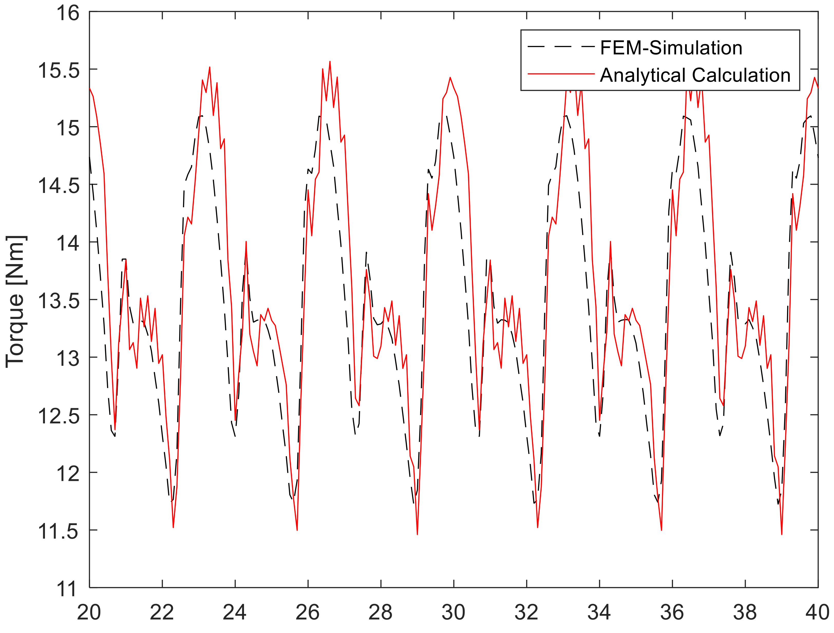
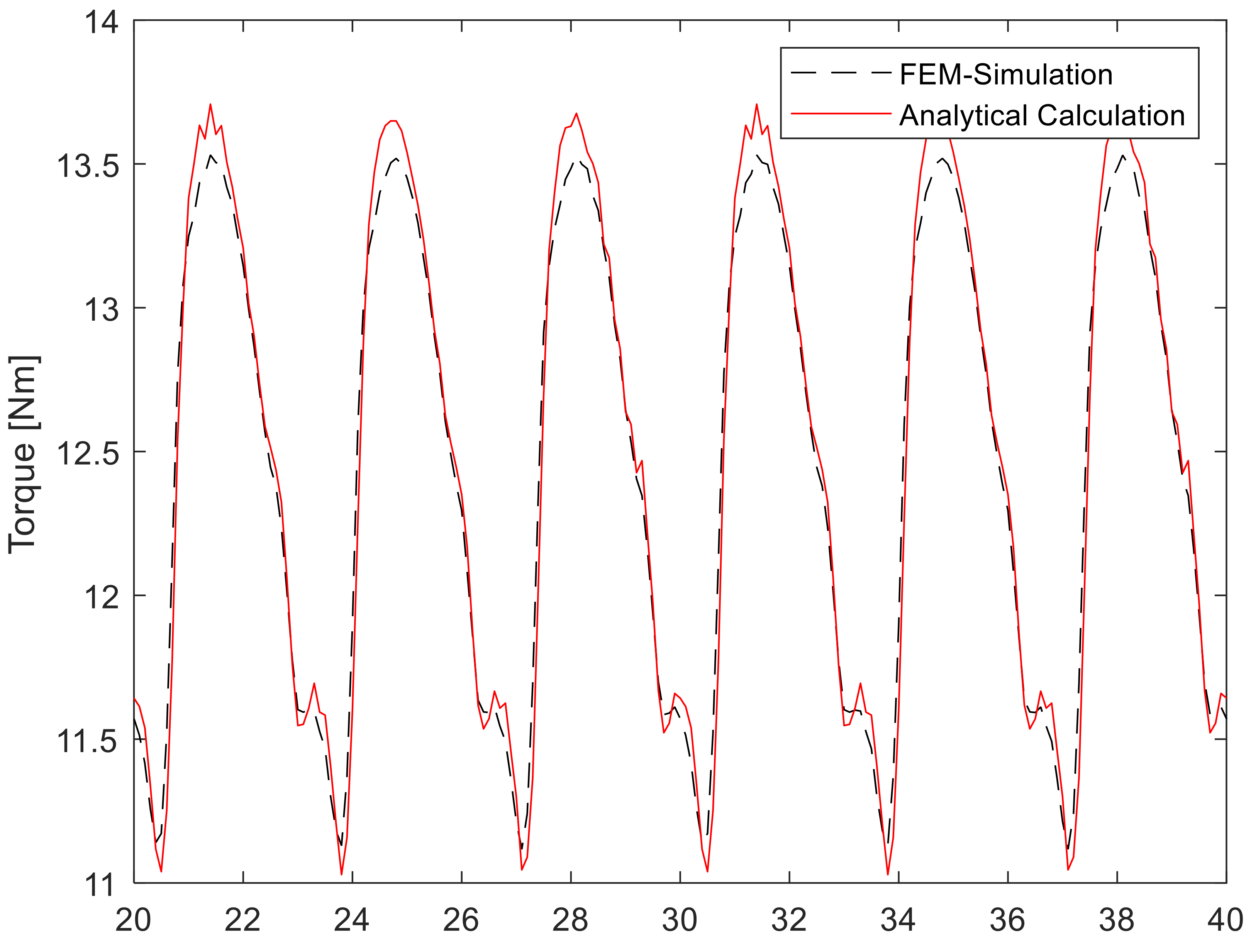
To yield a solution for the equation system Equation (16) U must be regular, thus quadratic and invertible. U is quadratic if the number of coefficient comparisons corresponds to the number of entries of the vector x _ . This is the case if the sum of the double cardinality of the sets N s y m and N a s y m corresponds to the cardinality of the union of N n o m and N c o g :
2 · N s y m + 2 · N a s y m = N n o m N c o g .
U can be inverted if its determinant does not disappear, which must be checked for each individual case.

4. Validation

4.1. Machine Parameters and Validation of the Torque Calculation Method

To check the approach of Section 3 in principle, we simulated two machines with Ansys® Electromagnetics Suite 19.0.0 - Maxwell 2D and RMxprt and compared the results of the FEM (finite element method) simulation with the results of the described method.
Table 2 shows some of the setting parameters from the FEM simulation. Table 3 describes the operating point under investigation and Table 4 and Table 5 give the associated values for the cogging torque and back EMF from the FEM analysis.
Figure 2 and Figure 3 show the torque curve for machine A and B, calculated by the FEM model, as well as the calculation method presented in Section 2 for the operating point from Table 3. Figure 4 and Figure 5 show the corresponding fast Fourier transformation (FFT) analysis of the torque curves from Figure 2 and Figure 3. The constant part of the torque is not shown but given as a numerical value for reasons of visibility. For machine A, the deviations between analytical calculation and FEM-simulation harmonic amplitudes was less than 1.6% of the constant torque. For machine B, they were less than 0.5% of the constant torque.

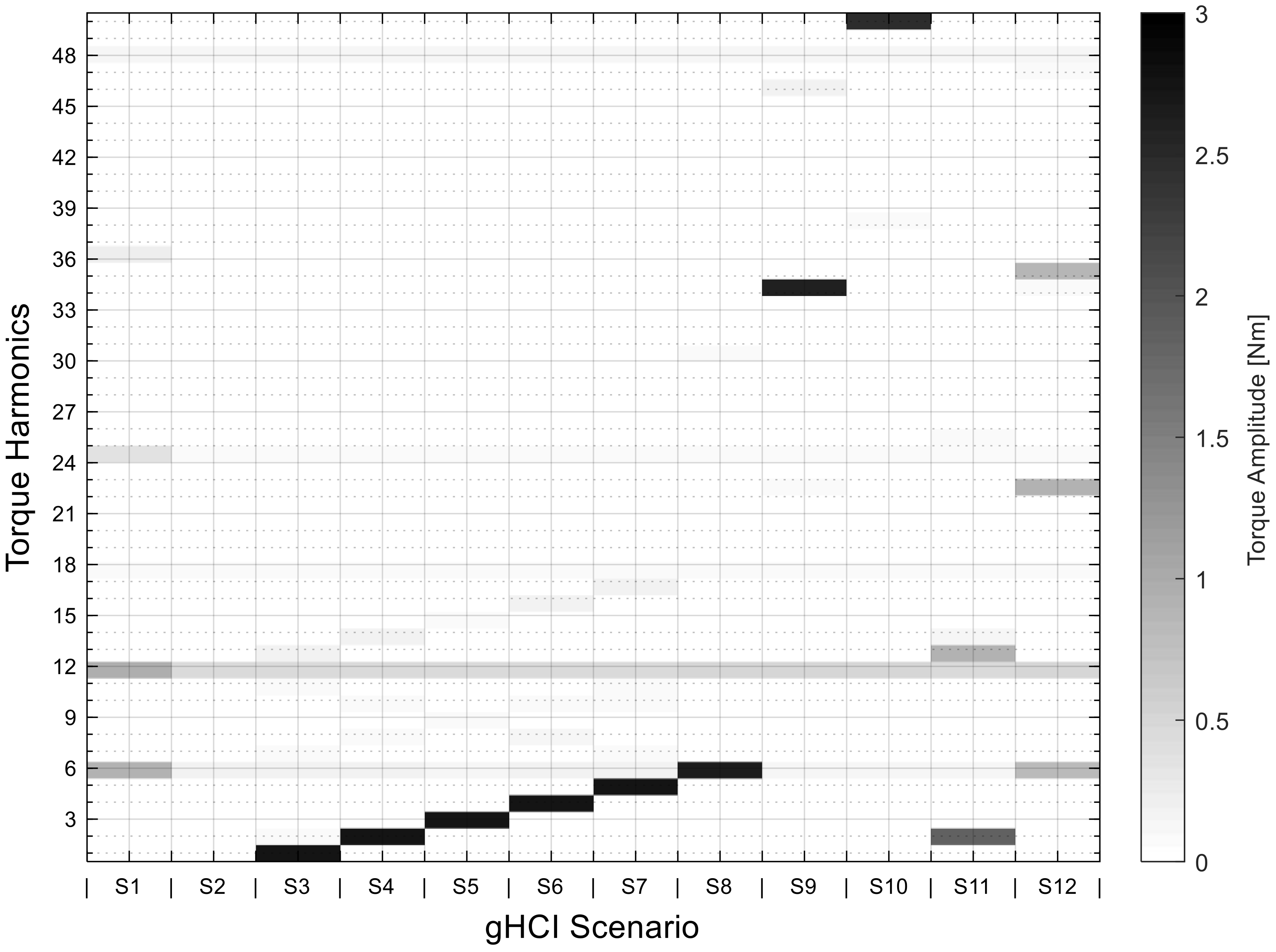
4.2. Validation of Generative Harmonic Current Injection

We tested 12 scenarios for machine A in the following, in which we wanted to receive a very specific ripple in the torque. Table 6 lists the scenarios together with the sets N s y m and N a s y m , which were injected into the current as additional harmonic waves. All amplitudes of harmonics in torque that are not listed in the table should automatically be set to zero for the respective scenario.
The torque curves from the FEM simulations were analyzed by an FFT, as in Section 4.1. This was used to check whether the torque fluctuations required in the respective scenarios could be generated. Figure 6 shows the results of the FFT analysis for each individual scenario. S1 and S2 operate as reference cases and show the results of the FFT when nothing is injected or harmonics are injected to suppress torque fluctuation. The figure also shows that in addition to the required torque fluctuations, further harmonics with non-negligible amplitude were generated.

5. Conclusions

The results of the validation in Section 4.1 showed that the calculation of the torque via Equation (3) corresponded well with the results from the far more complex and computationally more elaborate FEM simulation. For the constant torque, the deviations were less than 2% for both machines. Individual harmonics, such as the sixth harmonic of machine A, may have had deviations of 20% from the corresponding harmonic of the FEM simulation, but in absolute terms this corresponded to a deviation of only 1.5% from the constant torque. As Figure 4 and Figure 5 show, the amplitudes of the harmonics can vary both upwards and downwards. A general trend was not recognizable. However, it can be said that, except for one outlier, the deviations became smaller the higher the order of the corresponding harmonic became. The reluctance torque may well have caused deviations between the analytical calculation and the FEM simulation, since this was calculated in the FEM simulation but neglected in the analytical calculation. The assumption in Section 2.1 that the reluctance torque could be neglected for synchronous machines with surface magnets was confirmed by the small deviations. The results from the validation suggest that the analytical calculation of the electromagnetic torque from the Lorentz force is justified by Equation (11).
The results of Figure 6 show that we can generate the harmonics in torque demanded in advance with a sufficiently large amplitude. In addition to the desired ones, we can compensate the undesired fluctuations that occur in the machine without current injection as far as possible to zero (see scenario 1 and scenario 2). However, the results also show that, in addition to the desired harmonic waves, parasitic harmonics of low amplitude were also generated which had not previously appeared in the torque spectrum. These occurred from the interaction of the injected harmonics in the current with the fundamental wave of the back EMF. Therefore, as few harmonics as possible should be injected into the current, so as few oscillations as possible can interact with each other to generate additional harmonics. In general, it has to be considered whether the benefit generated by the desired harmonic waves justifies these additional fluctuations for every single machine.

6. Summary

In this paper, we presented an analytical method that allowed the generation of a very specific torque ripple by HCI for SPMSM. First, we described the machine equations as a function of the phase current and the back EMF. Then we introduced a new asymmetrical power system, which enabled higher harmonics to be injected into the torque, which was a multiple of three. After combining the equations, we established a linear system of equations. For this purpose, we converted the different components in such a way that a coefficient comparison between the different sine and cosine terms was possible.
The solution of the linear equation system yielded the amplitudes and phase angle of the respective harmonics, which must be injected into the phase current. Next, we discussed the requirements under which the linear system of equations could be solved.
This was followed by the validation of the analytical method by comparison with a FEM simulation. First, we compared the torque of the FEM simulation with the analytical calculation without harmonic currents being injected. Although we observed slight deviations, they were within an acceptable range. The next step was to inject higher harmonic currents in order to obtain the required torque ripple on the output side of the machine. Here we showed that the FEM simulation came very close to the required torque curves and, thus, validated the presented analytical method.

Author Contributions

Conceptualization, M.V.; methodology, M.V.; software, D.H.; validation, D.H.; resources, F.G.; writing—original draft preparation, M.V.; writing—review and editing, D.H. and F.G.; visualization, M.V.; supervision, F.G.; project administration, F.G.; All authors have read and agreed to the published version of the manuscript.

Funding

This research received no external funding.

Acknowledgments

We acknowledge support by the KIT-Publication Fund of the Karlsruhe Institute of Technology.

Conflicts of Interest

The authors declare no conflict of interest.

References

  1. Zeraoulia, M.; Benbouzid, M.E.H.; Diallo, D. Electric Motor Drive Selection Issues for HEV Propulsion Systems: A Comparative Study. IEEE Trans. Veh. Technol. 2006, 55, 1756–1764. [Google Scholar] [CrossRef] [Green Version]
  2. Kimura, T.; Saitou, R.; Kubo, K.; Nakatsu, K.; Ishikawa, H.; Sasaki, K. High-power-density inverter technology for hybrid and electric vehicle applications. Hitachi Rev. 2014, 63, 42–47. [Google Scholar]
  3. Holtz, J.; Springob, L. Identification and compensation of torque ripple in high-precision permanent magnet motor drives. IEEE Trans. Ind. Electron. 1996, 43, 309–320. [Google Scholar] [CrossRef] [Green Version]
  4. Magnussen, F.; Thelin, P.; Sadarangani, C. Performance evaluation of permanent magnet synchronous machines with concentrated and distributed windings including the effect of field-weakening. In Proceedings of the Second International Conference on Power Electronics, Machines and Drives (PEMD 2004), Edinburgh, UK, 31 March–2 April 200; p. v2-679. [CrossRef]
  5. Bianchi, N.; Bolognani, S.; Pre, M.D.; Grezzani, G. Design considerations for fractional-slot winding configurations of synchronous machines. IEEE Trans. Ind. Appl. 2006, 42, 997–1006. [Google Scholar] [CrossRef]
  6. Chung, D.-W.; You, Y.-M. Cogging Torque Reduction in Permanent-Magnet Brushless Generators for Small Wind Turbines. J. Magn. 2015, 20, 176–185. [Google Scholar] [CrossRef] [Green Version]
  7. Favre, E.; Cardoletti, L.; Jufer, M. Permanent-magnet synchronous motors: A comprehen-sive approach to cogging torque suppression. IEEE Trans. Ind. Appl. 1993, 29, 1141–1149. [Google Scholar] [CrossRef]
  8. Najmabadi, A.; Xu, W.; Degner, M. A Sensitivity Analysis on the Fifth and the Seventh Harmonic Current Injection for Sixth Order Torque Ripple Reduction. In Proceedings of the IEEE International Electric Machines and Drives Conference (IEMDC), Miami, FL, USA, 21–24 May 2017; pp. 1–8. [Google Scholar]
  9. Zhu, Z.Q.; Wu, L.J.; Xia, Z.P. An Accurate Subdomain Model for Magnetic Field Computation in Slotted Surface-Mounted Permanent-Magnet Machines. IEEE Trans. Magn. 2010, 46, 1100–1115. [Google Scholar] [CrossRef]
  10. Hanselman, D. Brushless Permanent Magnet Motor Design; Magna Physics Pub: Lebanon, OH, USA, 2006. [Google Scholar]
  11. Pyrhönen, J.; Hrabovcová, V.; Jokinen, T.; Niemelä, H. Design of Rotating Electrical Machines; Reprinted; Wiley: Chichester, UK, 2010. [Google Scholar]
  12. Schröder, D. Elektrische Antriebe–Grundlagen. Mit Durchgerechneten Übungs- und Prüfungsaufgaben; 5., erw. Aufl.; Springer: Berlin/Heidelberg, Germany, 2013. [Google Scholar]
  13. Farshadnia, M. Advanced Theory of Fractional-Slot Concentrated-Wound Permanent Magnet Synchronous Machines; Springer: Singapore, 2018. [Google Scholar]
  14. Chen, Z.; Li, Z.; Ma, H. A harmonic current injection method for electromagnetic torque ripple suppression in permanent-magnet synchronous machines. Int. J. Appl. Electromagn. Mech. 2017, 53, 327–336. [Google Scholar] [CrossRef]
  15. Krause, P.C.; Wasynczuk, O.; Sudhoff, S.D.; Pekarek, S. Analysis of Electric Machinery and Drive Systems, 3rd ed.; Wiley IEEE Press: Hoboken, NJ, USA, 2013. [Google Scholar]
  16. Schröder, D. Elektrische Antriebe–Regelung von Antriebssystemen; 4. Auflage; Springer: Berlin/Heidelberg, Germany, 2015. [Google Scholar]
Figure 1. Symmetrical and asymmetrical current system in comparison.
Machines 08 00032 g001
Figure 2. Torque curve of machine A.
Machines 08 00032 g002
Figure 3. Torque curve of machine B.
Machines 08 00032 g003
Figure 4. Frequency spectrum of the torque curve of machine A.
Machines 08 00032 g004
Figure 5. Frequency spectrum of the torque curve of machine B.
Machines 08 00032 g005
Figure 6. Results of the Fourier transformed torque ripple of the 12 generative harmonic current injection (gHCI) scenarios of machine A.
Machines 08 00032 g006
Table 1. Example values for Figure 1.
n Î n δ n
1100
22 π 4
410
50.50
70.25 π 2
80.125 π
100.06250
Table 2. Excerpt of the machine parameters from the simulation.
Machine AMachine B
Number of Poles44
Number of Stator Slots2412
Outer Diameter of Stator120 mm100 mm
Inner Diameter of Stator75 mm50 mm
Length of Stator Core65 mm100 mm
Minimum Air Gap0.5 mm0.5 mm
Residual Flux Density0.96 Tesla0.96 Tesla
Table 3. Investigated operating point.
excitation frequency ω e 2 π · 50 Hz
phase angle γ 1 0.2
current amplitude Î 1 12 A
Table 4. Amplitudes of the back electromotive force for machine A and B.
Amplitude in V
Machine AMachine B
Û p , 1 21.93111.53
Û p , 5 −5.0213.39
Û p , 7 4.803.39
Û p , 11 −8.10−2.10
Û p , 13 −1.61−2.07
Table 5. Amplitudes and phases of the Fourier transformed cogging torque.
Amplitude in NmPhase in Rad
Machine AMachine B Machine AMachine B
T ^ cog , 6 0.00210.0000 γ c o g , 6 1.220.00
T ^ c o g , 12 0.31020.2246 γ c o g , 12 1.761.76
T ^ c o g , 18 0.00310.0374 γ c o g , 18 −1.57−1.29
T ^ c o g , 24 0.37020.1402 γ c o g , 24 −1.19−1.19
T ^ c o g , 30 0.00110.0691 γ c o g , 30 1.88−1.10
T ^ c o g , 36 0.24700.0000 γ c o g , 36 2.150.00
T ^ c o g , 42 0.00000.0241 γ c o g , 42 0.002.23
Table 6. List of the 12 scenarios examined for machine A.
ScenarioRequired Torque RippleInjected Harmonics
1First reference scenario: simple sinusoidal current, without HCI N s y m =
N s y m =
2Second reference scenario:pure compensation of all harmonics in torque N s y m = 5 ,   11 ,   29 ,   35
N a s y m = 5 ,   7 ,   13 ,   19 ,   25 ,   29 ,   31 ,   37
3 T ^ n o m , 1 = 3   Nm ,
γ n o m , 1 = 1   rad
N s y m = 5 ,   11 ,   29 ,   35
N a s y m = 2 ,   5 ,   6 ,   7 ,   8 ,   12 ,   13 ,   14 ,   18 ,   19 ,   23 ,   25 ,   27 ,   29 ,   31 ,   37
4 T ^ n o m , 2 = 3   Nm ,
γ n o m , 2 = 0   rad
N s y m = 5 ,   11 ,   29 ,   35
N a s y m = 3 ,   5 ,   7 ,   9 ,   11 ,   13 ,   15 ,   17 ,   19 20 ,   22 ,   23 ,   25 ,   26 ,   28 ,   31 ,   37
5 T ^ n o m , 3 = 3   Nm ,
γ n o m , 3 = 0   rad
N s y m = 4 ,   5 ,   11 ,   29 ,   35
N a s y m = 2 ,   4 ,   5 ,   7 ,   8 ,   10 ,   13 ,   14 ,   16 ,   19 ,   25 ,   29 ,   31 ,   37
6 T ^ n o m , 4 = 3   Nm ,
γ n o m , 4 = 0   rad
N s y m = 5 ,   11 ,   29 ,   35
N a s y m = 5 ,   7 ,   13 ,   19 ,   25 ,   29 ,   31 ,   37
7 T ^ n o m , 5 = 3   Nm ,
γ n o m , 5 = 0   rad
N s y m = 5 ,   11 ,   29 ,   35
N a s y m = 5 ,   7 ,   13 ,   19 ,   25 ,   29 ,   31 ,   37
8 T ^ n o m , 6 = 3   Nm ,
γ n o m , 6 = 0   rad
N s y m = 5 ,   11 ,   29 ,   35
N a s y m = 5 ,   7 ,   13 ,   19 ,   25 ,   29 ,   31 ,   37
9 T ^ n o m , 34 = 3   Nm ,
γ n o m , 34 = 0   rad
N s y m = 5 ,   11 ,   29 ,   35
N a s y m = 4 ,   5 ,   7 ,   10 ,   13 ,   17 ,   19 ,   23 ,   25 ,   29 ,   31 ,   35 ,   37 ,   41 ,   47 ,   53 ,   58 ,   64
10 T ^ n o m , 50 = 3   Nm ,
γ n o m , 50 = 0   rad
N s y m = 5 ,   11 ,   29 ,   35
N a s y m = 7 ,   13 ,   19 ,   20 ,   25 ,   26 ,   31 ,   33 ,   37 ,   39 ,   45 ,   51 ,   57 ,   63 ,   69 ,   74 ,   80
11 T ^ n o m , 2 = 2   Nm ,
γ n o m , 2 = 0   rad
T ^ n o m , 13 = 1   Nm ,
γ n o m , 13 = 0   rad
N s y m = 5 ,   11 ,   29 ,   35
N a s y m = 2 ,   3 ,   5 ,   7 ,   8 ,   9 ,   11 ,   12 ,   13 ,   14 ,   15 ,   17 ,   19 ,   20 ,   22 ,   23 ,   25 ,   26 ,   28 ,   31 ,   32 ,   37 ,   43
12 T ^ n o m , 6 = 1   Nm ,
γ n o m , 6 = 0   rad
T ^ n o m , 22 = 1   Nm ,
γ n o m , 22 = 0   rad
T ^ n o m , 35 = 1   Nm ,
γ n o m , 35 = 0   rad
N s y m = 5 ,   11 ,   29 ,   35
N a s y m = 2 ,   5 ,   7 ,   8 ,   11 ,   13 ,   17 ,   18 ,   19 ,   23 ,   24 ,   25 ,   29 ,   30 ,   31 ,   35 ,   36 ,   37 ,   41 ,   42 ,   46 ,   48 ,   52 ,   54 ,   59 ,   65

