PSIC-Net: Pixel-Wise Segmentation and Image-Wise Classification Network for Surface Defects

Abstract

Recent years have witnessed the widespread research of the surface defect detection technology based on machine vision, which has spawned various effective detection methods. In particular, the rise of deep learning has allowed the surface defect detection technology to develop further. However, these methods based on deep learning still have some drawbacks. For example, the size of the sample data is not large enough to support deep learning; the location and recognition of surface defects are not accurate enough; the real-time performance of segmentation and classification is not satisfactory. In the context, this paper proposes an end-to-end convolutional neural network model: the pixel-wise segmentation and image-wise classification network (PSIC-Net). With the innovative design of a three-stage network structure, improved loss function and a two-step training mode, PSIC-Net can accurately and quickly segment and classify surface defects with a small dataset of training data. This model was evaluated with three public datasets, and compared with the most advanced defect detection methods. All the performance metrics prove the effectiveness and advancement of PSIC-Net.

1. Introduction

As one of the applications of machine vision, surface-defect detection is more difficult than target or object detection, which is caused by the complex shape of surface defects, small amount of defect data, poor detection environment, etc. [1,2,3,4]. The traditional image processing methods can quickly acquire some features of surface defects, such as Sobel [5], Canny [6], Prewiit [7], and LBP [8], and use these features to match and recognize defects. However, these features are greatly influenced by noise, light and a complex background [9], making the preconditions too harsh to achieve good performance. In addition, the classic machine learning methods (support vector machine—SVM [10,11,12], etc.), which need feature engineering, are difficult to use in defect detection, owing to the wide variety of defects, random defect shape, unfixed defect position and varying defect degree. In contrary, deep learning is suitable for defect detection since it is rarely affected by the environment, does not require feature engineering, and only needs raw images to complete the task, end to end [13]. With a variety of merits in the field of surface-defect detection, the neural network can analyze complex image features, and give accurate and detailed multidimensional expression. Moreover, deep learning has strong transplantation ability. The detection of different defects can be transferred by fine tuning with only a small amount of data [14,15].

Defect detection based on deep learning contains the following research current topics: (1) Defect detection in the case of small datasets [13]—since the defect data are usually limited, a small number of samples is almost a prerequisite for surface defect detection. (2) Online real-time defect detection [16]—considering that the actual defect detection in the industrial site is basically a pipeline operation, there is a certain speed (“samples/second” while processing in real-time) requirement. (3) Defect detection based on physical inference [13]—due to the lack of defect data, data-driven inference is difficult to improve further. Integrating physics-based inference is likely to be the key to improving detection accuracy.

PSIC-Net carries out the pixel-level segmentation of the defects and the image-level classification of the defective images and the non-defective images. The network model proposed is mainly aimed at the surface defects of industrial products, such as scratches and depressions on the surface of metal products, discoloration and stains on the surface of textured products. This end-to-end convolutional neural network model completes two tasks of defect segmentation and defect classification through a three-stage network architecture (called feature extraction network, invers convolution network and classification network, respectively). This three-stage architecture can acquire key features from a small number of defective training samples and achieve high segmentation accuracy and classification accuracy by the improvement of the loss function and the design of the training mode. In addition, since the segmentation and classification networks share most of the convolutional network layers, the time cost of inference can be faster. Moreover, according to the experiment results, it can meet the real-time requirements of the industrial assembly line.

In this study, three databases (KolektorSDD [17], kolektorSDD2 [18] and DAGM [19]) are used. They contain different defects: KolektorSDD mainly contains scratches of metal surfaces; KolektorSDD2 has several types defects of metal surfaces; DAGM has the artificial defects of texture surfaces. Some examples can be seen in Figure 1.

2. Related Work

Studies on deep learning–based surface defect detection are very extensive, and can be roughly divided into three categories, according to specific functions: defect classification, defect detection and defect segmentation.

Defect classification [20,21,22] uses the classification network in deep learning to input the raw image into the network, and the output result is a binary classification judgment of whether the image contains defects. In the field of computer vision, this method is called image classification, whose training requires a relatively small amount of data, and whose data are not so difficult to label. This method, however, cannot locate and segment a defect in the image, and cannot deal with an image containing several different types of defects.

Defect detection [23,24,25,26] is an improved version of defect classification in which image preprocessing is added. The raw image is firstly segmented into several patches. After the patches go through a neural network, the output of the network is whether the patches have defects or not. In the end, defective patches are framed in the raw image to obtain the rough localization of the defects. This method segments the raw image only through sliding windows, which realizes the defect position with high efficiency. However, the annotation difficulty of training data also increases, and it is also difficult to choose the appropriate window size for defects of different scales.

Defect segmentation [17,27,28,29,30,31,32,33,34,35] usually refers to pixel-wise segmentation, that is, to judge whether each pixel is a pixel of the defect, and then segment the defective pixels from the raw image. This method can accurately locate the defect position to the greatest extent, at the cost of pixel-by-pixel annotation of the training data.

Since defect segmentation and defect classification are both applied in this paper, the following mainly introduces several representative studies similar to the method in this paper.

Tabernik et al. [17] detect cracks on the surface of industrial product images and propose a two-stage network, which includes a segmentation network and a decision network. The first stage is a segmentation network that locates surface cracks at the pixel level. The second network is a decision network, which can infer whether the image presents defects or not. Its inputs are the output of the feature extraction network combined with the output of the segmentation network. Moreover, the network is trained and tested with the dataset, KolektorSDD. This method acquires satisfactory detection accuracy by using a small dataset. The method finally obtains 99.9% average precision. In addition, the inference time is about 10 ms. However, the shortcoming is that the precision of the segmentation part is not adequate, and the size of the segmentation output image is 1/8 of the raw image.

The study of [36] is an optimization model of the two-stage neural network model based on segmentation [17]. It reduces the training time and improves the accuracy of surface defect detection by introducing the end-to-end training mode. The average precision in DAGM and KolektorSDD almost reaches 100%. However, the segmentation is only a means to improve the accuracy of the classification. The results of the segmentation have not been measured and optimized.

Bozic et al. [18] improve the model in [36], which can adopt weakly supervised learning on image-level labels and strongly supervised learning on pixel-level labels. This hybrid supervised model can find a balance between annotation difficulty and classification accuracy, which is of great significance for practical industrial applications. The model uses a two-stage network to output segmentation results and classification results; the classification accuracy of three datasets almost reaches 100%. The disadvantage is that the study does not focus on the segmentation, which has not been measured and optimized.

Tao et al. [34] propose an algorithm for defect segmentation and defect classification. The algorithm is divided into detection and classification modules. To be specific, the detection module uses a cascaded autoencoder (CASAE) to segment the defects, and the classification module uses tiny CNN to classify the defects. This method uses 50 raw images containing defects and expands the training data to 3000 images through data enhancement. The problem of the defect regions being too small to locate is solved by using the weighted cross-entropy loss function. The segmentation accuracy reaches 89.60% and the classification accuracy reaches 86.82%.

He and Liu [27] propose a general industrial defect detection framework based on regression and classification, which respectively completes the tasks of defect segmentation and defect classification through detection module and classification module. The detection module is an improvement of Resnet18 [37], and the output layer is a linear regression unit. Since the classification module has fewer computations than the detection module, it uses complex structure Resnet101 [37] to improve the classification accuracy. In this method, 38 images in AigleRN [38] and 1150 images in DAGM are adopted as experimental data. The final average F-measure values are 93.75% and 91.50%, respectively, and the mean IoU of segmentation is 84.50%.

Dong et al. [31] propose a pixel-level surface-defect detection network: PGA-NET. Firstly, this network extracts multi-scale features from the backbone network, and fuses features with different resolutions by pyramid feature fusion. Then, effective information is transferred from a low-resolution feature map to high-resolution feature map by a global context attention mechanism. Through the boundary refinement module, the accuracy of the defect segmentation is improved. The mean IoU of segmentation results achieves high accuracy on all four datasets (NEU-SEG [39]: 82.15%, DAGM: 74.78%, MT defect [40]: 71.31%, and Road defect [41]: 79.54%).

Liong et al. [33] propose an automatic detection system for leather defects. This system adopts a machine vision method based on a convolutional neural network architecture to identify the location of leather defects and then predicts each defect instance. In order to make the boundary segmentation more accurate, this study also acquires the boundary from the deduction of geometric graphics. The segmentation accuracy of this algorithm for test data reaches 70.35%.

Compared with relevant methods, PSIC-Net combines both defect segmentation and defect classification, and takes into account the difficulties of a small number of sample data, which performs well in real-time detection. The network shares the convolutional layers of feature extraction, and the following two parts of network process defect segmentation and defect classification independently. It not only saves time cost, but also refines the two tasks.

3. Methods

This paper proposes a convolutional neural network model suitable for surface defect segmentation and classification: pixel-wise segmentation and image-wise classification network (PSIC-Net). Composed of a three-stage network architecture, this model can extract the key features, spatial location information and semantic information, and complete defect segmentation and image classification tasks, respectively. The model adopts a two-step training mode so that the parameters of the segmentation network and classification network are not constrained and will not lead to confusion or non-convergence. Moreover, the model improves the loss function in the training process so that the parameters can converge quickly and accurately.

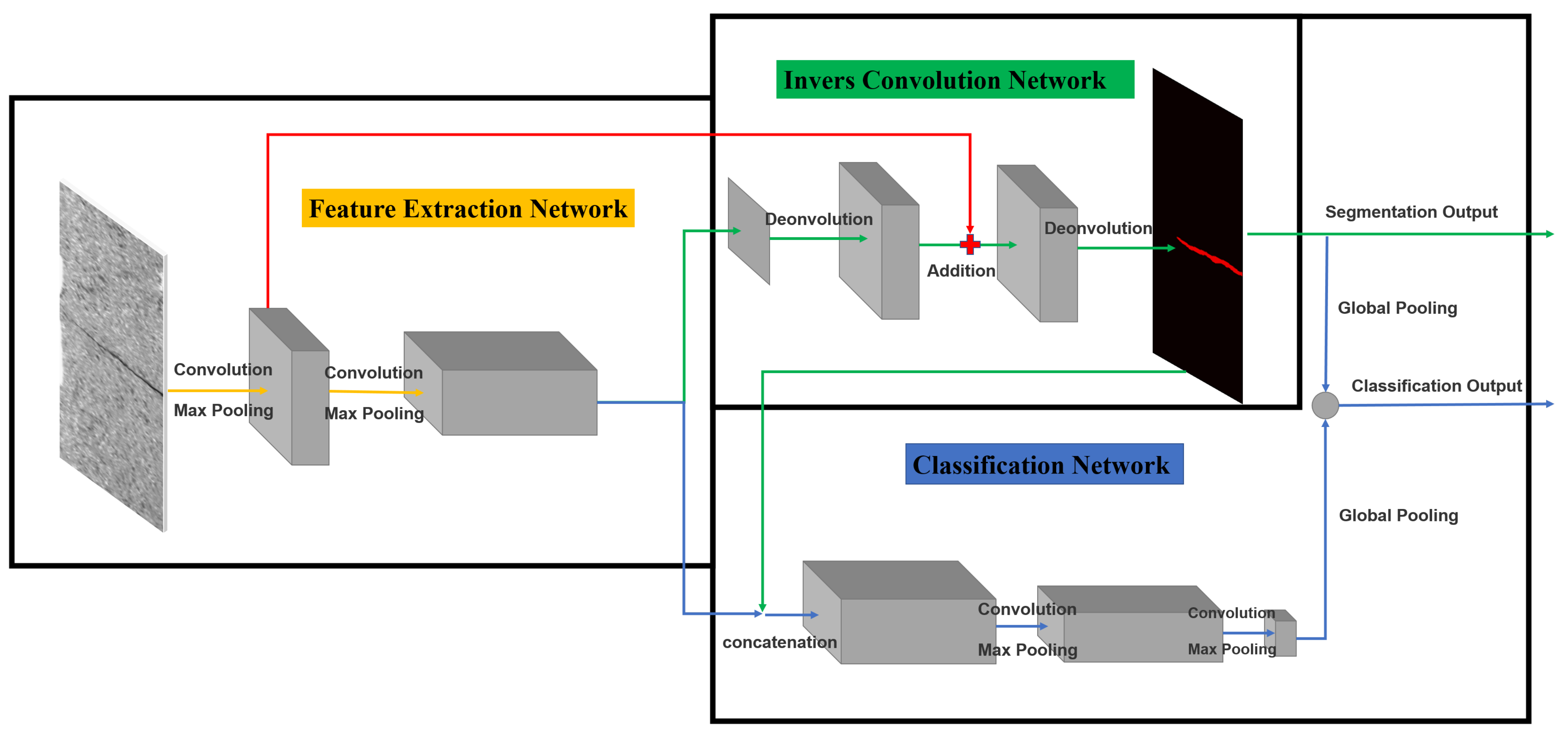
3.1. Network Framework

The framework of PSIC-Net is mainly divided into three parts as shown in Figure 2. The first part is the feature extraction network, which consists of 10 convolutional layers and 3 maximum pooling layers. After each convolutional layer, there is a batch normalization (BN) and a rectified linear unit (ReLU). The second part is the invers convolution network, which connects the last layer of the feature extraction network through a 1 × 1 convolution layer. It consists of 6 deconvolution layers (three of which are used for double up-sampling), 2 element-wise addition layers and 2 convolution layers. The third part is the classification network, which consists of 3 maximum pooling layers, 3 convolution layers, 4 global pooling layers and 1 full connection layer. The input of classification network concatenates the last layer of the feature extraction network and the output layer of the invers convolution network. Finally, it outputs the probability of defects.

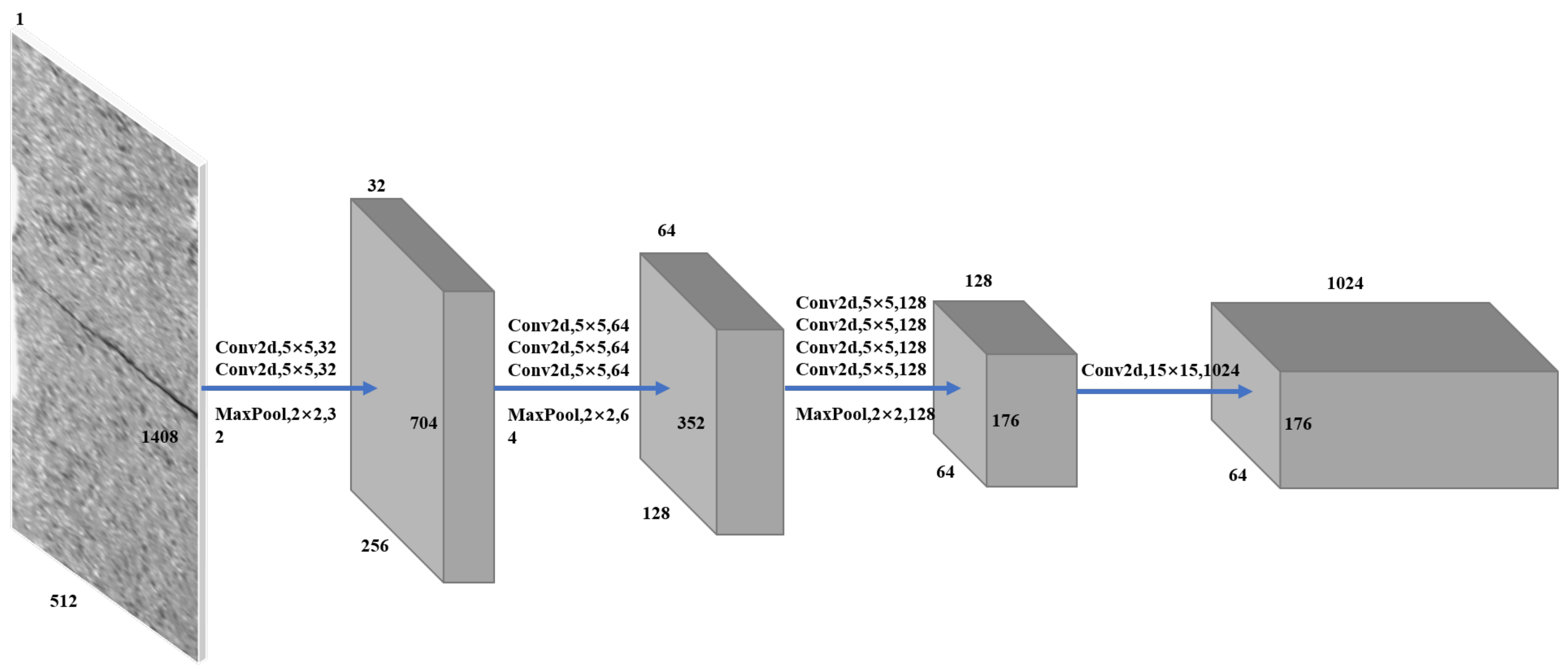
3.1.1. Feature Extraction Network

The feature extraction network is composed of 10 convolution layers and 3 maximum pooling layers. Each maximum pooling layer reduces the resolution of the image by two times, so the size of the final feature image is 1/8 of the original image. The first nine convolutional layers use 5 × 5 convolutional kernels, and the tenth layer uses the 15 × 15 convolutional kernel. Moreover, the first and second layers are set with 32 channels, the third to fifth layers with 64 channels, the sixth to ninth layers with 128 channels, and the tenth layer with 1024 channels. It can be seen that the convolutional network is set up in a gradually increasing number of layers and channels. This network structure can better extract the features of semantic information in the deep layers and still retain better spatial location features in the shallow layers, which is a win–win network setting mode for segmentation and classification. In addition, BN and Relu are connected after each convolutional layer to improve the convergence speed in the training process, make the model more stable, and prevent over-fitting and gradient disappearance [17]. Dropout is not used in this network since the weight sharing mechanism of the convolutional layer provides sufficient regularization. Because the number of defect samples is much smaller than the number of defect-free samples, not using dropout can prevent the small number of defect features and tiny defect features from being discarded. Figure 3 demonstrates the network structure. It should be noted that the size of the image in Figure 3 is just an example to show how the image size changes as the network deepens. The initial sizes of the images are not uniform, but have small size changes.

Feature extraction network is the key to the segmentation and classification of defects. Due to the scarcity of defect samples and the possibility that defects are minor, we increase the receptive field of the convolution layer in this part and retain all feature details as much as possible. To be specific, both the pooling operation and the large convolution kernel in the deep layer are designed to significantly increase the receptive field. The number of convolution layers between each maximum pooling layer increases successively, which can increase the capacity of features with the large receptive field. Finally, the selection of the maximum pooling layer, rather than other down-sampling methods, considers that the maximum pooling layer can retain small and important features [17].

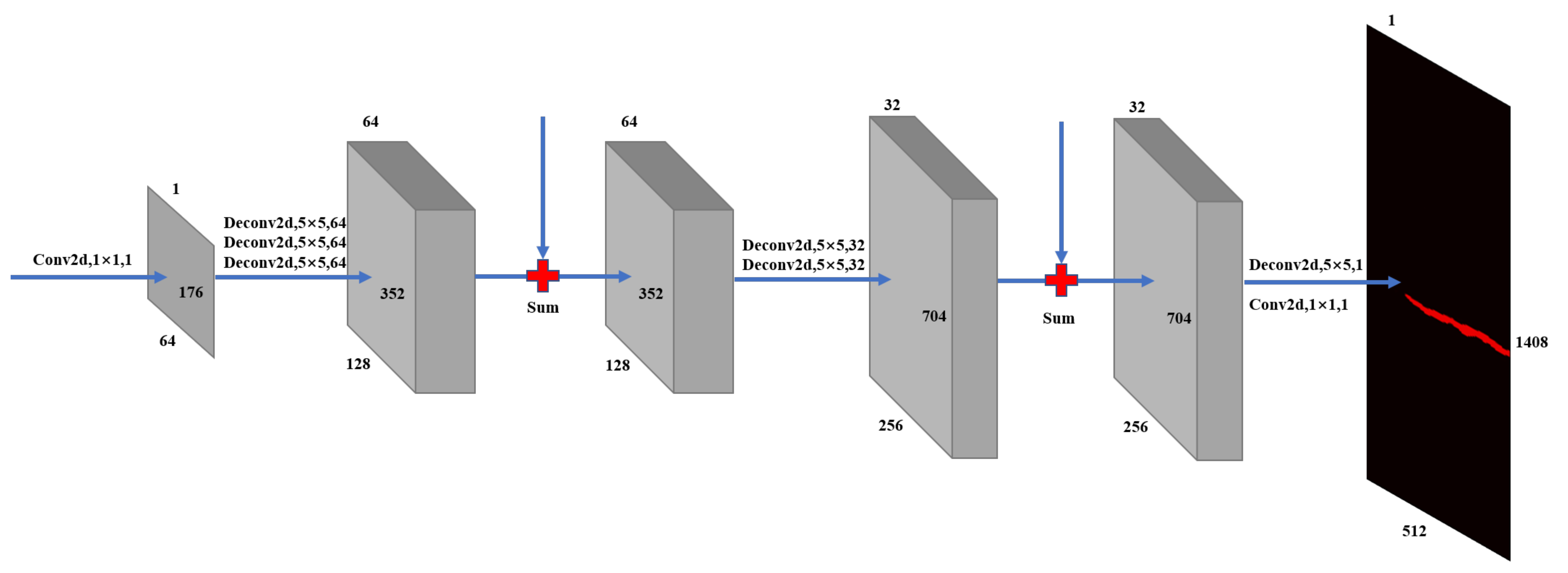
3.1.2. Invers Convolution Network

The invers convolution network consists of 6 deconvolutional layers, 2 element-wise addition layers and 2 convolution layers as shown in Figure 4. Among them, the first convolutional layer is used to integrate the features of the last layer of the feature extraction network to obtain a heatmap. The first $5\times 5$ deconvolutional layer with 64 channels is responsible for doubling the heatmap, so that the resolution of the heatmap becomes 1/4 of the raw image. Then, 2 deconvolutional layers with the same size and number of channels are connected (the deconvolutional layer does not magnify the resolution here). After that, the skip-layer structure [42] is introduced. That is, the feature map, which is downsampled twice in the feature extraction network (1/4 of the raw image), is added and fused with the heatmap that has the same shape here. This structure can re-introduce the features in the shallow layer so as to ensure the accuracy of the spatial position and the accuracy of the edge region segmentation. After that, the above structure is repeated once, but the difference is that the number of deconvolutional layers is reduced to 2 layers (here, the first layer of deconvolutional is still used for up-sampling, and the resolution of the heatmap is now 1/2 of the raw image), and the number of channels is reduced to 32. The feature map in the feature extraction network, which was pooled once, is added and fused with the heatmap here. Finally, the network is restored to the raw image size through 1-layer deconvolutional up-sampling. A single-channel $1\times 1$ convolutional layer is added to output the segmentation prediction graph.

The invers convolutional network is inspired by FCN [42] and DeconvNet [43] since they complete the segmentation task in a fairly effective way, which is especially critical for a model with a small number of sample data. Invers convolutional layers achieves the lifting of resolution, and element-wise addition layers fuse the feature map and heatmap. Both of them are conducive to the robustness and accuracy of the whole network.

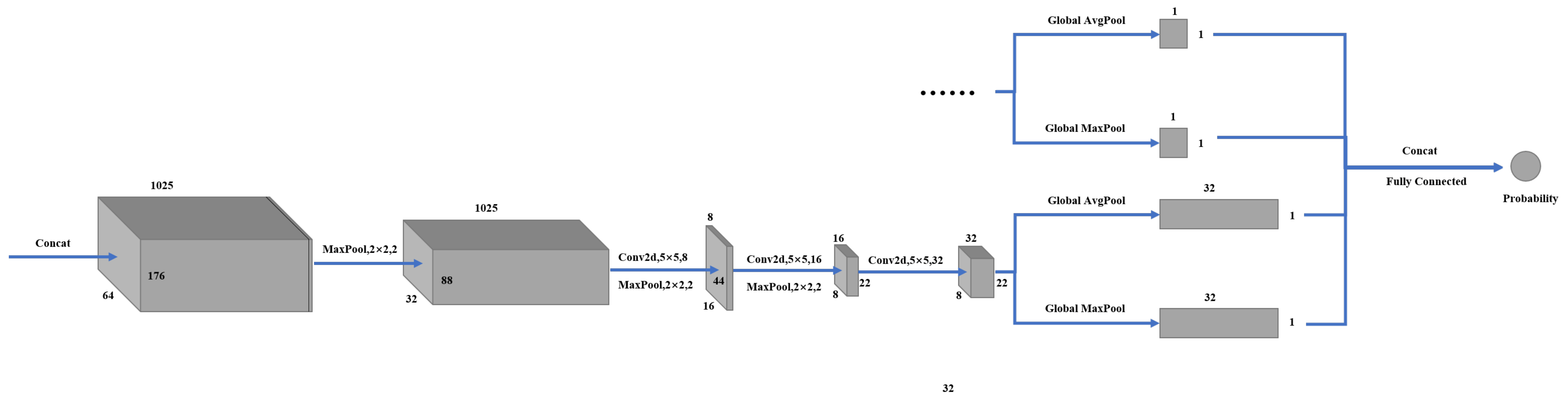
3.1.3. Classification Network

The design of the classification network refers to the classification network in [17] as shown in Figure 5. The classification network consists of 3 convolutional layers, 3 maximum pooling layers and 4 global pooling layers. The input concatenates the last layer of the feature extraction network and the output of the invers convolution network. The number of channels of the convolutional layer increases as the image resolution decreases, which can balance the computing cost of each layer. After three rounds of convolution and pooling, the network connects one global maximum pooling layer and one global average pooling layer, respectively, to reduce the parameters and integrate features, and finally obtains two $32\times 1$ feature vectors. In order to further improve the accuracy of the classification results, the output of the invers convolution network is also connected to one global maximum pooling layer and one global average pooling layer, respectively, to obtain two $1\times 1$ feature vectors. Because the global pooling layers output a one-dimensional vector for each channel, it can eliminate the dimension mismatch between the invers convolutional network and the classification network. Finally, a fully connected layer is used to concatenate the feature vectors as the output. The output is the probability of whether the image contains defects.

After using the last layer of the feature extraction network as input, the classification network still carries out three rounds of convolutional and down-sampling operations to ensure that the overall defect features can be completely retained. The output of the invers convolutional network is introduced to prevent the classification network from over-fitting. In the training process, the classification network and invers convolutional network are adversarial and fuse with each other, making the final classification result more accurate.

3.2. Training

Since the whole network is composed of a relatively independent segmentation network (feature extraction network and invers convolutional network are collectively called the segmentation network) and classification network, a two-step training mode of the two networks is proposed, which allows the parameters of the two networks to be trained, according to the different tasks (segmentation or classification). The two-step training mode can reduce the interference and influences between the two networks to the minimum. In fact, the end-to-end training mode is also considered. Bozic et al. [36] propose a total loss function as shown in Equation (1).

$${\mathcal{L}}_{total}=\lambda ·{\mathcal{L}}_{seg}+\delta ·(1-\lambda )·{\mathcal{L}}_{cls}$$

(1)

where ${\mathcal{L}}_{seg}$ and ${\mathcal{L}}_{cls}$ represent segmentation loss and classification loss, respectively, $\delta$ is an additional classification loss weight to prevent the classification loss from dominating the total loss, and $\lambda$ is a mixed factor which is limited by the super parameter: epoch. It can balance the contribution of each network in the final loss too.

The experiment in this paper tests this training mode. The results demonstrate that the training time is indeed shortened, but the output results, especially the segmentation results, are not comparable to the two-step training mode. The primary analysis is that the weight parameters of each part may be balanced, due to the restraint of the two networks in the end-to-end training mode, which not only increases the difficulty of network convergence, but also affects the implementation of the two networks and fails to achieve any benefits. Therefore, the final training mode is determined to train the segmentation network first, then freeze the feature extraction network and invers convolutional network parameters, and finally train the classification network and perform the fine-tuning. This training mode can avoid parameter weights over-fitting the invers convolutional network or the classification network, improving the accuracy of both the segmentation and classification.

The problem of sample imbalance exists in both the segmentation and classification of PSIC-Net. There are fewer positive samples (defective samples) and much more negative samples (non-defective samples). If the positive and negative samples are multiplied by the same weight coefficient, it is easy to predict the positive samples into negative samples. Therefore, this paper introduces the weighted cross-entropy loss function [44,45]. Assigning a larger penalty weight to the classification errors of positive samples and multiplying the classification errors of negative samples by a smaller weight can improve the accuracy of both segmentation and classification. In addition, since the mechanism of the segmentation network is to classify every pixel, the weighted cross-entropy function can also improve the segmentation accuracy of small defects and the boundary. In industry, the influence of false negative cases is much greater than that of false positive cases, which is another reason why we introduce weighted cross-entropy loss. The weighted cross-entropy loss function adopted in this paper is shown in Equation (2).

$${\mathcal{L}}_{WCE}=-\alpha \sum _{j\in X_{+}}logPr(x_j=1)-(1-\alpha )\sum _{j\in X_{-}}logPr(x_j=0)$$

(2)

where ${\mathcal{L}}_{WCE}$ denotes the weighted cross-entropy loss function. The loss function is computed over all pixels in the training image $X=(x_j,j=1,\dots ,|X\left|\right)$. $\alpha$ is the class-balancing factor on a per-pixel term basis. $\alpha =|X_{-}|/|X|$ and $1-\alpha =|X_{+}|/|X|$. $X_{-}$ and $X_{+}$ denote the defect-free and defect ground truth label pixels, respectively.

3.3. Inference

Once PSIC-Net is trained, images can be input for inference. The input image can be of any size since the full connected layer of the classification network is obtained after global pooling. There is no dimension-matching problem. In order to verify the universality of the network to all kinds of surface-defect data, the public defect datasets used for training and test in this paper are KolektorSDD [17], KolektorSDD2 [18] and DAGM [19].

The inference results of PSIC-Net have two outputs, namely, the defect segmentation and the image classification. The first output is the pixel-wise segmentation output by the invers convolutional network, which is a mask image obtained by probability. The size of the output image is the same as that of the raw image. The defect and the background will be distinguished by different colors, as shown in Figure 6.

The second output is the probability, which represents whether there is a defect in the image inferred by the classification network.

4. Experiments and Results

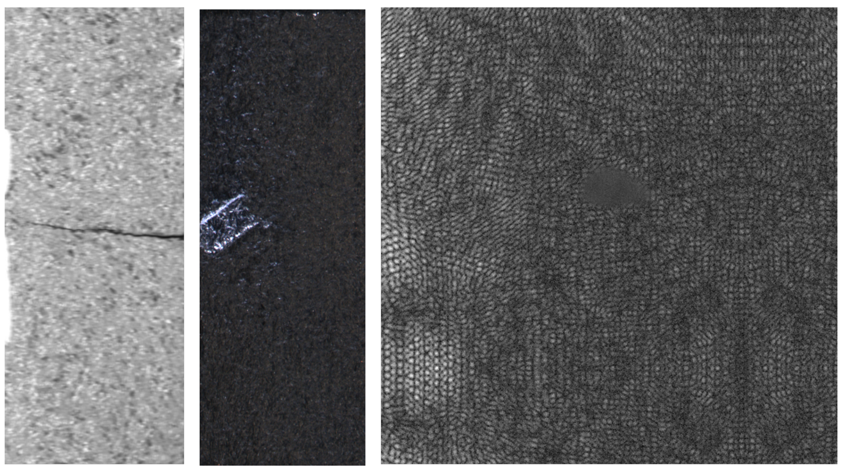
4.1. Datasets

KolektorSDD [17] is constructed from images of defective production items that were provided and annotated by Kolektor Group d.o.o. The images were captured in a controlled industrial environment in a real-world case. The dataset consists of 399 images, including 52 images with visible defects and 347 images without any defect. The images in this dataset are not uniform in size, but have small size changes. The sizes of the images are about 512 pixels in width and about 1408 pixels in height. There is only one defect in the image with defect. The remaining 347 images serve as negative examples with non-defective surfaces. As shown in Figure 7.

KolektorSDD2 [18] dataset is constructed from images of defected production items that were provided and annotated by Kolektor Group d.o.o. Various types of defects were observed on the surface of the item. The images were captured in a controlled industrial environment. The dataset consists of 356 images with visible defects and 2979 images without any defect. The image sizes are approximately 230 × 640 pixels. Below are four examples as shown in Figure 8.

DAGM [19] is regarded as one of the most widely recognized public surface defect datasets, which contains 10 classes of defect images. Each class of images contains about 1000 images, and a small part of each class of image has a random defect generated by the computer. The backgrounds of the images in the same class are quite similar, but those of different classes are diverse. Each image is 512 × 512 pixels in size. The label for this dataset is a weakly supervised label, that is, the defective areas are represented by an ellipse mask. Figure 9 demonstrates four examples.

4.2. Experiment Settings

PSIC-Net can carry out independent experiment without the need for pre-training on other datasets. The network is randomly initialized, using standard normal distribution and adopts momentum-free stochastic gradient descent for training. Moreover, the initial learning rate is set reasonably, and the learning rate decreases dynamically with gradient descent. Four 1080Ti GPUs are used for both training and inference. In addition, the experiment adopts the triple cross-validation method, which means that images in each dataset are randomly assigned for the training sets and the test sets three times. During the training, three training sets are trained in sequence, and three corresponding test sets are also tested in turn.

The experiment is implemented on Tensorflow 1.12, Python 3.5, CUDA 9.0.

4.3. Performance Metrics

We evaluate the performance of PSIC-Net in three public datasets, using the triple cross-validation method. Intersection over Union (IoU) is generally used to measure the accuracy of segmentation. It means the ratio of intersection and union of predicted mask and ground truth mask. In our study, Mask IoU and Boundary IoU [46] are used to measure the defect segmentation effect of PSIC-Net. Boundary IoU is a sensitive measurement method for the quality of boundary segmentation. Their calculation formulas are displayed in Equations (3) and (4) respectively.

$$MaskIoU(G,P)=\frac{|G\cap P|}{|G\cup P|}$$

(3)

$$BoundaryIoU(G,P)=\frac{|(G_d\cap G)\cap (P_d\cap P)|}{|(G_d\cap G)\cup (P_d\cap P)|}$$

(4)

where G and P denote ground truth and prediction of the mask image. $G_d$ denotes pixels within the distance of d from the boundary of ground truth mask. Similarly, $P_d$ denotes pixels within the distance of d from the boundary of the prediction mask.

The performance metrics used to measure the effect of classification are area under ROC curve (AUC), average precision (AP) and accuracy. To be specific, AUC represents the area between receiver operating characteristic curve (ROC) and the horizontal axis. AUC can intuitively evaluate the quality of the classifier, and the larger the value is, the better the model is. Average precision (AP) is the area between the precision–recall curve (PR) and the horizontal axis. As a recognized metrics, AP has the advantage of measuring the effectiveness of a model on highly unbalanced datasets. In addition, the mean average precision (mAP) in this paper represents the mean value of AP of each test set.

4.4. Experiment Results

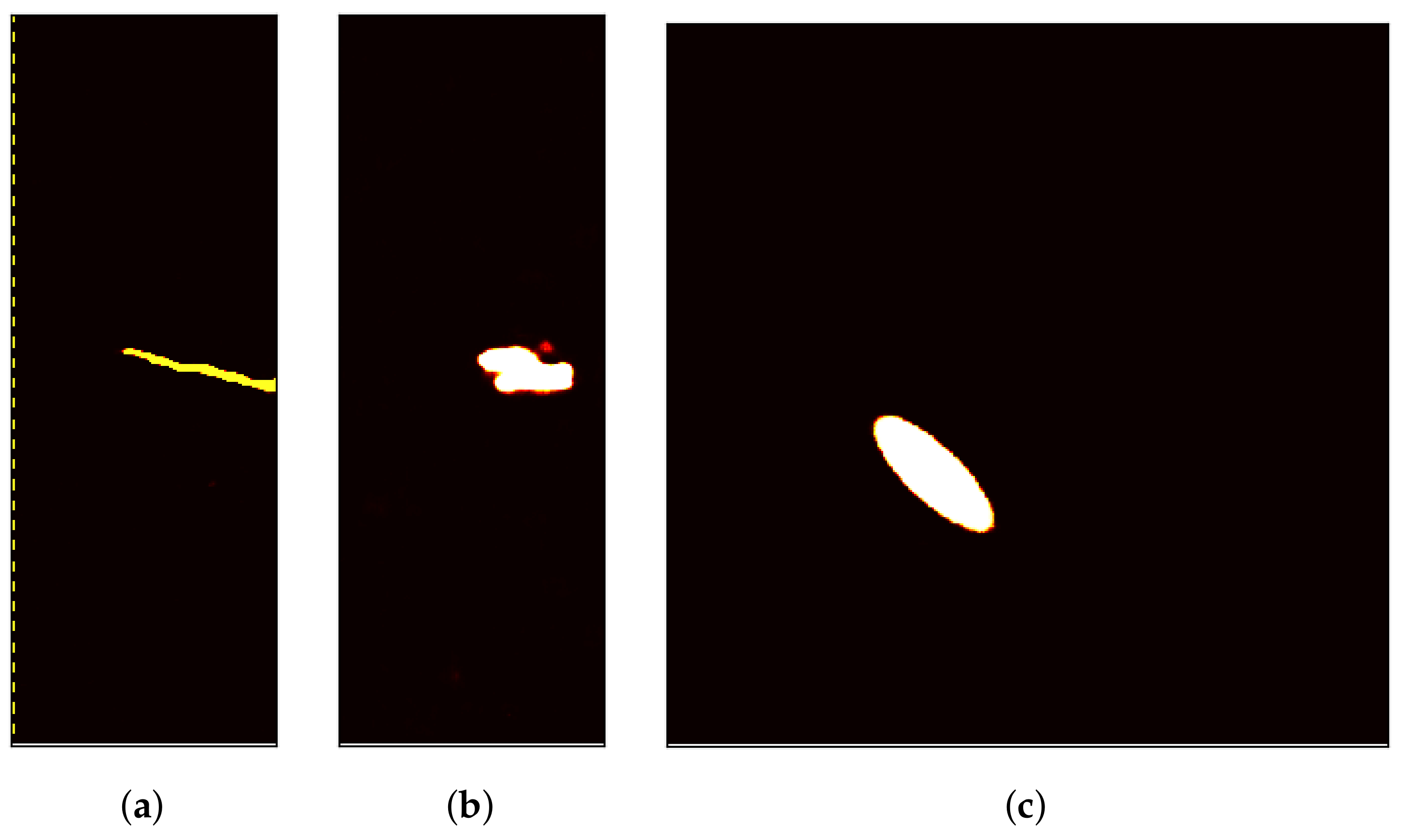
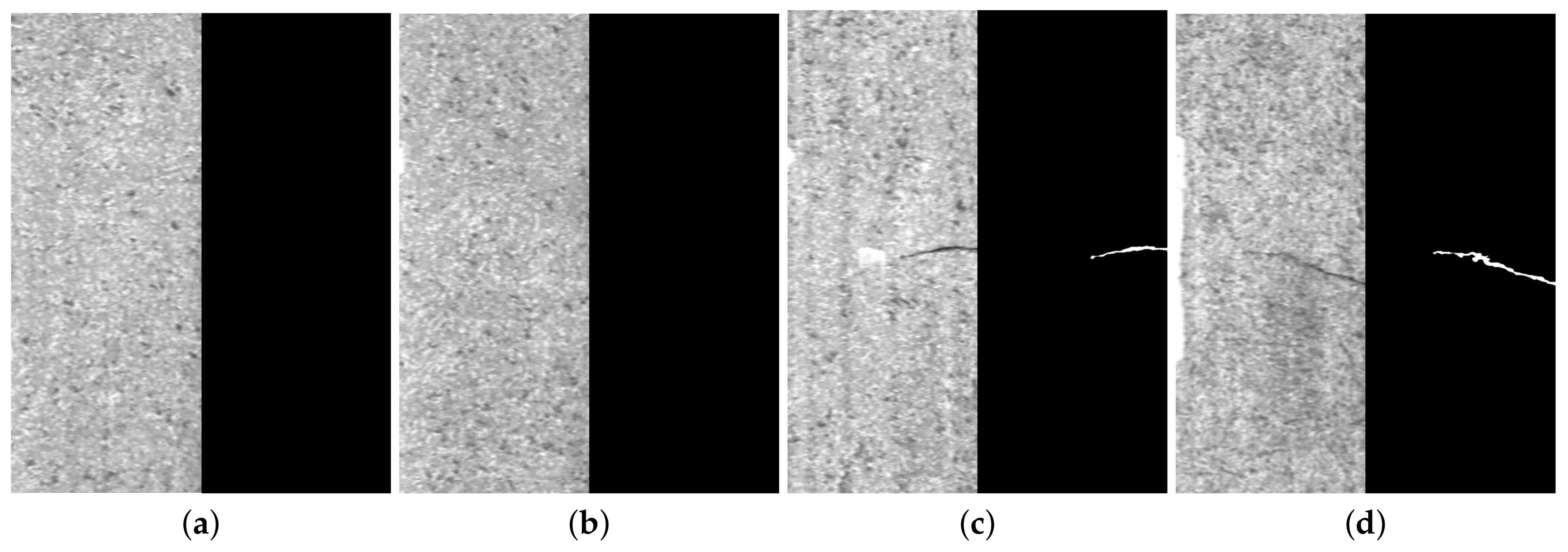
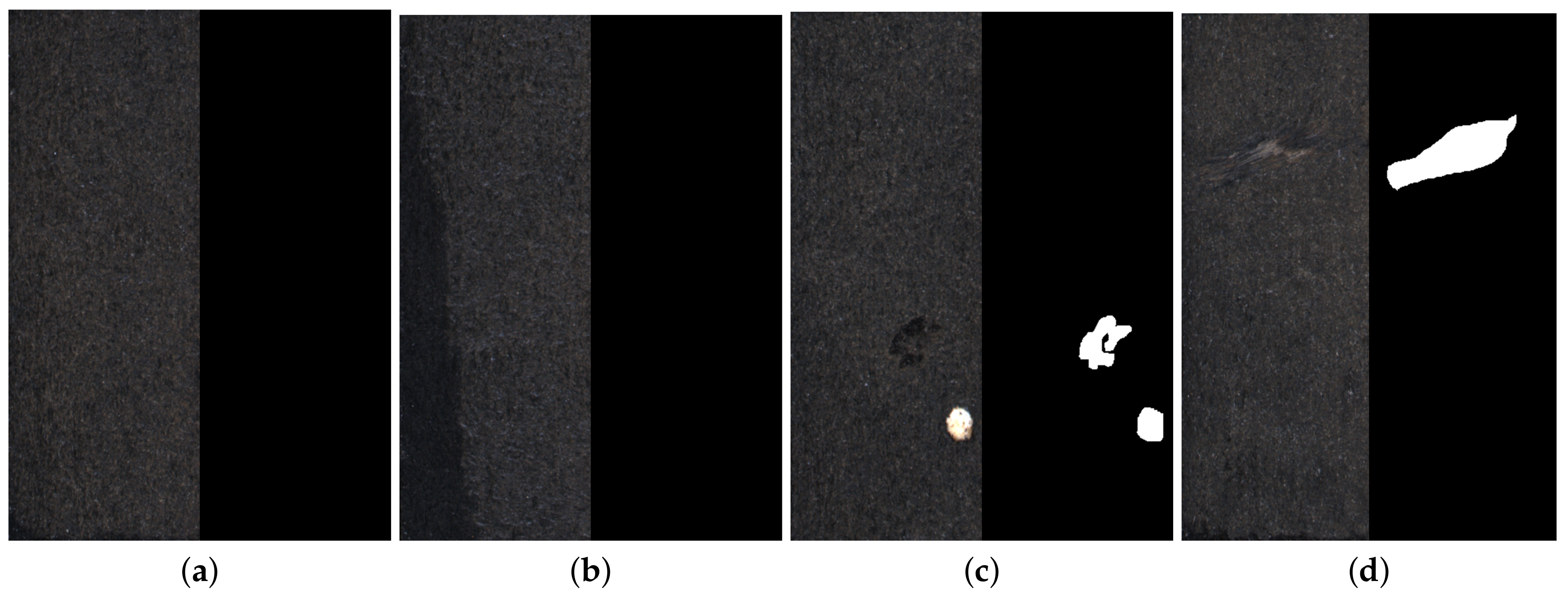
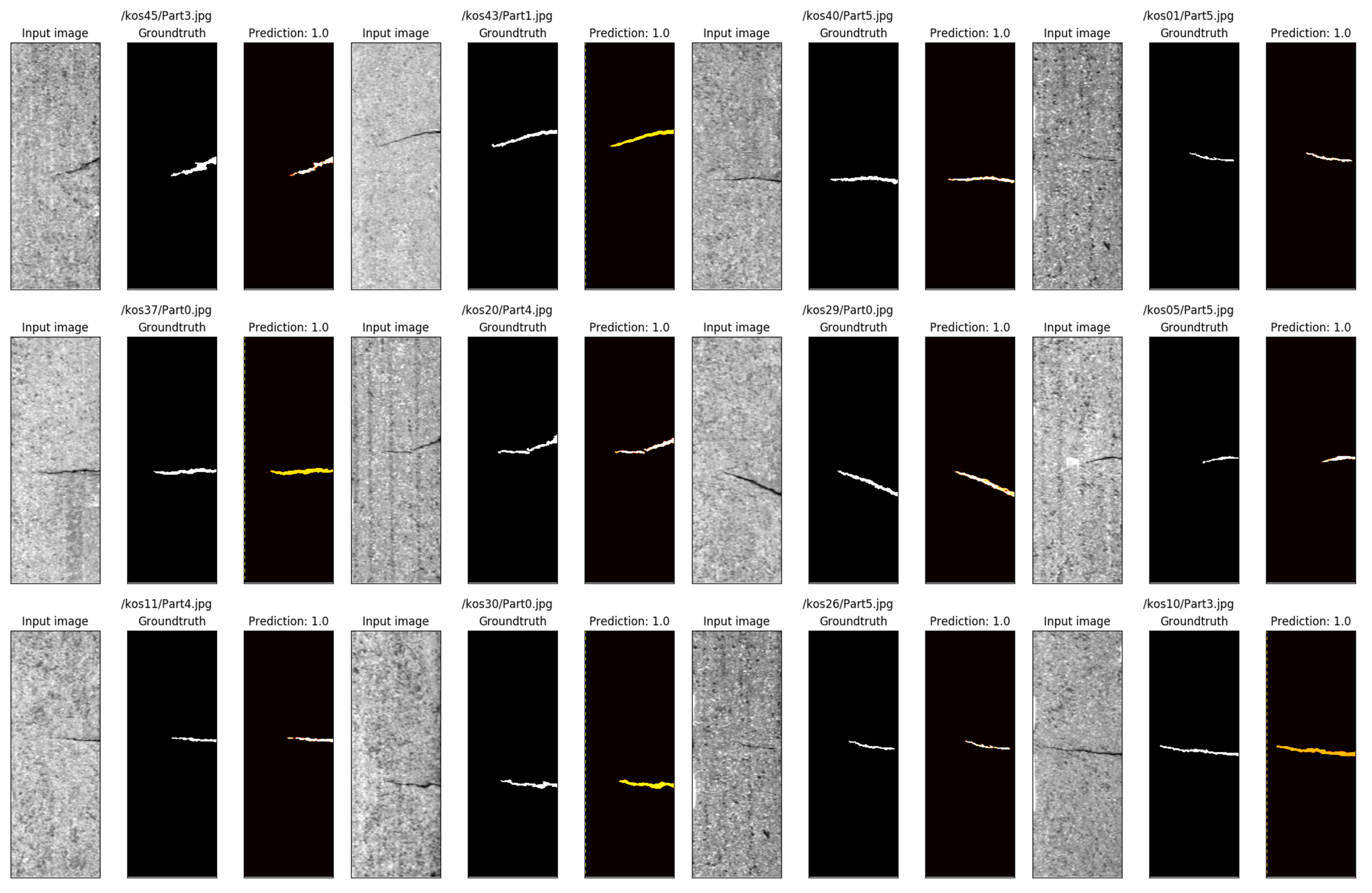
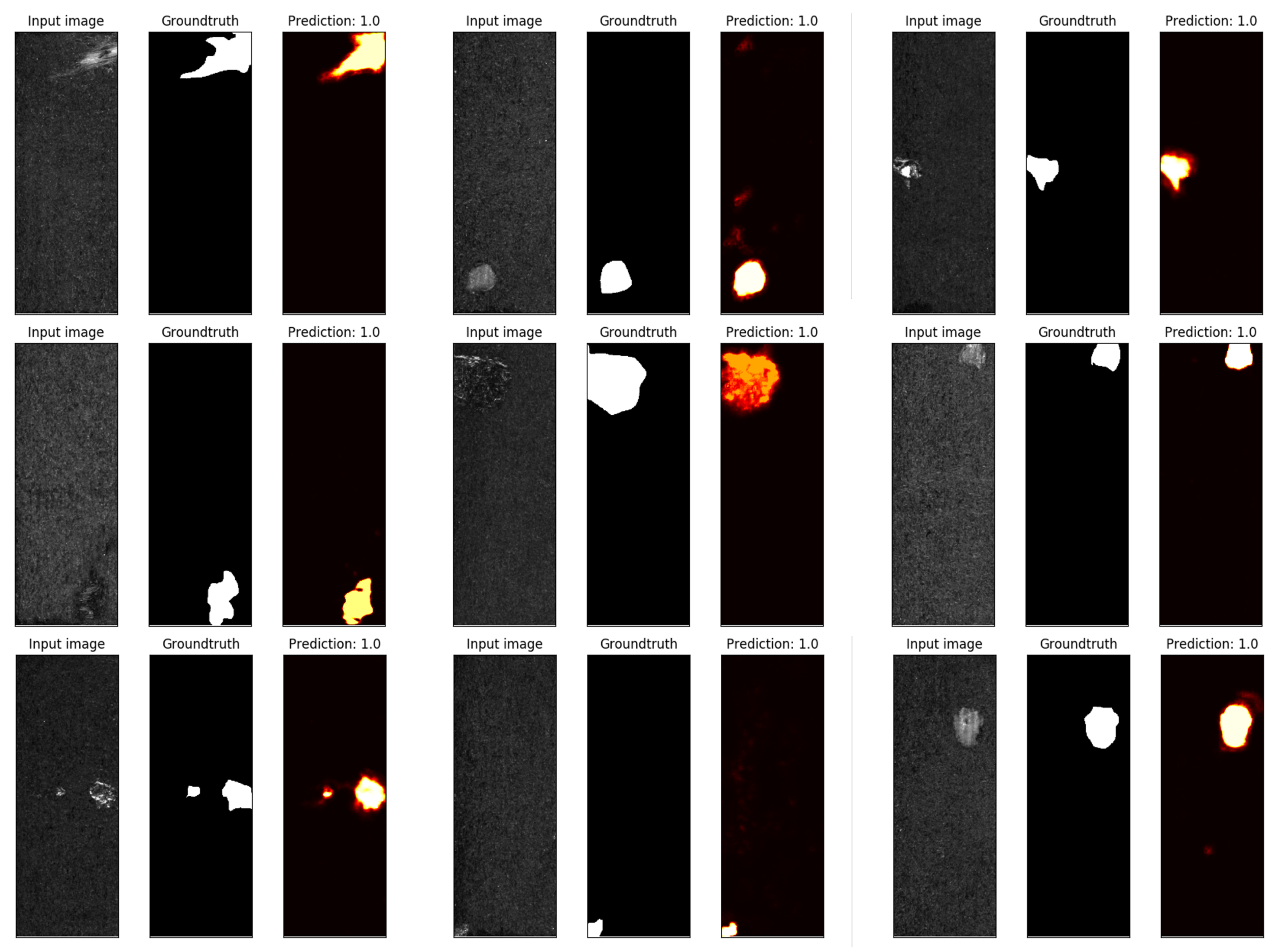
4.4.1. Experiment Results of Defect Segmentation

Firstly, the defect segmentation results are introduced. Figure 10, Figure 11 and Figure 12 respectively demonstrate some typical defect segmentation results of KolektorSDD, KolektorSDD2, and DAGM.

Figure 10, Figure 11 and Figure 12 intuitively demonstrate that the segmentation network of the model can perform defect segmentation well under the condition of different defect types, shapes and sizes. The model is able to not only accurately segment defects, but also predict the shapes of the defects that are basically the same as labels.

In order to further analyze the segmentation results, we sort out all predicted output images of defect segmentation, and find corresponding ground truth images. According to the calculation of mask IoU and boundary IoU, all defect segmentation images are tested, and the results are demonstrated in

Table 1. Defect segmentation results of PSIC-Net.

Datasets	Mask mIoU (%)	Max Mask IoU (%)	Min Mask IoU (%)	Boundary mIoU (%)	Max Boundary IoU (%)	Min Boundary IoU (%)
KolektorSDD	88.49	89.25	86.88	73.99	80.63	69.46
KolektorSDD2	86.13	87.79	83.05	70.98	73.99	65.98
DAGM	89.10	89.93	87.01	82.55	88.21	77.56

.

According to Table 1, the mask mIoU of KolektorSDD reaches 88.49% and boundary mIoU 73.99%. The mask mIoU of KolektorSDD2 reaches 86.13% and boundary mIoU reaches 70.98%. The mask mIoU of DAGM reaches 89.10% and boundary mIoU reaches 82.55%. On the whole, PSIC-Net achieves a good segmentation effect in various datasets, especially in DAGM. This is because DAGM is a weakly-labeled dataset, all defects are artificially generated ellipse defects, PSIC-Net is quite effective for this simple defect segmentation. The mask IoU of KolektorSDD and KolektorSDD2 reduces slightly compared to that of DAGM. The reason is that KolektorSDD and KolektorSDD2 come from real industry, so the defects are much more complex. So the difficulty of segmentation is, thus, upgraded. Moreover, the boundary IoU decreases more. The reason is that the boundary of defects in real industry are usually uneven. When segmenting this dataset, PSIC-Net needs to process more complex edge pixel segmentation, resulting in the decrease in boundary IoU.

In order to further verify the segmentation effect of PSIC-Net, we compare the segmentation effect of several great defect segmentation methods with that of PSIC-Net, as shown in

Table 2. Comparison of segmentation effects of various methods and PSIC-Net.

Methods	Datasets	Mask mIoU (%)	Boundary mIoU (%)
FCN [42]	DAGM	73.86	-
DeepLab [47]	DAGM	74.61	-
[27]	DAGM	84.50	-
[48]	DAGM	73.56	-
[31]	DAGM	74.78	-
[18,36]	KolektorSDD	76.21	-
	KolektorSDD2	71.69	-
	DAGM	79.46	-
[17]	KolektorSDD	87.77	71.23
	KolektorSDD2	84.20	63.59
	DAGM	87.79	77.13
PSIC-Net(ours)	KolektorSDD	88.49	73.99
	KolektorSDD2	86.13	70.98
	DAGM	89.10	82.55

.

It can be seen from the data in Table 2 that both mask IoU and boundary IoU are ahead of other methods, especially in the performance of DAGM, which exceeds 15.54% at most. Compared with [17], which has relatively good segmentation results, PSIC-Net also has a small advantage. This proves that PSIC-Net is effective in defect segmentation.

4.4.2. Experiment Results of Defect Image Classification

Table 3. The results of PSIC-Net in defect image classification.

Datasets	AUC (%)	mAP (%)	Accuracy (%)
KolektorSDD	98.05	96.43	98.53
KolektorSDD2	96.34	93.27	97.50
DAGM	100	100	100

shows the results of PSIC-Net in defect image classification.

As can be seen from Table 3, PSIC-Net performs well in classification, especially in the DAGM, where the classification accuracy can reach 100%. The mAP of KolektorSDD2 can also reach 93.27%. The overall classification accuracy is positively correlated with the complexity of the dataset. After analyzing the misclassified false positive (FP) images, we find that most FP are caused by missing labels in the ground truth of the dataset. As shown in Figure 13, KolektorSDD only considers significant scratches when labeling defects, but tiny defects may be omitted. In KolektorSDD2, there are also some cases, where small color difference patches and small scratches are not labeled, as shown in Figure 14. In fact, the appearance of these FP images also shows the strong segmentation and classification ability of PSIC-Net. The false negative (FN) images in KolektorSDD2 are misjudged since the defects are too obscure, as shown in Figure 15. It is worth mentioning that PSIC-Net actually assigns a small probability to the defects of the segmentation images in Figure 15, but the classification network finally determines it as being defect-free. The tradeoffs here are worth studying in the future.

To further verify the performance of PSIC-Net, we compare it with several defect classification methods, as shown in

Table 4. Comparison of classification effects of various methods and PSIC-Net.

Methods	Datasets	AUC (%)	mAP (%)	Accuracy (%)
[49]	DAGM	-	-	99.90
[50]	DAGM	99.60	-	99.40
[19]	DAGM	-	-	99.20
[51]	DAGM	99.00	-	99.80
[23]	DAGM	-	-	99.40
[52]	DAGM	-	-	99.80
[53]	DAGM	-	-	99.90
[54]	KolektorSDD	-	98.80	-
[55]	KolektorSDD	-	100	-
[36]	KolektorSDD	-	97.36	98.12
	DAGM	-	100	100
[18]	KolektorSDD	-	97.36	98.12
	KolektorSDD2	-	95.40	-
	DAGM	-	100	100
[17]	KolektorSDD	88.49	89.24	87.41
	KolektorSDD2	83.86	68.65	86.67
	DAGM	100	100	100
PSIC-Net(ours)	KolektorSDD	98.05	96.43	98.53
	KolektorSDD2	96.34	93.27	97.50
	DAGM	100	100	100

.

As can be seen from the data in Table 4, the classification performance of PSIC-Net on each dataset is good. In DAGM, the three performance metrics have reached 100%, which is consistent with the studies of [17,18,36]. In KolektorSDD and KolektorSDD2, the metrics of PSIC-Net decreased slightly. As mentioned earlier, the false classification basically comes from the missing labeling of defects. The designs presented in studies [17,18,36] were reproduced, and the data about them in Table 4 are the real measured data. In KolektorSDD, the AUC and accuracy are the highest in PSIC-Net. The mAP of the study [55] is the highest, reaching 100%. However, due to the missing labeling in KolektorSDD, we have reason to suspect that the study [55] does not use the missing labeling data. As we are unable to reproduce this paper, we have reservations about the result of it for the time being. Compared with other methods, PSIC-Net still has certain advantages. Similarly, in KolektorSDD2, the mAP of PSIC-Net is almost consistent with that of the study [18].

4.4.3. Time Cost of Training and Inference

Firstly, the clock synchronization function is used to synchronize the clock of software and hardware. Then, we set the timing starting point before the input and the timing ending point after the output of both the training and inference. Finally, the time cost can be calculated by the timing ending point minus the timing starting point. Four 1080Ti GPUs are executed in parallel to lift the speed.

The average training time of the segmentation network with the training set of KolektorSDD is 68 min; the average training time of the classification network is 23 min; and the average inference time of a single image is 1.03 s (a total of 264 images are used in each training, and the size of a single image is about 1408 × 512 pixels). The average training time of the segmentation network with KolektorSDD2 is 27 min; the average training time of the classification network is 20 min; and the average inference time of a single image is 0.7 s (a total of 334 images are used in each training, and the size of a single image is about 640 × 230 pixels). The average training time of segmentation network with DAGM is 31 minutes; the average training time of classification network is 24 min; and the average reasoning time of single image is 0.95 s (a total of 575 images are used in each training, and the size of a single image is about 512 × 512 pixels).

In the actual industry, the defect detection time of a product is about 1–2 s. It can be seen that the inference time of PSIC-Net has reached the detection time required by the actual industry, and can complete the online detection task.

5. Discussion

Extensive experiments have proved that PSIC-Net has a significant result on the classification and segmentation of surface defects. Through the design of the network, the selection of the training mode and the improvement of the loss function, the PSIC-Net can acquire features from a small number of sample data, and can classify and segment the defect quickly and accurately. At the academic level, PSIC-Net has achieved state-of-the-art classification and segmentation. In the intelligent manufacturing scenario, PSIC-Net can also provide some practical ideas for defect detection.

Generally, in actual industrial production, it is only necessary to know whether the product is defective. However, people need to segment defects when they study the causes of defects or specific defect features. The two networks address different problems. Because the three sub networks are relatively independent, the segmentation network and classification network have the ability to operate independently. The reasons why we propose the classification network are as follows. Firstly, whether training or inference, the speed of the classification network is much faster than that of the segmentation network. This is because the defect segmentation is, essentially, to classify each pixel, which will take a long time to classify the pixels of the whole image. We can disable the output of segmentation network when some tasks that require faster detection speed are accepted. Secondly, only from the accuracy of classification, the effect of the classification network is much better than that of the segmentation network. The segmentation network classifies each pixel, which will lose many defective spatial and overall features, resulting in the decline of the classification accuracy. However, the classification network is continuously refined from the overall features of the image, which can better extract the features of defects and improve the accuracy. This is why most of the existing defect detection applications use defect classification rather than defect segmentation, which contains more information.

PSIC-Net still has some topics that need to be improved and studied in depth:

• The network is sensitive to data, and the results may fluctuate slightly even if the data remain unchanged. Making the network more stable during training is needed.
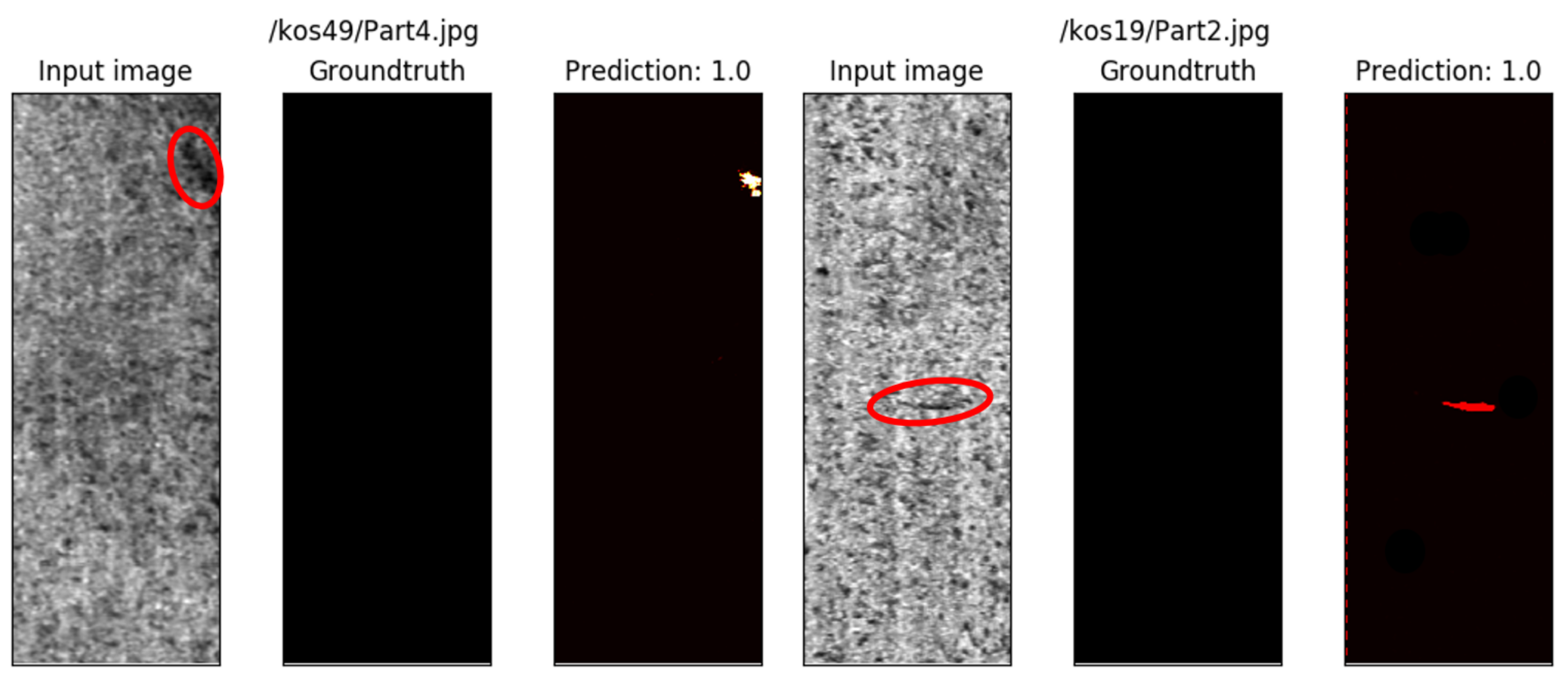
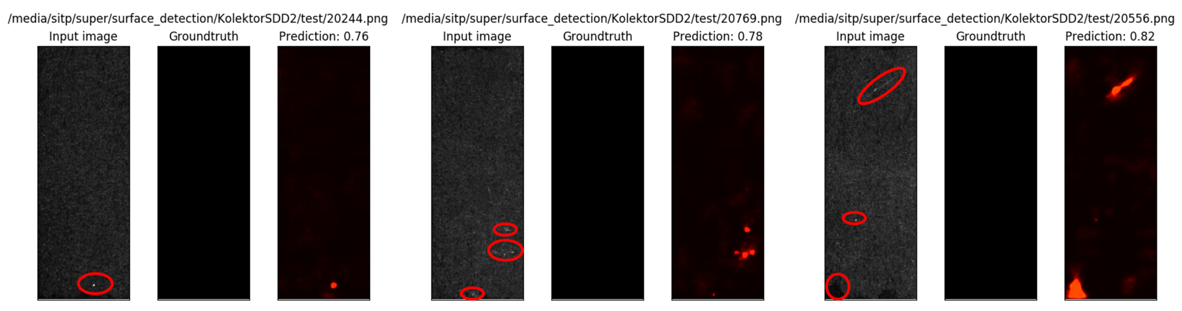
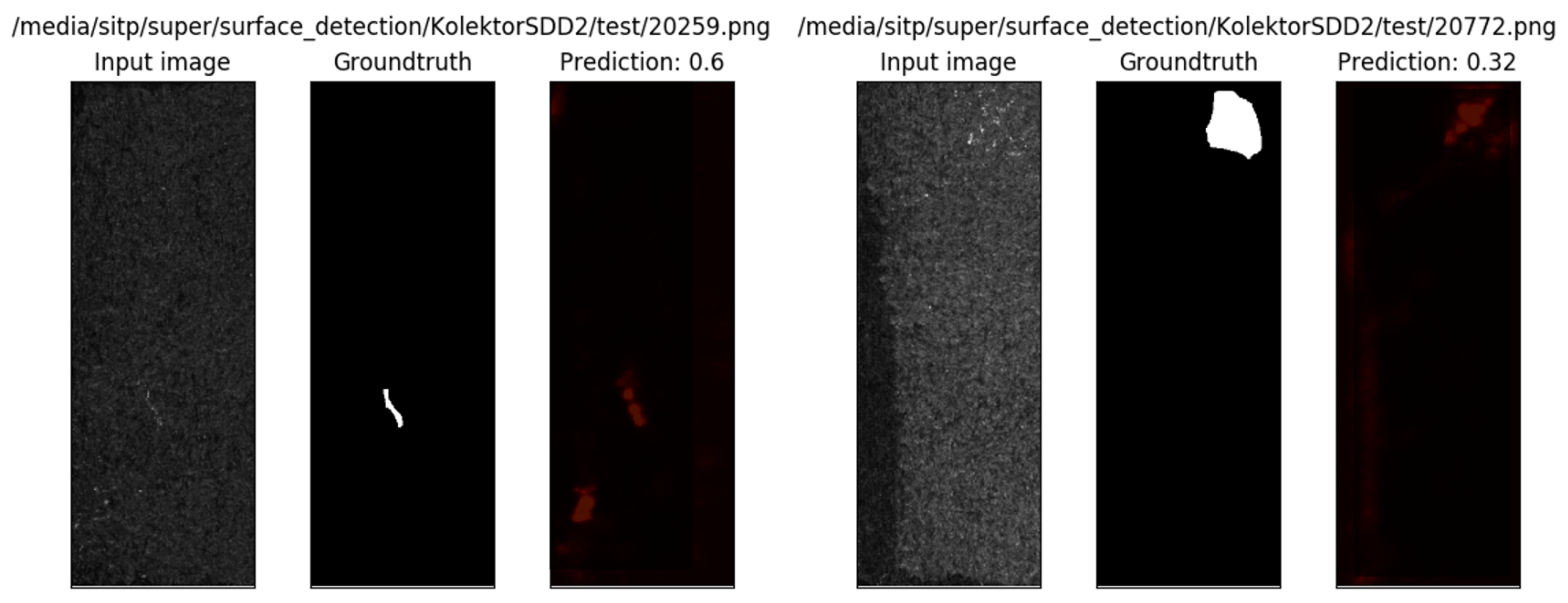
• The guidance of the segmentation network results to the classification network needs to be improved. In the experiment, it is found that a small number of defect data successfully segmented by the segmentation network are not successfully classified by the classification network. Strengthening the synergy of the two networks to improve the accuracy of the classification network also needs to be further explored.

6. Conclusions

This paper proposes a novel surface defect classification and segmentation network: pixel-wise segmentation and image-wise classification network, which consists of a three-stage architecture of feature extraction network, invers convolution network and classification network. This network can classify the surface defect images and segment the defects at the pixel level, and obtain the two outputs simultaneously. The advantage of PSIC-Net is that it can acquire key features from a small number of defective training samples. Moreover, by improving the loss function, this network can solve the problem of the poor training effect caused by the imbalance of positive and negative samples. By training the segmentation network and classification network step by step, high segmentation accuracy and classification accuracy can be obtained simultaneously. The validation and comparison experiments were carried out on three public datasets, and the experimental results of both classification and segmentation are satisfactory.

References

1. Guo, X.; Tang, C.; Zhang, H.; Chang, Z. Automatic thresholding for defect detection. ICIC Express Lett. 2012, 6, 159–164. [Google Scholar]
2. Oliveira, H.; Correia, P.L. Automatic Road Crack Segmentation Using Entropy and Image Dynamic Thresholding. In Proceedings of the 2009 17th European Signal Processing Conference, Scotland, UK, 24–28 August 2009. [Google Scholar]
3. Jia, C.; Wang, Y. Edge detection of crack defect based on wavelet multi-scale multiplication. Comput. Eng. Appl. 2011, 47, 219–221. [Google Scholar]
4. Xi, Y.; Qi, D.; Li, X. Multi-scale Edge Detection of Wood Defect Images Based on the Dyadic Wavelet Transform. In Proceedings of the International Conference on Machine Vision & Human-Machine Interface, Kaifeng, China, 24–25 April 2010. [Google Scholar]
5. Kanopoulos, N.; Vasanthavada, N.; Baker, R.L. Design of an image edge detection filter using the Sobel operator. IEEE J. Solid-State Circuits 1988, 23, 358–367. [Google Scholar] [CrossRef]
6. Li, E.S.; Zhu, S.L.; Zhu, B.S.; Zhao, Y.; Song, L.H. An Adaptive Edge-Detection Method Based on the Canny Operator. In Proceedings of the International Conference on Environmental Science & Information Application Technology, Wuhan, China, 4–5 July 2009. [Google Scholar]
7. Wang, D.; Zhou, S.S. Color Image Recognition Method Based on the Prewitt Operator. In Proceedings of the International Conference on Computer Science & Software Engineering, Wuhan, China, 19–20 December 2009; pp. 170–173. [Google Scholar]
8. Ojala, T.; Pietikainen, M.; Maenpaa, T. Multiresolution Gray-Scale and Rotation Invariant Texture Classification with Local Binary Patterns. IEEE Trans. Pattern Anal. Mach. Intell. 2002, 24, 971–987. [Google Scholar] [CrossRef]
9. Lei, L.J.; Sun, S.L.; Xiang, Y.K.; Zhang, Y.; Liu, H.K. bottleneck issues of computer vision in intelligent manufacturing. J. Image Graph. 2020, 25, 1330–1343. [Google Scholar]
10. Cortes, C.; Vapnik, V. Support-Vector Networks. Mach. Learn. 1995, 20, 273–297. [Google Scholar] [CrossRef]
11. Jeon, Y.J.; Choi, D.c.; Yun, J.P.; Park, C.; Kim, S.W. Detection of scratch defects on slab surface. In Proceedings of the 2011 11th International Conference on Control, Automation and Systems, Gyeonggi, Korea, 26–29 October 2011; pp. 1274–1278. [Google Scholar]
12. Neogi, N.; Mohanta, D.K.; Dutta, P.K. Review of vision-based steel surface inspection systems. EURASIP J. Image Video Process. 2014, 2014, 1–19. [Google Scholar] [CrossRef] [Green Version]
13. Bhatt, P.M.; Malhan, R.K.; Rajendran, P.; Shah, B.C.; Gupta, S.K. Image-Based Surface Defect Detection Using Deep Learning: A Review. J. Comput. Inf. Sci. Eng. 2021, 21, 1–23. [Google Scholar] [CrossRef]
14. Pan, S.J.; Qiang, Y. A Survey on Transfer Learning. IEEE Trans. Knowl. Data Eng. 2010, 22, 1345–1359. [Google Scholar] [CrossRef]
15. Oquab, M.; Bottou, L.; Laptev, I.; Sivic, J. Learning and Transferring Mid-level Image Representations Using Convolutional Neural Networks. In Proceedings of the 2014 IEEE Conference on Computer Vision and Pattern Recognition, Columbus, OH, USA, 23–28 June 2014; pp. 1717–1724. [Google Scholar] [CrossRef] [Green Version]
16. Xian, T.; Wei, H.; De, X. D. A survey of surface defect detection methods based on deep learning. Acta Autom. Sin. 2021, 47, 1017–1034. [Google Scholar] [CrossRef]
17. Tabernik, D.; Šela, S.; Skvarč, J.; Skočaj, D. Segmentation-based deep-learning approach for surface-defect detection. J. Intell. Manuf. 2019, 31, 759–776. [Google Scholar] [CrossRef] [Green Version]
18. Božič, J.; Tabernik, D.; Skočaj, D. Mixed supervision for surface-defect detection: From weakly to fully supervised learning. Comput. Ind. 2021, 129, 103459. [Google Scholar] [CrossRef]
19. Weimer, D.; Scholz-Reiter, B.; Shpitalni, M. Design of deep convolutional neural network architectures for automated feature extraction in industrial inspection. CIRP Ann. 2016, 65, 417–420. [Google Scholar] [CrossRef]
20. Gfa, B.; Psa, B.; Wza, B.; Jya, B.; Yca, B.; Myy, C.; Yca, B. A deep-learning-based approach for fast and robust steel surface defects classification. Opt. Lasers Eng. 2019, 121, 397–405. [Google Scholar]
21. Maestro-Watson, D.; Balzategui, J.; Eciolaza, L.; Arana-Arexolaleiba, N. Deep Learning for Deflectometric Inspection of Specular Surfaces. In Proceedings of the 13th International Conference on Soft Computing Models in Industrial and Environmental Applications, San Sebastian, Spain, 6–8 June 2018. [Google Scholar]
22. Khumaidi, A.; Yuniarno, E.M.; Purnomo, M.H. Welding defect classification based on convolution neural network (CNN) and Gaussian kernel. In Proceedings of the 2017 International Seminar on Intelligent Technology and Its Applications (ISITIA), Surabaya, Indonesia, 28–29 August 2017; pp. 261–265. [Google Scholar] [CrossRef]
23. Wang, T.; Chen, Y.; Qiao, M.; Snoussi, H. A fast and robust convolutional neural network-based defect detection model in product quality control. Int. J. Adv. Manuf. Technol. 2018, 94, 3465–3471. [Google Scholar] [CrossRef]
24. Xu, X.; Zheng, H.; Guo, Z.; Wu, X.; Zheng, Z. SDD-CNN: Small Data-Driven Convolution Neural Networks for Subtle Roller Defect Inspection. Appl. Sci. 2019, 9, 1364. [Google Scholar] [CrossRef] [Green Version]
25. Ren, R.; Hung, T.; Tan, K.C. A Generic Deep-Learning-Based Approach for Automated Surface Inspection. IEEE Trans. Cybern. 2018, 48, 929–940. [Google Scholar] [CrossRef]
26. Li, Y.; Zhao, W.; Pan, J. Deformable Patterned Fabric Defect Detection With Fisher Criterion-Based Deep Learning. IEEE Trans. Autom. Sci. Eng. 2017, 14, 1256–1264. [Google Scholar] [CrossRef]
27. He, Z.; Liu, Q. Deep Regression Neural Network for Industrial Surface Defect Detection. IEEE Access 2020, 8, 35583–35591. [Google Scholar] [CrossRef]
28. Xu, L.; Lv, S.; Deng, Y.; Li, X. A Weakly Supervised Surface Defect Detection Based on Convolutional Neural Network. IEEE Access 2020, 8, 42285–42296. [Google Scholar] [CrossRef]
29. Ding, R.; Dai, L.; Li, G.; Liu, H. TDD-net: A tiny defect detection network for printed circuit boards. CAAI Trans. Intell. Technol. 2019, 2, 110–116. [Google Scholar]
30. Di, H.; Ke, X.; Peng, Z.; Dongdong, Z. Surface defect classification of steels with a new semi-supervised learning method. Opt. Lasers Eng. 2019, 117, 40–48. [Google Scholar] [CrossRef]
31. Dong, H.; Song, K.; He, Y.; Xu, J.; Yan, Y.; Meng, Q. PGA-Net: Pyramid Feature Fusion and Global Context Attention Network for Automated Surface Defect Detection. IEEE Trans. Ind. Inform. 2020, 16, 7448–7458. [Google Scholar] [CrossRef]
32. Mujeeb, A.; Dai, W.; Erdt, M.; Sourin, A. One class based feature learning approach for defect detection using deep autoencoders. Adv. Eng. Inform. 2019, 42, 100933. [Google Scholar] [CrossRef]
33. Liong, S.T.; Gan, Y.S.; Huang, Y.C.; Yuan, C.A.; Chang, H.C. Automatic Defect Segmentation on Leather with Deep Learning. arXiv 2019, arXiv:1903.12139. [Google Scholar]
34. Tao, X.; Zhang, D.; Ma, W.; Liu, X.; Xu, D. Automatic Metallic Surface Defect Detection and Recognition with Convolutional Neural Networks. Appl. Sci. 2018, 8, 1575. [Google Scholar] [CrossRef] [Green Version]
35. Li, Y.; Li, H.; Wang, H. Pixel-Wise Crack Detection Using Deep Local Pattern Predictor for Robot Application. Sensors 2018, 18, 3042. [Google Scholar] [CrossRef] [PubMed] [Green Version]
36. Božič, J.; Tabernik, D.; Skočaj, D. End-to-end training of a two-stage neural network for defect detection. arXiv 2020, arXiv:2007.07676. [Google Scholar]
37. He, K.; Zhang, X.; Ren, S.; Sun, J. Deep Residual Learning for Image Recognition. In Proceedings of the 2016 IEEE Conference on Computer Vision and Pattern Recognition (CVPR), Las Vegas, NV, USA, 27–30 June 2016; pp. 770–778. [Google Scholar] [CrossRef] [Green Version]
38. Amhaz, R.; Chambon, S.; Idier, J.; Baltazart, V. Automatic crack detection on 2D pavement images: An algorithm based on minimal path selection. IEEE Trans. Intell. Transp. Syst 2015, 17, 2718–2729. [Google Scholar] [CrossRef] [Green Version]
39. Song, K.; Yan, Y. A noise robust method based on completed local binary patterns for hot-rolled steel strip surface defects. Appl. Surf. Sci. 2013, 285, 858–864. [Google Scholar] [CrossRef]
40. Huang, Y.; Qiu, C.; Yuan, K. Surface defect saliency of magnetic tile. Vis. Comput. 2020, 36, 85–96. [Google Scholar] [CrossRef]
41. Yang, F.; Zhang, L.; Yu, S.; Prokhorov, D.; Mei, X.; Ling, H. Feature Pyramid and Hierarchical Boosting Network for Pavement Crack Detection. IEEE Trans. Intell. Transp. Syst. 2020, 21, 1525–1535. [Google Scholar] [CrossRef] [Green Version]
42. Long, J.; Shelhamer, E.; Darrell, T. Fully Convolutional Networks for Semantic Segmentation. In Proceedings of the IEEE Conference on Computer Vision and Pattern Recognition (CVPR), Boston, MA, USA, 7–12 June 2015. [Google Scholar]
43. Noh, H.; Hong, S.; Han, B. Learning Deconvolution Network for Semantic Segmentation. In Proceedings of the 2015 IEEE International Conference on Computer Vision (ICCV), Santiago, Chile, 7–13 December 2015; pp. 1520–1528. [Google Scholar] [CrossRef] [Green Version]
44. Xie, S.; Tu, Z. Holistically-Nested Edge Detection. In Proceedings of the 2015 IEEE International Conference on Computer Vision (ICCV), Santiago, Chile, 7–13 December 2015; pp. 1395–1403. [Google Scholar] [CrossRef] [Green Version]
45. Ren, X.; Xing, Z.; Xia, X.; Lo, D.; Wang, X.; Grundy, J. Neural Network-based Detection of Self-Admitted Technical Debt: From Performance to Explainability. ACM Trans. Softw. Eng. Methodol. 2019, 28, 1–45. [Google Scholar] [CrossRef] [Green Version]
46. Cheng, B.; Girshick, R.; Dollár, P.; Berg, A.C.; Kirillov, A. Boundary IoU: Improving Object-Centric Image Segmentation Evaluation. arXiv 2021, arXiv:2103.16562. [Google Scholar]
47. Chen, L.C.; Papandreou, G.; Kokkinos, I.; Murphy, K.; Yuille, A.L. DeepLab: Semantic Image Segmentation with Deep Convolutional Nets, Atrous Convolution, and Fully Connected CRFs. IEEE Trans. Pattern Anal. Mach. Intell. 2018, 40, 834–848. [Google Scholar] [CrossRef] [PubMed]
48. Qiu, L.; Wu, X.; Yu, Z. A High-Efficiency Fully Convolutional Networks for Pixel-Wise Surface Defect Detection. IEEE Access 2019, 7, 15884–15893. [Google Scholar] [CrossRef]
49. Kim, S.; Kim, W.; Noh, Y.K.; Park, F.C. Transfer learning for automated optical inspection. In Proceedings of the 2017 International Joint Conference on Neural Networks (IJCNN), Anchorage, AK, USA, 14–19 May 2017; pp. 2517–2524. [Google Scholar] [CrossRef]
50. Racki, D.; Tomazevic, D.; Skocaj, D. A Compact Convolutional Neural Network for Textured Surface Anomaly Detection. In Proceedings of the 2018 IEEE Winter Conference on Applications of Computer Vision (WACV), Lake Tahoe, NV, USA, 12–15 March 2018; pp. 1331–1339. [Google Scholar] [CrossRef]
51. Lin, Z.; Ye, H.; Zhan, B.; Huang, X. An Efficient Network for Surface Defect Detection. Appl. Sci. 2020, 10, 6085. [Google Scholar] [CrossRef]
52. Huang, Y.; Qiu, C.; Wang, X.; Wang, S.; Yuan, K. A Compact Convolutional Neural Network for Surface Defect Inspection. Sensors 2020, 20, 1974. [Google Scholar] [CrossRef] [Green Version]
53. Liu, Y.; Yuan, Y.; Balta, C.; Liu, J. A Light-Weight Deep-Learning Model with Multi-Scale Features for Steel Surface Defect Classification. Materials 2020, 13, 4629. [Google Scholar] [CrossRef]
54. Dong, X.; Cootes, T. Defect Detection and Classification by Training a Generic Convolutional Neural Network Encoder. IEEE Trans. Signal Process. 2020, 68, 6055–6069. [Google Scholar] [CrossRef]
55. Liu, G.; Yang, N.; Guo, L.; Guo, S.; Chen, Z. A One-Stage Approach for Surface Anomaly Detection with Background Suppression Strategies. Sensors 2020, 20, 1829. [Google Scholar] [CrossRef] [PubMed] [Green Version]
Figure 1. Examples of defect images in the three datasets [17,18,19].
Machines 09 00221 g001
Figure 2. Simplified structure of PSIC-Net.
Machines 09 00221 g002
Figure 3. Structure of feature extraction network.
Machines 09 00221 g003
Figure 4. Structure of invers convolution network.
Machines 09 00221 g004
Figure 5. Structure of classification network.
Machines 09 00221 g005
Figure 6. Examples of output image of segmentation network. (a) The example of KolektorSDD. (b) The example of KolektorSDD2. (c) The example of DAGM.
Machines 09 00221 g006
Figure 7. Example images of KolektorSDD. (a,b) are the raw images without defects and its ground truth; (c,d) are the raw images with defects and their ground truth.
Machines 09 00221 g007
Figure 8. Example images of KolektorSDD2. (a,b) are the raw images without defects and its ground truth; (c,d) are the raw images with defects and their ground truth.
Machines 09 00221 g008
Figure 9. Example images of DAGM. (a,b) are the raw images without defects and its ground truth; (c,d) are the raw images with defects and their ground truth.
Machines 09 00221 g009
Figure 10. Examples of KolektorSDD defect segmentation results.
Machines 09 00221 g010
Figure 11. Examples of KolektorSDD2 defect segmentation results.
Machines 09 00221 g011
Figure 12. Examples of DAGM defect segmentation results.
Machines 09 00221 g012
Figure 13. Examples of FP in KolektorSDD.
Machines 09 00221 g013
Figure 14. Examples of FP in KolektorSDD2.
Machines 09 00221 g014
Figure 15. Examples of FN in KolektorSDD2.
Machines 09 00221 g015