Figure 1.
The path segment will be weighted according to the environment.
Figure 1.
The path segment will be weighted according to the environment.
Figure 2.
A 3D rendering of the proposed HAUV integrating the features of fixed-wing UAVs, rotary-wing UAVs, and UGs [
8].
Figure 2.
A 3D rendering of the proposed HAUV integrating the features of fixed-wing UAVs, rotary-wing UAVs, and UGs [
8].
Figure 3.
The three mission modes of the HAUV. The edge weight is different per unit of distance for each situation: the fulfill per meter underwater is 5 times of that of flying. The motion constraints also vary: the maximum velocities are: 3 m/s underwater, 10 m/s aerially, and 1 m/s while transitioning (between water and air). The accelerations are: underwater, aerially, and while transitioning.
Figure 5.
Obstacle avoidance strategy: extend the outer circle of obstacles to and find a free point set on the circle. If there is no solution found, must be extended again.
Figure 5.
Obstacle avoidance strategy: extend the outer circle of obstacles to and find a free point set on the circle. If there is no solution found, must be extended again.
Figure 6.
The framework of the whole algorithm. The inputs of this system are randomly created information spots, obstacle sets, and current fields. The output is a smooth, safe, low-cost trajectory conforming to all constraints.
Figure 6.
The framework of the whole algorithm. The inputs of this system are randomly created information spots, obstacle sets, and current fields. The output is a smooth, safe, low-cost trajectory conforming to all constraints.
Figure 7.
Randomly generated information spots. Through KMEANS (MATLAB) the spots were clustered into several sets. The input for ACO is the center of each set, and the input for GLNS is all the clustered spots.
Figure 7.
Randomly generated information spots. Through KMEANS (MATLAB) the spots were clustered into several sets. The input for ACO is the center of each set, and the input for GLNS is all the clustered spots.
Figure 8.
This figure illustrates a comparison between weighted edge and non-weighted edge path generation with the same spots set. The underwater part of the path is orange, and the aerial part is green. Without weighted edges, the HAUV will choose a shorter path that is more energy consuming.
Figure 8.
This figure illustrates a comparison between weighted edge and non-weighted edge path generation with the same spots set. The underwater part of the path is orange, and the aerial part is green. Without weighted edges, the HAUV will choose a shorter path that is more energy consuming.
Figure 9.
The input of the algorithm is a subpath of the overall path, and the output is the recorded area having strong currents. In the next
Section 3.2.2, we discuss the replanning method to avoid the strong currents and obstacles.
Figure 9.
The input of the algorithm is a subpath of the overall path, and the output is the recorded area having strong currents. In the next
Section 3.2.2, we discuss the replanning method to avoid the strong currents and obstacles.
Figure 10.
Generating the corridor size for target spots found on . If the corridor intersects with the and corridor, then the spots will be recorded in the target spots set.
Figure 10.
Generating the corridor size for target spots found on . If the corridor intersects with the and corridor, then the spots will be recorded in the target spots set.
Figure 11.
Two-dimensional corridors of and and . In this condition, if the corridor of intersects with the and corridor, then the spots will be recorded as part of the target spots set.
Figure 11.
Two-dimensional corridors of and and . In this condition, if the corridor of intersects with the and corridor, then the spots will be recorded as part of the target spots set.
Figure 12.
Algorithmic framework of obset (the set of collision-free spots on ) searching. With the coordinates and corridor sizes of spots in the original path segment, the program will run until spots expected on are found. Let the expected spots be an obset.
Figure 12.
Algorithmic framework of obset (the set of collision-free spots on ) searching. With the coordinates and corridor sizes of spots in the original path segment, the program will run until spots expected on are found. Let the expected spots be an obset.
Figure 13.
Flow Chart For obstacle avoidance, both the scapegoat tree and KD tree reconstruction methods are illustrated. In the scapegoat tree method, the obstacle spots are inserted into the original , whereas the replanning method constructs a new KD tree from obstacle spots.
Figure 13.
Flow Chart For obstacle avoidance, both the scapegoat tree and KD tree reconstruction methods are illustrated. In the scapegoat tree method, the obstacle spots are inserted into the original , whereas the replanning method constructs a new KD tree from obstacle spots.
Figure 14.
An example of current fields. The field are for underwater and aerial environments. We made the assumption that the surface of the water will remain flat during transitions of the vehicle from air to water, and vice versa.
Figure 14.
An example of current fields. The field are for underwater and aerial environments. We made the assumption that the surface of the water will remain flat during transitions of the vehicle from air to water, and vice versa.
Figure 15.
A comparison of the paths generated by ACO and GLNS. In this scenario, 189 spots were divided into eight groups. The HAUV began at one spot and went back to the starting spot when the mission was finished. With the conditions in the table above, the total length of the path found by ACO was 719.0682 within 1.037 s, whereas GLNS’s path was 528.578, found in 3.0140 s.
Figure 16.
A comparison of the trajectories generated with the GLNS path and the ACO path using a Bézier curve. KD trees, corridors, and whole trajectories are illustrated. In this scenario, the weighted length of the ACO trajectory was 924.6468, and GLNS’s was 645.4758.
Figure 16.
A comparison of the trajectories generated with the GLNS path and the ACO path using a Bézier curve. KD trees, corridors, and whole trajectories are illustrated. In this scenario, the weighted length of the ACO trajectory was 924.6468, and GLNS’s was 645.4758.
Figure 17.
The velocity and acceleration of one HAUV on a typical mission. The underwater and aerial modes can be distinguished from this figure: aerial velocity and acceleration constraints are looser than underwater condition ones.
Figure 17.
The velocity and acceleration of one HAUV on a typical mission. The underwater and aerial modes can be distinguished from this figure: aerial velocity and acceleration constraints are looser than underwater condition ones.
Figure 18.
A comparison of an entire original path and a replanned path. Two obstacles appeared within the duration. The weighted length of the original path was 505.301308. The partly replanned path is red.
Figure 18.
A comparison of an entire original path and a replanned path. Two obstacles appeared within the duration. The weighted length of the original path was 505.301308. The partly replanned path is red.
Figure 19.
A comparison of a whole original path and a replanned path. Two obstacles appeared within the duration. The weighted length of the trajectory was 863.7285. The partly replanned path is marked in red. Collision-free spots on the free sphere around obstacles are illustrated as free obsets. The number of spots in the obstacle set was 49. Each iteration of R 100 spots on the collision-free sphere was traversed.
Figure 20.
Details of the replanned trajectory and path. Collision-free spots on the free sphere around obstacles are illustrated as free obsets. The number of spots in the obstacle set was 49. Each iteration of R 100 spots on the collision-free sphere was traversed.
Figure 20.
Details of the replanned trajectory and path. Collision-free spots on the free sphere around obstacles are illustrated as free obsets. The number of spots in the obstacle set was 49. Each iteration of R 100 spots on the collision-free sphere was traversed.
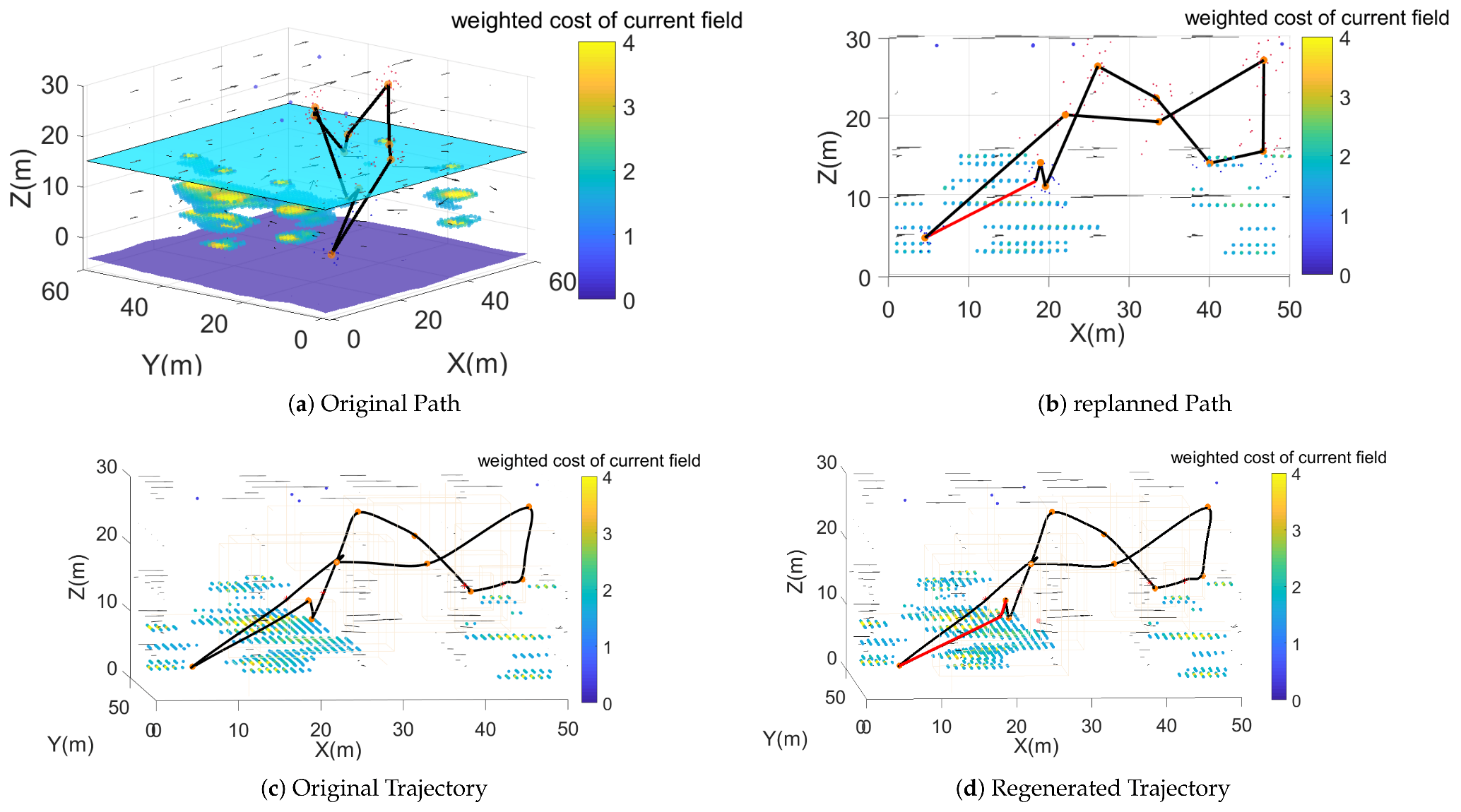
Figure 21.
The replanned path and trajectory in current fields. The weighted costs of recorded strong currents fields are illustrated. The original path and trajectory passed through or quite near to (distance < vehicle length) strong current fields, which would be unsafe and involves a high energy cost. The replanned path and trajectory avoided such areas. The weighted cost of avoiding the current was 770.2315, and to not avoid it was 810.1669 in this case.
Figure 22.
Outputs of 100 runs are scattered, and the average values are illustrated as lines. Generally speaking, heuristic performed better than a common TSP solver.
Figure 22.
Outputs of 100 runs are scattered, and the average values are illustrated as lines. Generally speaking, heuristic performed better than a common TSP solver.
Figure 23.
Outputs of 100 runs are scattered, and the average values are illustrated as lines. Generally speaking, with current fields, heuristic performed better than a common TSP solver. The total weighted cost changeed slightly with currents. The average velocity of current was 0.26 m/s underwater, and it was 0.97 m/s in the air.
Table 1.
Nomenclature.
| Variable | Description | Variable | Description |
|---|
| P | The whole path. | | is denoted as the set of target spots the while is coordinate of the target spot in path. |
| The sub path in P, each sub path contains 5–10 path segment, which denote the length of path the HAUV can detect when path re-planning. | | The path segment between and . |
| The length of . | | The overall weighted edge of path segment. |
| The overall weighted edge of surface/air/water/current fields. | | The velocity with which HAUV move from to . |
| The acceleration with which HAUV move from to . | | The maximum velocity with which HAUV move from to . |
| The maximum acceleration with which HAUV move from to . | | is the set of randomly appeared unknown obstacles, and is the set of all spots’ coordinate of the obstacle. |
| Coordinate of all the spots in the obstacle. | | The minimum circumscribed circle/sphere of . |
| The collision free circle/sphere out of , which is an extension of | | The shortest distance between the obstacle and . |
| The minimum distance between and . | | KD-tree constructed by terrain map. |
| KD-tree constructed by obstacles. | | The function of trajectory. |
| The control parameter of scapegoat tree. | | The spots set of terrain map. (The barriers.) |
| is denoted as map of informative spots while are the coordinates of those spots. | | The force HAUV need to overcome without current fields. |
| The force HAUV need to overcome with current fields. | | The velocity of currents. |
| wing area of the HAUV. | | Density of air/sea water. |
| Coefficient of lift/fraction in air/sea water. | | The length of HAUV. |
| The covariance of the informative spots group. | | The expectation of the informative spots group. |
| The size of terrain map in simulation. | | The control parameter of current fields checking. |
Table 2.
The parameters chosen for the ACO in this work.
Table 2.
The parameters chosen for the ACO in this work.
| |
|---|
| Number of ants | 75 |
| Volatilization of pheromone trail | 0.2 |
| Influence of pheromone | 1 |
| Influence of heuristic values | 4 |
| The constant Q | 10 |
| The max times of iterations | 100 |
| Heuristic function | 1/D; where D is the weighted distance between two spots. |
Table 3.
The distances of GLNS and ACO paths. On average, the paths of ACO were times the weighted lengths of those of GLNS.
Table 3.
The distances of GLNS and ACO paths. On average, the paths of ACO were times the weighted lengths of those of GLNS.
| | | |
|---|
| 5 | 25 | 209.48 | 390.795 |
| 10 | 205 | 564.75966 | 909.442 |
| 15 | 426 | 640.2459 | 1076.1183 |
| 20 | 421 | 197.42732 | 199.3851 |
| 25 | 525 | 769.062302 | 1373.5974 |
Table 4.
This table shows a comparison between the scapegoat tree and KD tree reconstruction replanning methods. refers to the size of the original terrain map; R refers to the radius in which expected points are located; refers to the number of points this obstacle contains; refers to the number of potential expected points; refers to the time cost of scapegoat; refers to the time cost of reconstruction .
| | | | | |
|---|
| 100*100 | 100 | 121 | 121 | 0.6950 | 0.6240 |
| 20*20 | 100 | 441 | 121 | 0.2030 | 0.2710 |
| 20*20 | 10 | 441 | 121 | 0.4490 | 0.2840 |
| 20*20 | 10 | 121 | 411 | 0.2070 | 0.1900 |
| 20*20 | 100 | 36 | 121 | 0.940 | 0.1080 |
Table 5.
The weighted distance costs of planned paths with and without current fields. There are small differences between the outputs of these two scenarios. A possible reason is the positive and negative influences of current fields offsetting each other.
Table 5.
The weighted distance costs of planned paths with and without current fields. There are small differences between the outputs of these two scenarios. A possible reason is the positive and negative influences of current fields offsetting each other.
| | | |
|---|
| 5 | 25 | 209.48 | 212.3 |
| 10 | 205 | 564.75966 | 541.3 |
| 15 | 426 | 640.2459 | 650.2432 |
| 20 | 421 | 197.42732 | 205.4523 |
| 25 | 525 | 769.062302 | 777.8012 |


