Abstract
For complex systems, it is not easy to obtain optimal designs for the hardware architecture and control configurations. Every design aspect influences the final performance, and often the interactions of the different components cannot be clearly determined in advance. In this work, a novel co-design optimization method was applied that allows the optimal placement and selection of actuators and sensors to be performed simultaneously with the determination of the control architecture and associated controller tuning parameters. This novel co-design method was applied to a state-space model of a downscaled active car suspension laboratory setup. This setup mimics a car driving over a specific road surface while active components in the suspension have to increase the driver’s comfort by counteracting unwanted vibrations. The result of this co-design optimization methodology is a Pareto front that graphically represents the trade-off between the maximum performance and the total implementation cost; the co-design results were validated with measurements of the physical active car suspension setup. The obtained controller tuning parameters are compared herein with existing controller tuning methods to demonstrate that the co-design method is able to determine optimal controller tuning parameters.
1. Introduction
Multi-domain engineering is becoming increasingly important in the development of modern products and machines. The design of such complex systems has therefore become a comprehensive design challenge. Conventionally, the different domains of system design are addressed sequentially and thus separately. First, a mechanical engineer makes decisions on the physical setup in accordance with properties regarding strength, inertia, weight, etc. In addition, a choice is made on the location of actuators and sensors and which parts of the system are correspondingly measured or controlled. Additionally, selection of the types of actuators and sensors is done. The mechanical engineer will try to make the correct choices of hardware components based on some assumptions regarding the performance to be achieved and the total implementation costs. After that, the control engineer designs a control configuration for the fixed hardware architecture. The application of different control architecture features can be considered, while corresponding controller tuning parameters must be determined. In contrast to the mechanical engineer, the control engineer uses different objectives, such as system stability, reference tracking properties, and disturbance rejection.
This sequential hardware architecture and control configuration design will cause problems when designing complex and interacting systems, resulting in sub-optimal system performance. First of all, in practice, the mechanical engineer and the control engineer almost completely ignore the tight interdependency between the hardware architecture and the control configuration on the overall performance. For example, choices made by the hardware engineer can already severely limit the design space of the control engineer. On the other hand, it is not always clear what the influence of specific design choices is on the final performance of the total system. Therefore, more and more attention is being paid to resource-efficient system design with a growing demand for systematic and comprehensive methods to obtain optimal co-designs of hardware architecture and control configurations [1].
This co-designing of hardware architecture and control configuration has only been applied to a limited extent. Examples of the co-designing of geometric properties and controller tuning parameters for a four-bar system (using a Genetic Algorithm), parallel robots (using a differential evolution), and machine tools (using a multilevel decomposition) can be found in [2,3,4], respectively. Similarly, co-designing of controller tuning through the use of a Linear Quadratic Regulator (LQR) method and the geometrical properties of a pendulum system, a satellite altitude control, and an angular motor controlling a mass position was detailed in [5,6,7], respectively. More recently, ref. [8] combined mechanical design properties and the PD controller tuning for an airborne wind energy system. Other controller tuning methods are also used in the co-designing of the controller tuning and mechanical design variables. For example, refs. [9,10] used the / method to obtain the controller tuning parameters. PID values can also be directly optimized, as shown in [11] for a DC motor. In [12], an example is shown in which the co-design of mechanical design variables and controller parameters was performed for a hybrid power train system used in a hydraulic excavator.
The co-design examples mentioned so far succeed in the simultaneous optimization of separate hardware parts and controller tuning for fixed and rather modest feedback loops. In contrast, the author of this work recently proposed an optimization methodology to perform a thorough co-design of the hardware architecture and control configuration [13]. The proposed methodology can perform a hardware architecture and control configuration co-design in which more parts can be optimized at the same time, while considering more extensive and also changing controller architectures. By doing so, a larger design space is explored to obtain a system-level optimum. The optimization methodology does not assume a fixed control architecture, but instead, a trade-off can be made between different control architecture features, which has not been considered in current literature before. Furthermore, the optimization methodology enables the inclusion of non-linear constraints and (conflicting) objectives. These objectives will always be related to the trade-off between implementation cost and system performance, represented in a Pareto front. This profound level of co-design has not been applied in the current literature.
Earlier work by the author suggested using a Genetic Algorithm (GA) [14] to optimize the proposed problem because it is one of the few algorithms that can satisfy the applicable non-linear constraints and intended objectives [13]. These objectives can be freely programmed according to, for instance, tracking error, vibrations, energy consumption, or settling time requirements. Additionally, non-linear (mixed-integer) constraints on, for example, maximum actuator output or hardware cost can be taken into account. A disadvantage in applying a Genetic Algorithm is that a relatively long calculation time is required. Genetic algorithms have previously been implemented for many applications, for instance, to determine the optimal controller tuning parameters using a Linear Quadratic Regulator (LQR) [15], control [16], or proportional integral (PI) control [17]. Another field of application of Genetic Algorithms is the motion profile optimization for repetitive machines [18].
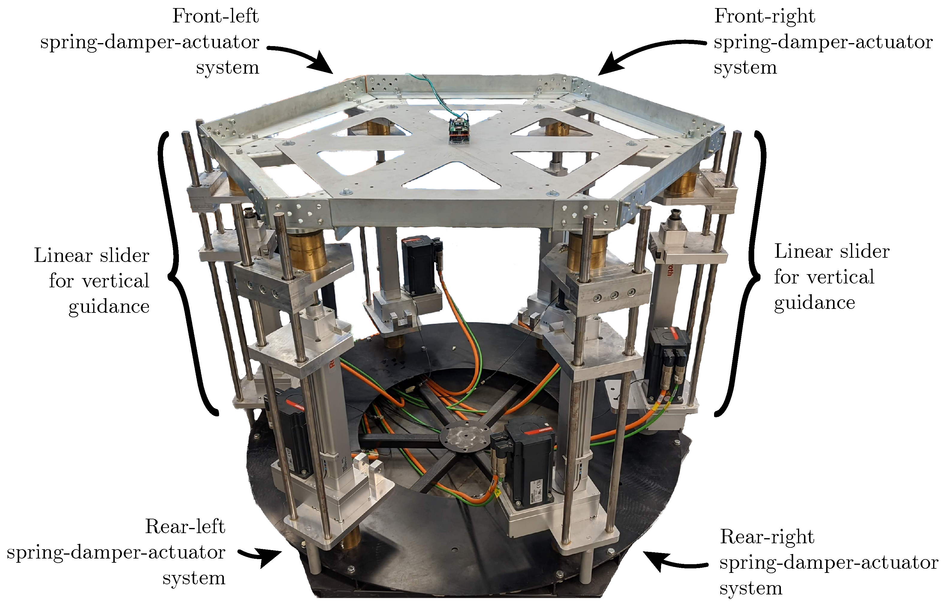
In this paper, the novel co-design methodology is applied to a state-space model of a downscaled active car suspension setup (see Figure 1). Over the past decades, active suspension control technologies became an extensive research topic; hence, these systems have a significant influence on the vehicle dynamics and the subjective driver comfort impression [19]. An example of previous work using a Genetic Algorithm (GA) to optimize feedback controller values via the Linear Quadratic Regulator (LQR) method for a quarter-car suspension can be found in [20]. Furthermore, refs. [16,21] used a Genetic Algorithm to optimize a robust controller for a vehicle suspension control. These optimizations were limited in the sense that only the controller tuning parameters were optimized. Additionally, mechanical design parameters and their influences on vehicle dynamics were optimized in [22,23]. More information on the theory and application of vehicle dynamics can be found in [24]. The laboratory setup that was used for this study mimicked the behavior of a car driving on a road surface while active suspension components ensure the driver’s comfort. The test setup allowed examining a wide variety of hardware architectures and control configurations. It is important to emphasize that the primary goal of this setup was not to improve the current state-of-the-art in active car suspension systems but rather to validate the presented model-based co-design methodology with measurements on a physical setup.

Figure 1.
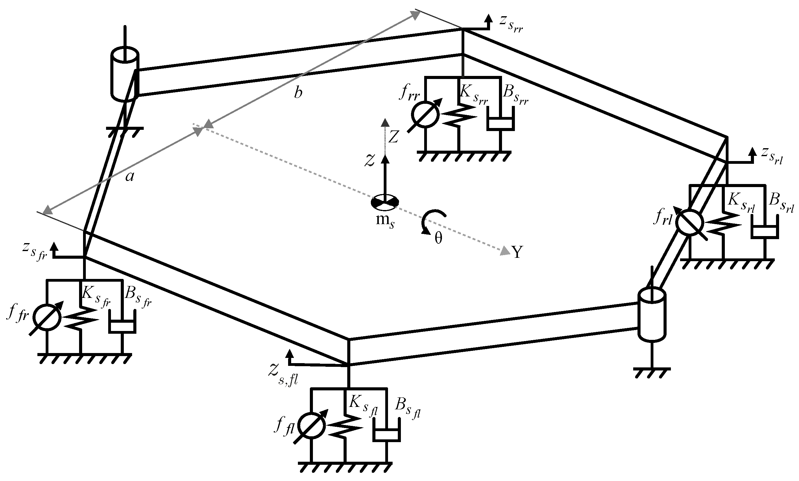
Picture of the physical full-car active suspension laboratory setup. The locations of the sliders and the spring-damper-actuator systems are indicated in accordance with the diagram in Figure 2. The linear slider systems for vertical guidance also had an actuator, but these were not connected to use the laboratory setup as in an active car suspension. The springs are not present in this picture, but were mounted to perform the mentioned tests.
The paper is organized as follows. Section 2 details the downscaled physical laboratory setup and the corresponding model description on which the co-design method was validated. Subsequently, Section 3 describes the application of the co-design methodology and its properties. The results of this model-based optimization and the validation measurements on the laboratory setup are presented in Section 4. Finally, conclusions are formulated in Section 5.
2. Active Car Suspension Setup
2.1. Setup Properties
A full-car active suspension laboratory setup was built to emulate the behavior of the widely available theoretical full-car suspension model [25,26,27,28]. The physical laboratory setup is shown in Figure 1, with the corresponding laboratory setup model diagram shown in Figure 2. The setup consisted of a central, hexagonal platform with mass supported in four places by a spring, a damper, and an actuator system in parallel. The spring-damper systems correspond to a classic car’s suspension, while the actuators represented an active component to counteract the unwanted vibrations of the central platform. The lower sides of the vertical rods could not translate but could rotate around their attachment points through ball couplings. The upper sides of the vertical rods were also attached to the central platform using ball couplings. Linear sliders were provided on the two opposite sides of the central platform, allowing the central platform to translate along the z-axis with a heave height z and rotate around the y-axis with an angular pitch rotation . This makes it possible to emulate a car driving on a straight road.

Figure 2.
Full-car active suspension laboratory setup diagram.
The key parameters to represent a passenger car suspension model are not the same for every car, but typical values can be found in previous work [19,23,25,27,29]. The laboratory setup has a scaling factor of 1:2 compared to typical mid-size passenger car dimensions. Therefore, the appropriate scaling laws must be applied for some fundamental parameters (see Table 1) [30]. Although the laboratory setup parameters do not perfectly match the downsized values of a typical passenger car, they are close enough so that the laboratory setup will exhibit similar dynamic characteristics to a typical mid-size passenger car.

Table 1.
Downscaling typical passenger car parameters to laboratory setup parameters with scaling factor 1:2.
2.2. State-Space Model Identification
The system has four inputs, namely, the four actuator forces , , , and . The subscripts , , , and represent the wheel location, being front-right, front-left, rear-right, and rear-left, respectively. These system inputs are used for both the application of the road profile disturbances , , , and (see Section 2.3) and the control effort signals , , , and eliminating unwanted central platform vibrations. The applied feedback control has no information on the road disturbance signals. The model inputs are as follows:
with . The model states are the horizontal position z, speed , acceleration , and angle of the central platform:
while the same system properties are used for the model output for the identification procedure:
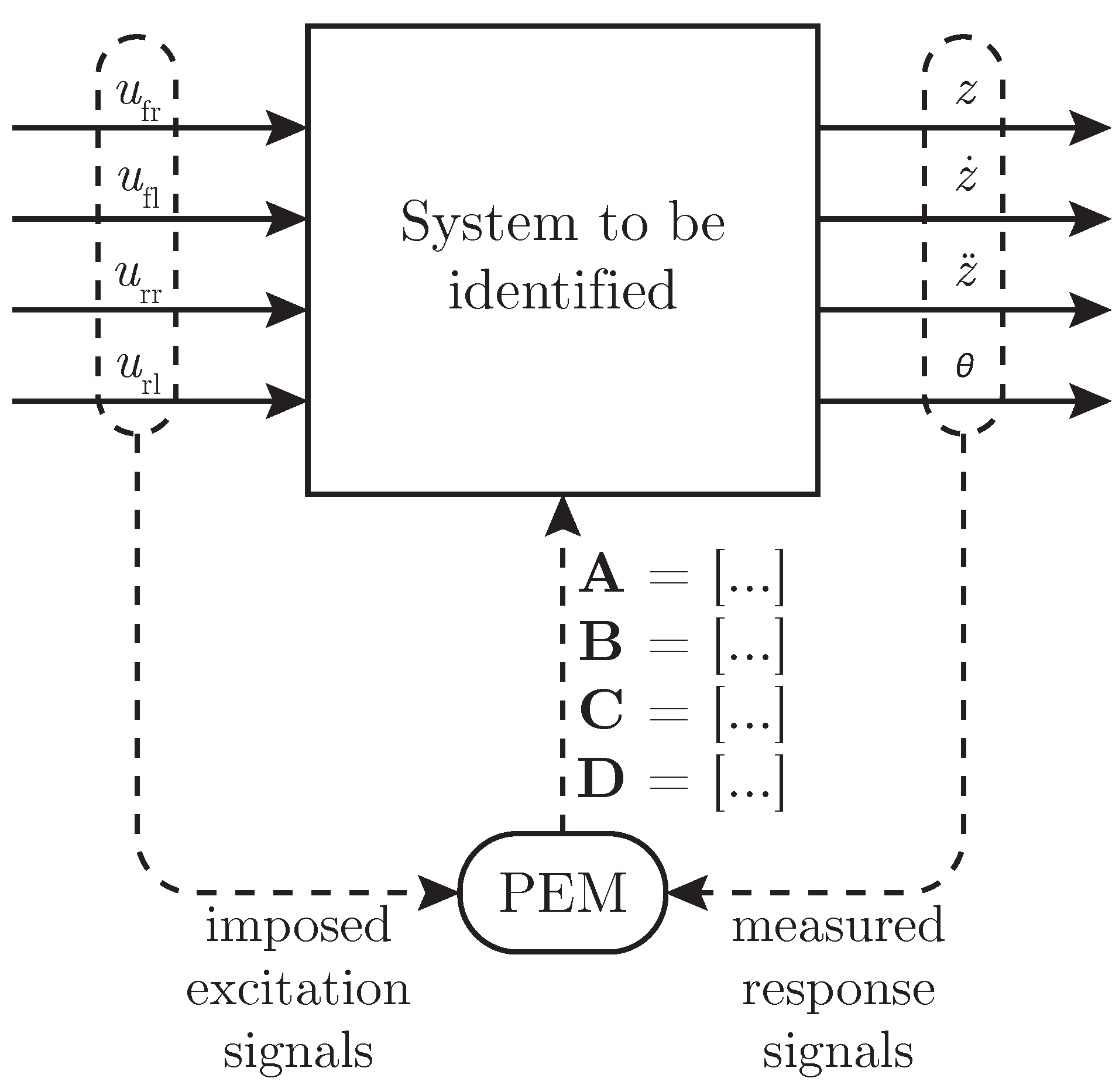
As a result, the dimensions of the state-space system matrices are defined as , , , and . For the model identification, a multisine excitation with sample frequency Hz containing sine frequencies from 0.01 Hz to 490 Hz [31] is imposed on the system inputs, while the system response is measured. From the measured input and output signals, the model matrices values are identified using the prediction error minimization (PEM) method [32]. This model identification procedure is graphically displayed in Figure 3.

Figure 3.
Graphical representation of the model identification procedure using a prediction error minimization (PEM) method to identify the system’s state-space matrix values based on the imposed excitation signals and measured response signals.
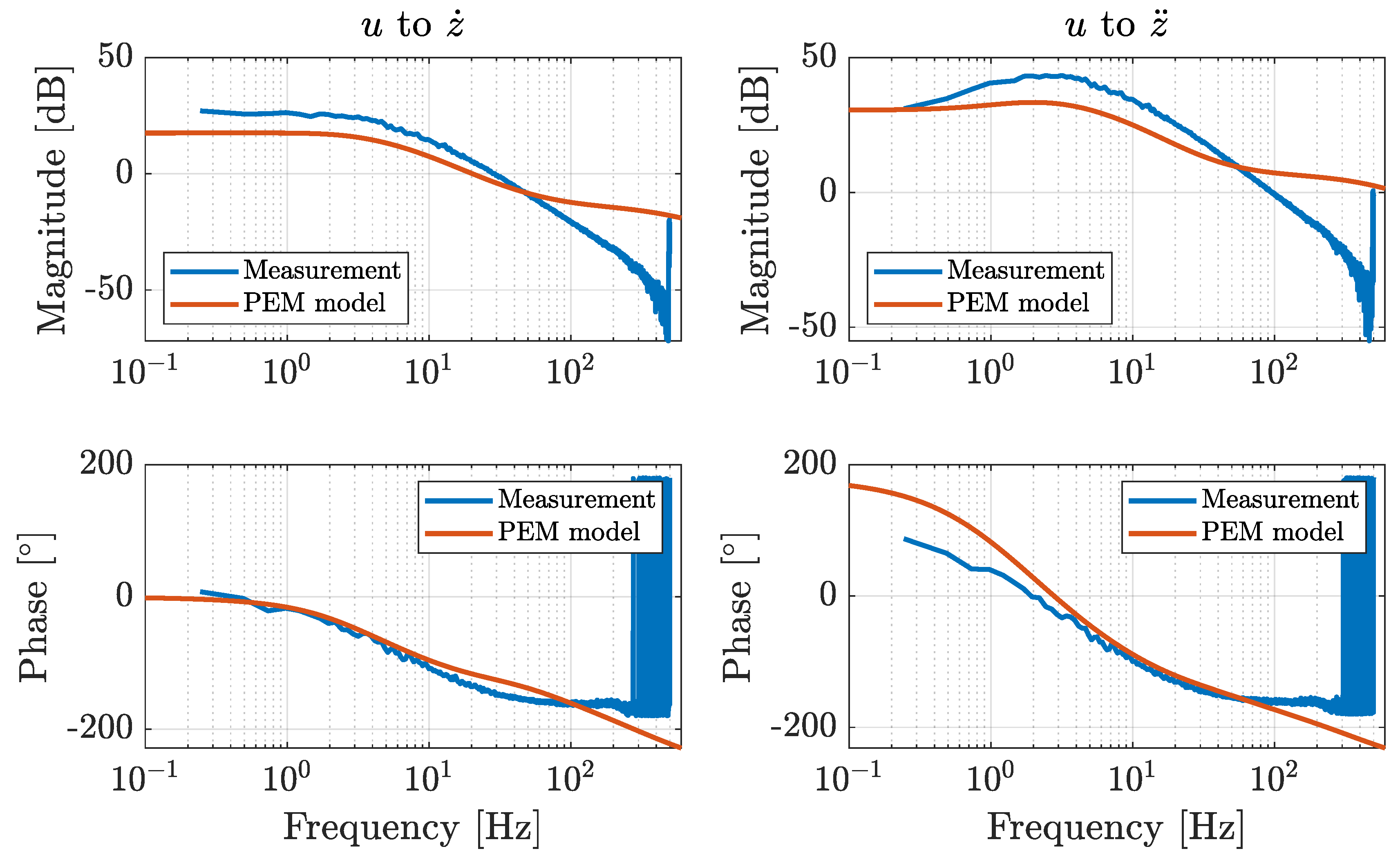
The resulting (rounded) matrix values are shown in Equations (4)–(7). Figure 4 depicts the Bode plot of the identification measurements using the multisine signal and the Bode plot of the identified PEM state-space model. It is important to emphasize that the model will not perfectly match the actual setup. For example, it is known in advance that the dampers have a non-linear character. This non-linear behavior (along with possibly other phenomena such as static friction) is not explicitly modeled in the identified Linear time-invariant (LTI) system.

Figure 4.
Comparison of the Bode plots of the identification measurements (blue) and the identified prediction error minimization (PEM) state-space system (red) from system inputs u to platform velocity (left) and system inputs u to platform acceleration (right).
2.3. Road Profile
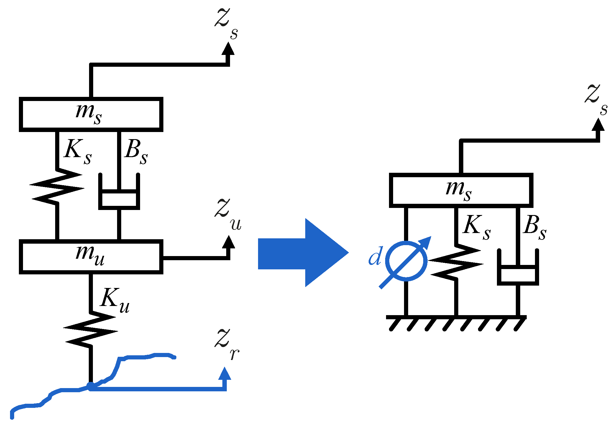
Road profile disturbance signals were applied to the actuators with the intention of the central platform experiencing the same forces as if it was driving over a real road surface. A random road profile formulation was based on the ISO 8608 norm, with a “roughness factor” indicating how smooth the road surface is. This factor ranges from 1 to 8 for smooth asphalt layers to very rough cobblestone roads [33,34]. The road profile is defined as a displacement disturbance, while the laboratory setup only allows force disturbance inputs. That is why the road displacement is converted to a force disturbance d for the active car suspension laboratory setup. This conversion is graphically represented in Figure 5.

Figure 5.
Graphical representation of the conversion from a road displacement from a traditional quarter car model to a force disturbance d for the quarter-car suspension laboratory setup.
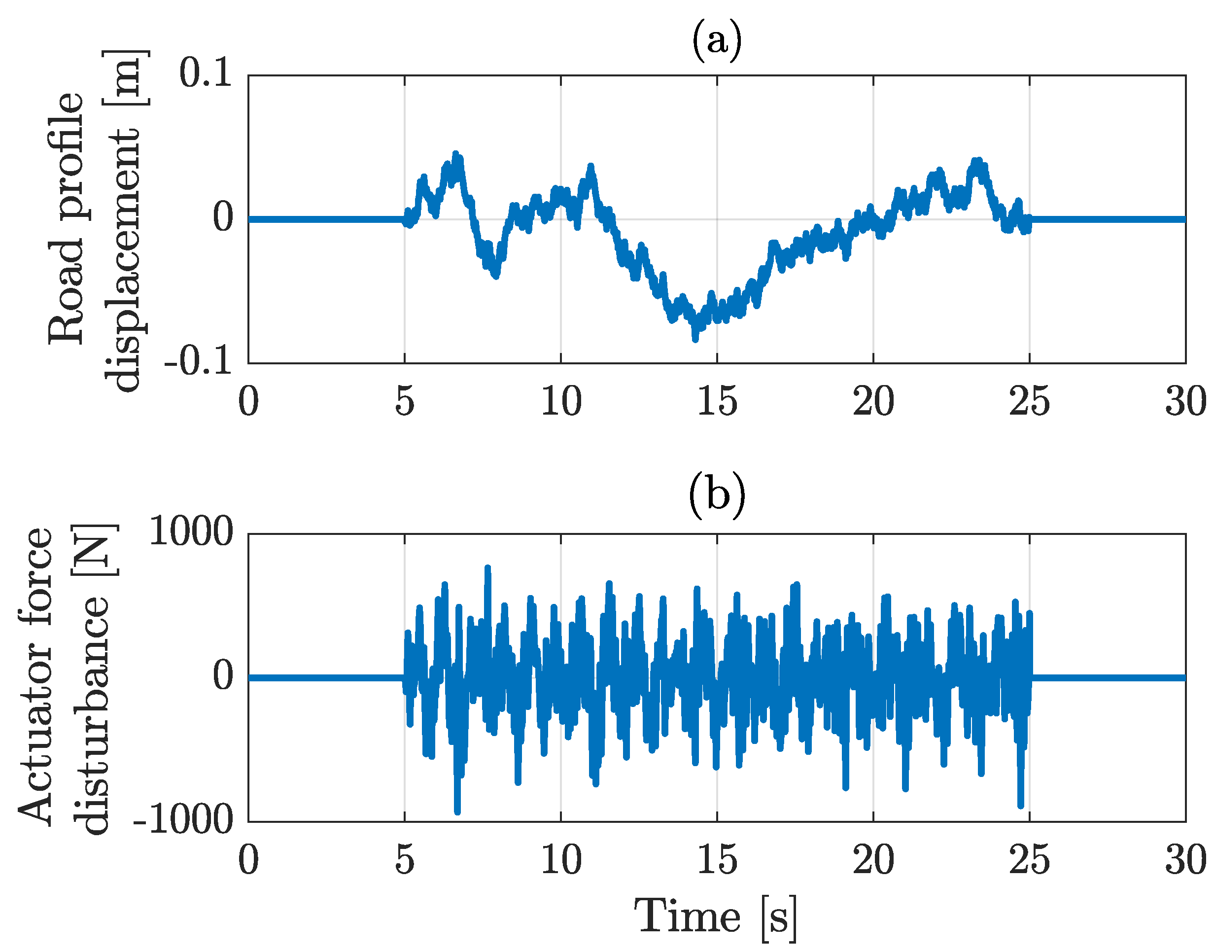
Figure 6a shows an ISO 8606 road profile for a car traveling at 72 km/h for 20 s on a road profile of 400 m with a roughness factor 5. Figure 6b shows this displacement profile converted to an equivalent force profile, applicable to the laboratory setup. Based on a speed of 72 km/h and a distance between the front and rear wheel axles of 1 m, there will be a time delay of 0.05 s between the applied front and rear wheel force disturbances.

Figure 6.
(a) ISO 8608 road displacement profile with roughness factor 5. (b) Corresponding actuator force disturbance.
3. Hardware and Control Co-Design
3.1. Objective Function
The objective of the active car suspension setup is to achieve the greatest comfort for the driver. According to the ISO 2631 norm, the driver’s comfort is quantified as the perceived acceleration levels in the three principal axes [35]. The laboratory setup only allows translation along the vertical z-axis. That is why in this case, the control objective is to minimize the z-axis accelerations, maximizing the driver’s comfort. A fitness value (FV) quantifies the performance according to the ISO 2631 norm by taking the rms of the acceleration along the z-axis:
with N the total number of samples, being s/0.001 s = 30,000.
3.2. Design Parameters
The design parameters for this co-design optimization problem consist of two actuator selection integers, two sensor selection binaries, two control architecture binaries, and 12 controller tuning parameters.
The actuator selection integers and define which types of actuators are applied to the front wheels f and the rear wheels r, respectively. Table 2 provides an overview of the different actuator types, with each actuator type corresponding to an associated cost and maximum actuator output. The component cost was chosen arbitrarily and was different for each application. Therefore, this cost is not expressed in a currency but in percentage terms relative to the most expensive setup in which all possible parts were present.

Table 2.
Possible actuator selection integer values with corresponding cost and maximum actuator output.
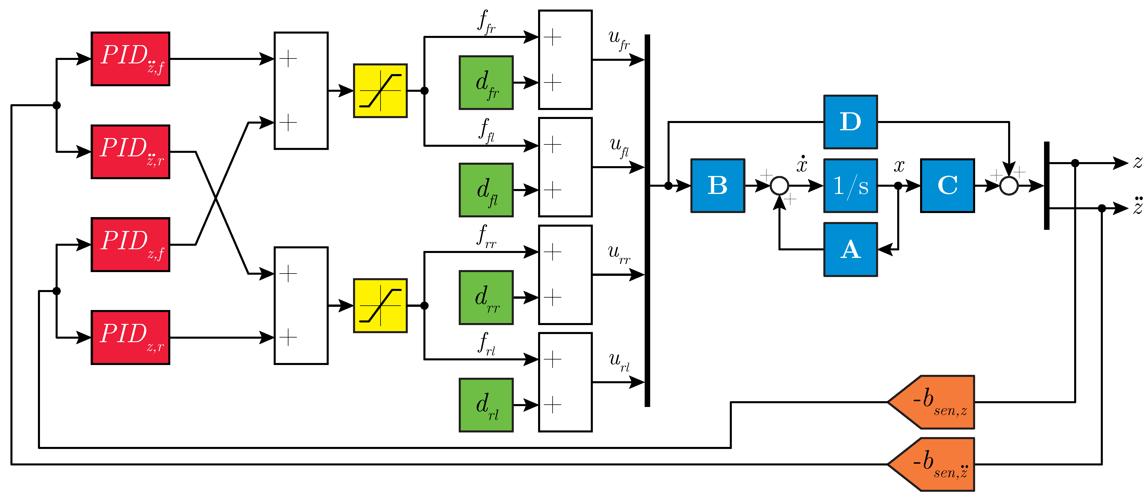
The design space for the feedback control architecture is shown in Figure 7. This design-space shows the attainable form of the feedback control when all capabilities regarding the control configuration optimization are active. The second and fourth row of the and matrices of the identified model are omitted for the co-design optimization procedure so that the model has the platform position z and acceleration as outputs. PID controllers can be applied separately to the front and rear wheels for both the displacement and acceleration feedback control. The sensor selection binaries and define the presence or absence of a sensor on the central platform heave position z and acceleration , respectively. The cost for a displacement feedback sensor and an acceleration feedback sensor is and , respectively. The control architecture binaries and define the presence or absence of the PID controllers for the displacement and acceleration feedback control, respectively. Both control loops have a cost of . The PID controller values , , and are also design parameters, with the subscript referring to the corresponding controller. For example, is the value of the acceleration feedback PID controller connected to the rear actuators.

Figure 7.
Design space for the feedback control architecture with the active car suspension model in blue, road profile force disturbance signals in green, actuator output saturation in yellow, PID controllers in red, and sensor feedback in orange.
3.3. Constraints
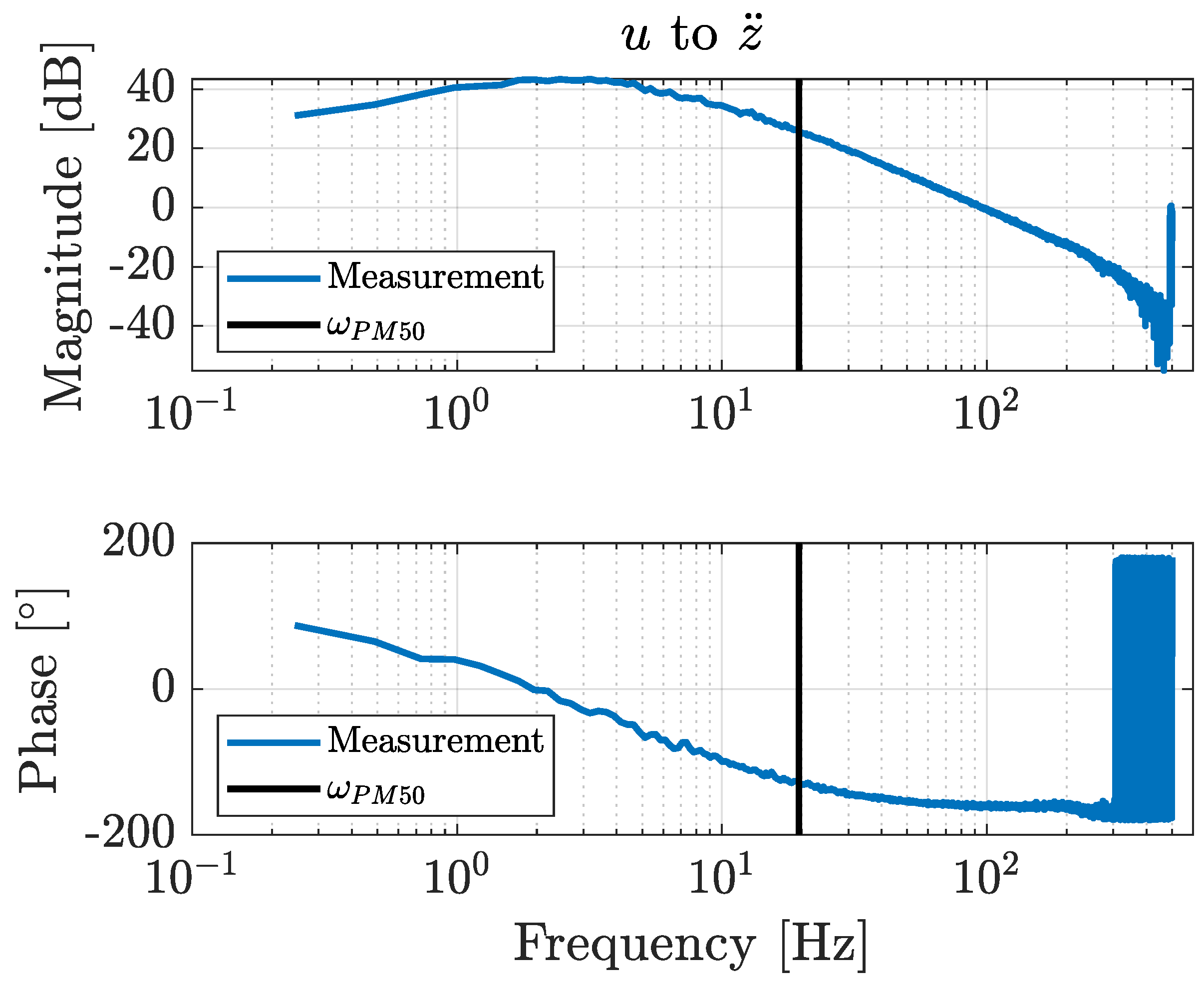
The number of possible actuator types determines the upper and lower bounds for the actuator selection integers, see Table 3. For the binary design parameters, the bounds are equal to zero and one. For the PID values, the most relaxed boundaries are determined based on system stability margins. For example, for determining the constraint on the upper bound of the acceleration feedback values and , a phase margin of is suggested to obtain a sufficiently robust control [36]. The Bode plot of the system input u to the platform acceleration identification measurements is shown in Figure 8. To obtain this phase margin of 50°, a zero crossing of the magnitude plot must occur at a phase angle shift of . The phase plot shows that a phase angle shift of −130° occurs at (illustrated with a black vertical line in Figure 8). The gain at phase is 25.96 dB. Thus, the corresponding gain factor is .

Table 3.
Design parameters with their corresponding lower bound (LB) and upper bound (UB) constraints.

Figure 8.
Bode plot of the identification measurements (blue) from system inputs u to platform acceleration . A vertical black line indicates frequency at which the phase plot attained –.
Table 3 provides an overview of the design parameters with corresponding lower bound (LB) and upper bound (UB) constraints. Next to the design parameter bounds, a maximum implementation cost can be implemented as a nonlinear constraint in which the optimization algorithm ensures that the sum of the different components does not exceed this maximum implementation cost. By subsequently performing this optimization for several different maximum implementation costs, the progression of the maximum achievable performance relative to the total implementation cost can be determined.
3.4. Genetic Algorithm Application
A Genetic Algorithm (GA) was deployed to optimize the 18 design parameters based on the non-linear objective function and according to the mixed-integer and non-linear constraints mentioned above. For this active car suspension application, the optimization was performed repeatedly with a changing constraint on the maximum cost varying from to in 14 equal steps. By allowing a higher maximum implementation cost in successive optimizations, more expensive and higher performing parts could be used. In this way, the different points of the Pareto front were determined. Table 4 depicts some of the key settings for the Genetic Algorithm.

Table 4.
Genetic Algorithm settings.
Increasing the population size enables the Genetic Algorithm to search more points in one generation. However, the larger the population size, the longer the genetic algorithm takes to compute each generation. A population size of 300–500 individuals is suggested for the type of co-design optimization problems described in this paper. Successive generations are calculated iteratively using three “reproduction functions”: “elite selection”, “crossover”, and “mutation”. “Elite count” indicates how many individuals go directly and unchanged to the next generation through elite selection. This value is usually around 10–20 for this type of optimization problem [37]. The rest of the GA children are determined via crossover and mutation. A crossover child is formed by randomly combining variables from two parent individuals. A mutation child is created by randomly making small changes in the variables of a parent individual. The “crossover fraction” value specifies the fraction of the remaining children determined via crossover (and not via mutation). For optimization problems with a discontinuous objective function, it is recommended to set the crossover fraction low [38]. In this way, a relatively large number of mutations occur when determining the children, resulting in a broad search space for subsequent generations, preventing the optimization algorithm from prematurely ending up in a local minimum. An appropriate “crossover fraction” value is 0.4 for co-design optimization problems described in this paper. Refer to [39] for more in-depth information on the technical operation of a Genetic Algorithm. The optimization took approximately 8 hours and 18 minutes on an Intel® Xeon® CPU @ 3.10 GHz with 64 GB of RAM.
4. Results and Measurements
4.1. Model-Based Pareto Optimizations
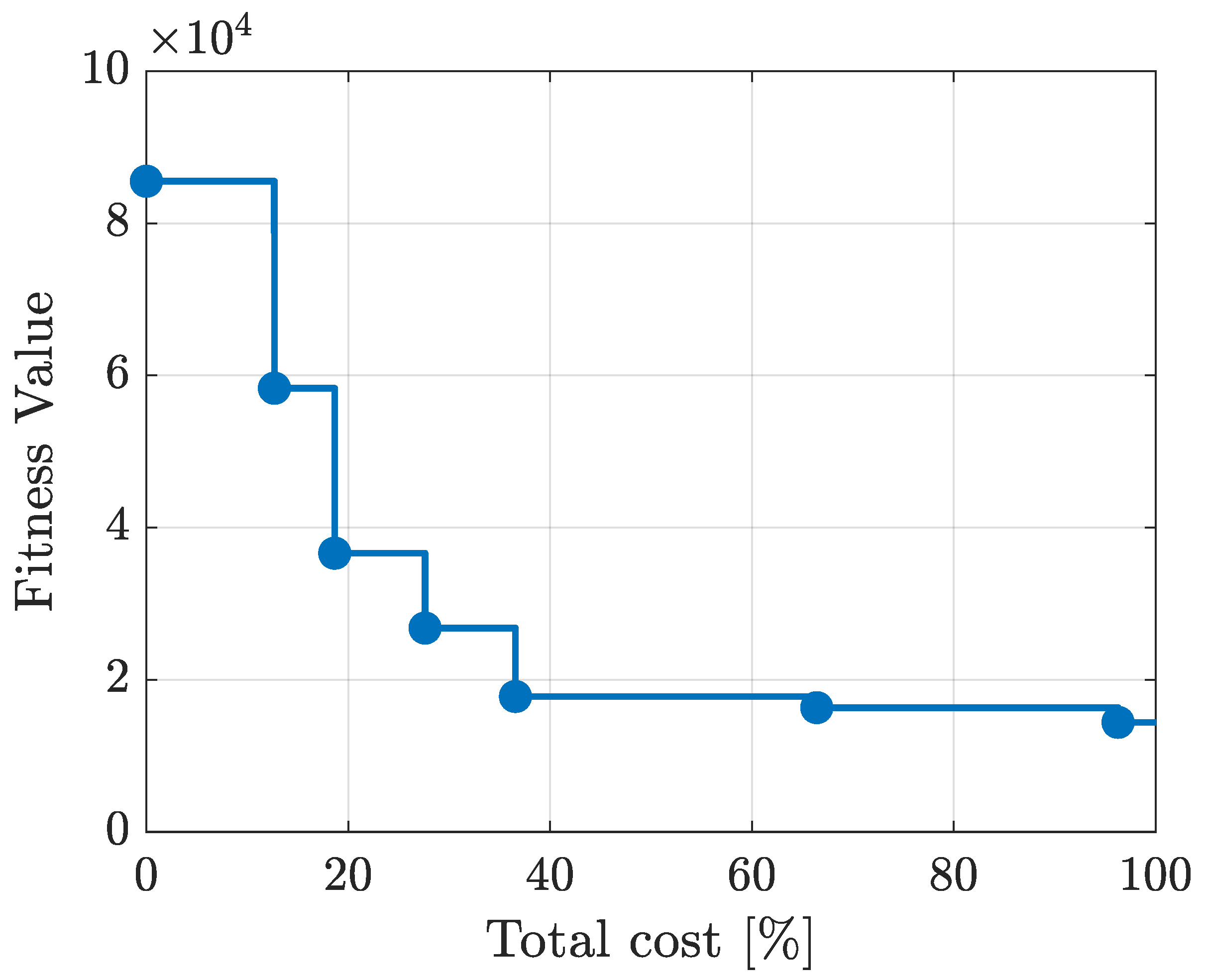
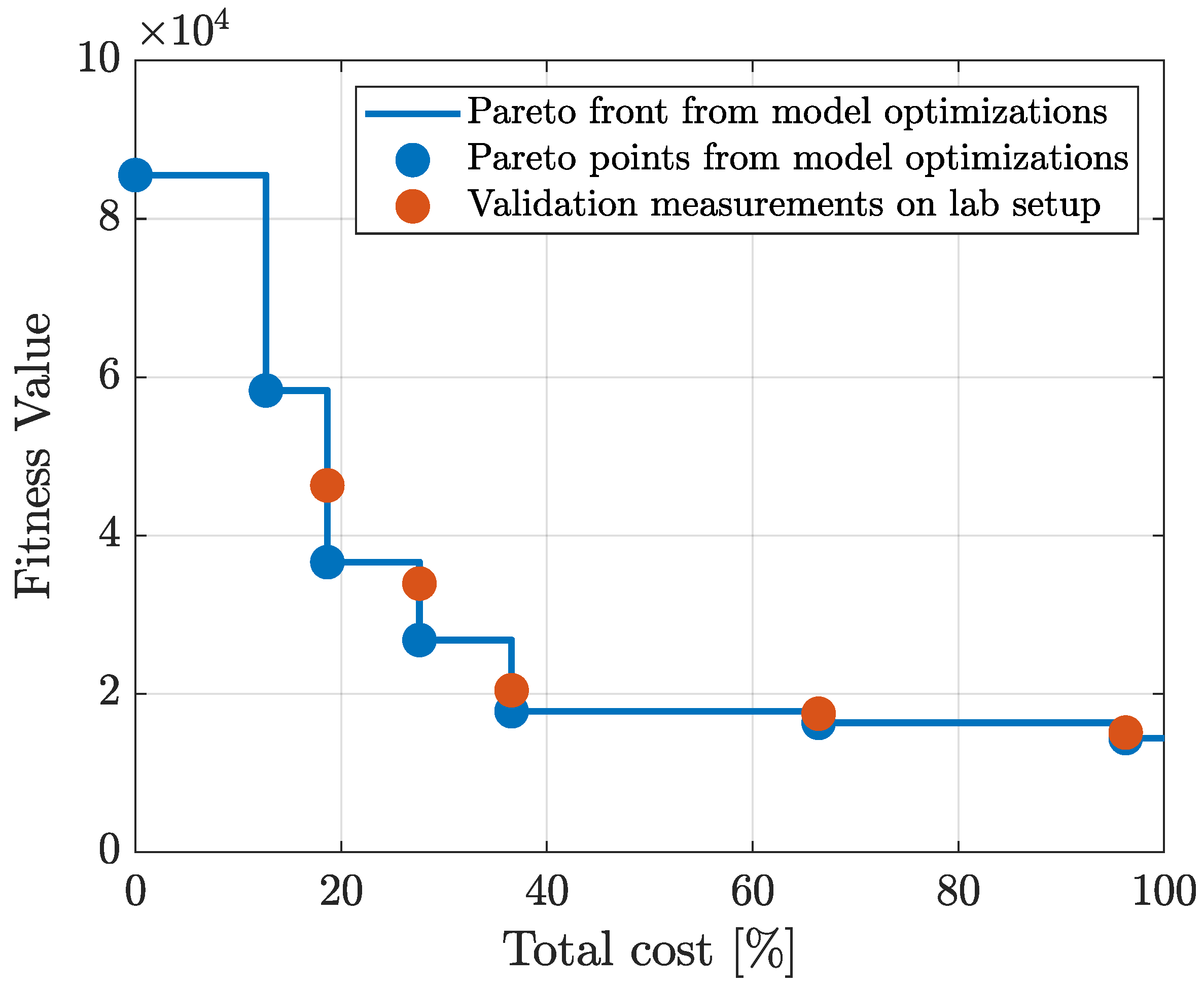
Table 5 shows the results for every Pareto point optimization. As more implementation costs are allowed, actuators with higher torque outputs can be applied, resulting in better fitness values, and thus, better system performances. Each point contains an optimized situation depending on the implementation cost. It will be up to the design engineer to make a final decision on which Pareto point is most appropriate for the specific application. None of the Pareto-optimized points contain a position feedback control. Thus, these results show that applying a position feedback control gives no added value to the intended objective. This is also why the last Pareto point does not have a cost of . The resulting Pareto front is shown in blue in Figure 9 and provides a valuable understanding of the trade-off between the performance and the implementation cost.

Table 5.
Model-based Pareto front optimization results (rounded).

Figure 9.
Pareto front representing the active car suspension model optimization results, showing the maximum achievable performance related to the implementation cost.
4.2. Validation Measurements
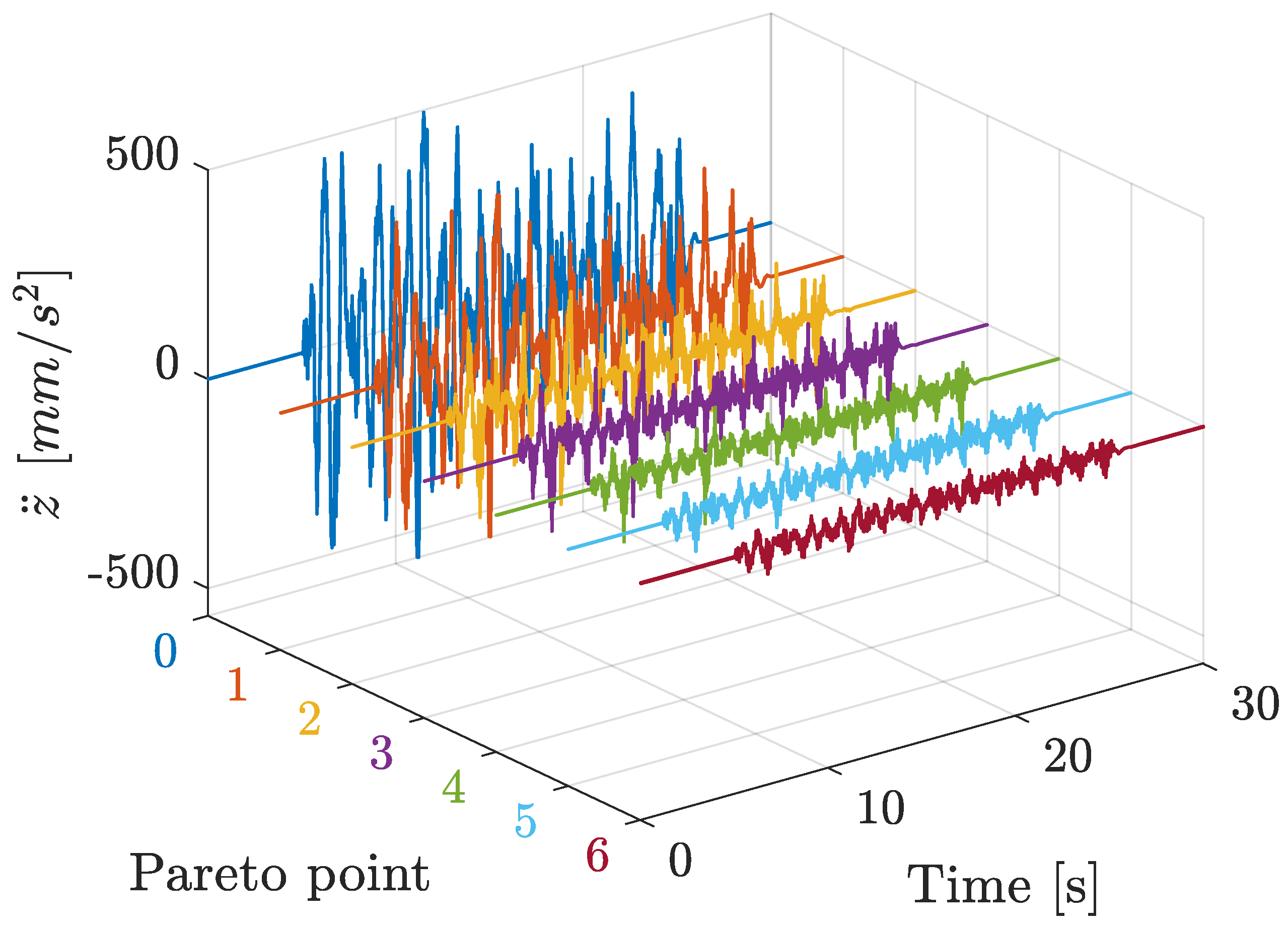
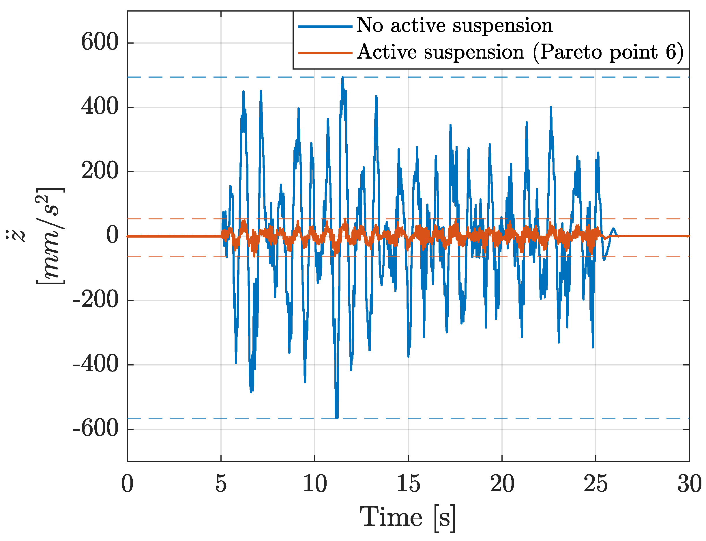
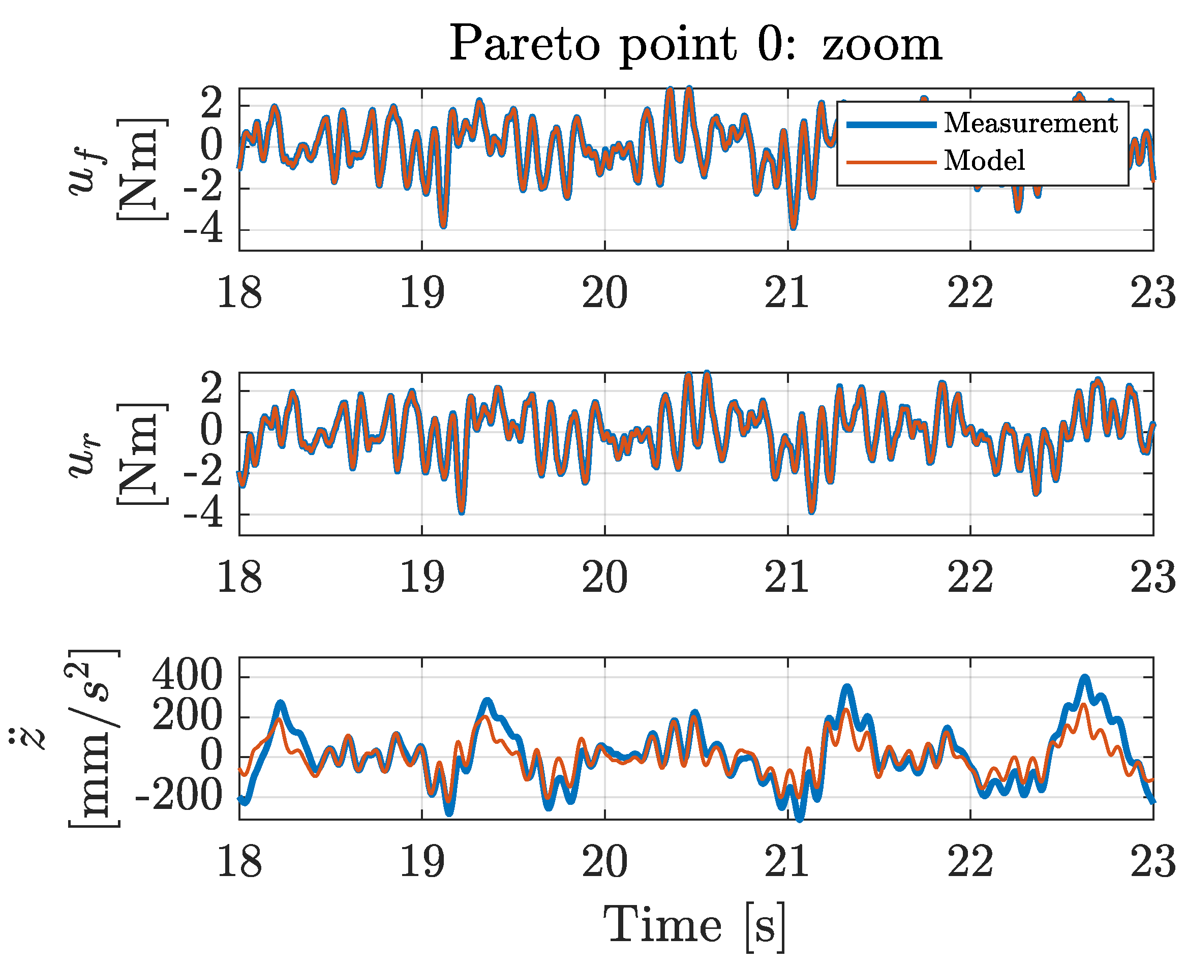
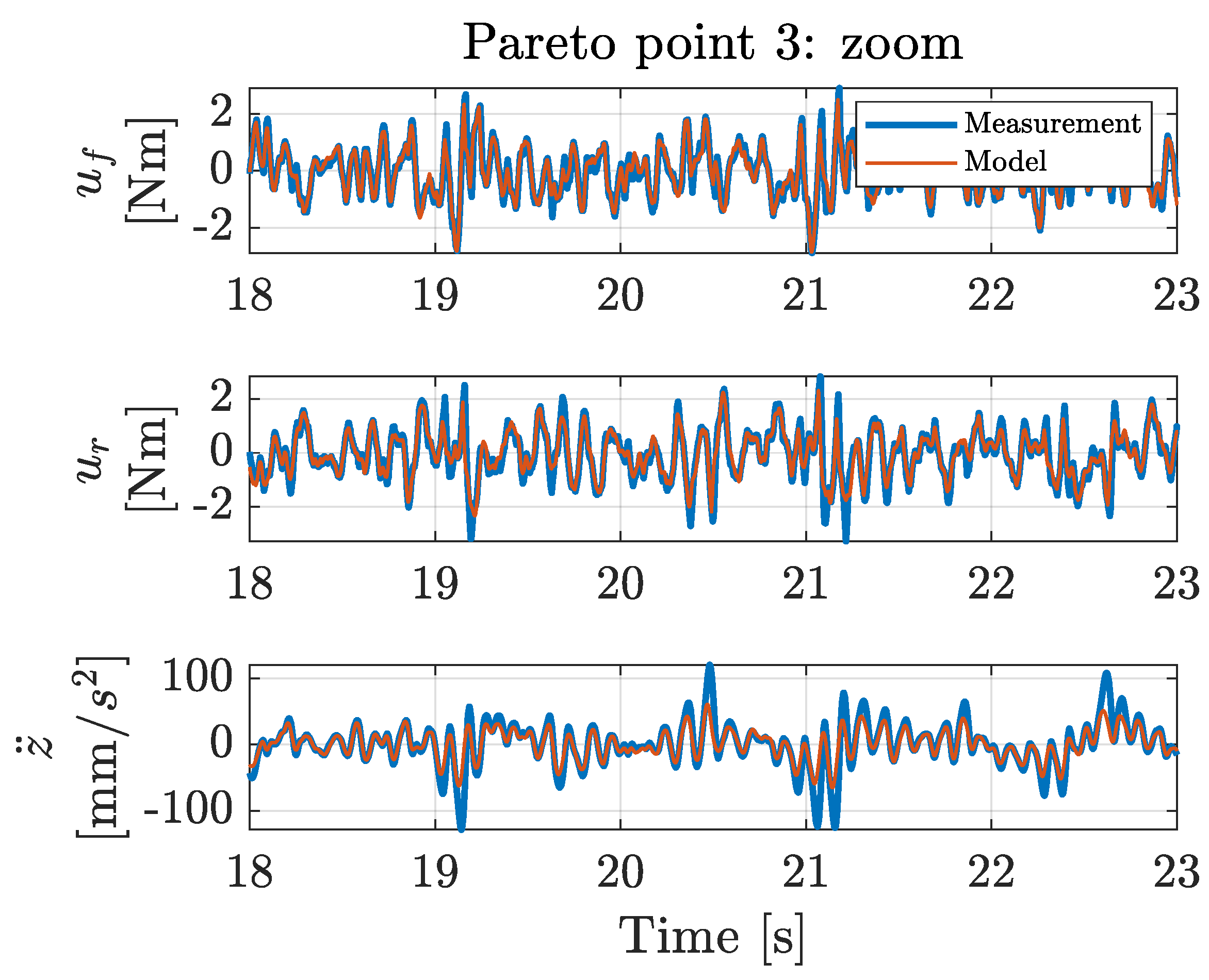
The results of the model-based Pareto optimizations were validated with measurements on the physical laboratory setup. For each hardware and control combination of Table 5, the system response to the same road disturbance signals was measured. Appendix A details the differences between the model-based calculated responses and the actual measured responses for each Pareto point, see Figure A1, Figure A2, Figure A3, Figure A4, Figure A5, Figure A6, Figure A7, Figure A8, Figure A9 Figure A10, Figure A11, Figure A12, Figure A13, Figure A14 and Table A1, Table A2, Table A3, Table A4, Table A5, Table A6, Table A7. Figure 10 depicts the platform acceleration measurements for every Pareto-optimized point configuration. The progression of the graphs clearly shows that the measured accelerations decrease as a higher maximum implementation cost is allowed. Figure 11 depicts the difference in platform accelerations measurements between no active actuation and the optimized active actuation from Pareto point 6. The figure shows that the largest acceleration spike decreased from −566 to −63 mm/s, which is a reduction of . This means that a significant increase in driver’s comfort can be achieved using the optimized active car suspension, which is also represented in the corresponding fitness values.

Figure 10.
Measured platform acceleration for every Pareto-optimized point configuration.

Figure 11.
Comparison of the measured platform acceleration for no active actuation (blue) and with optimized active actuation (red) from Pareto point 6 for the same road disturbance signals.
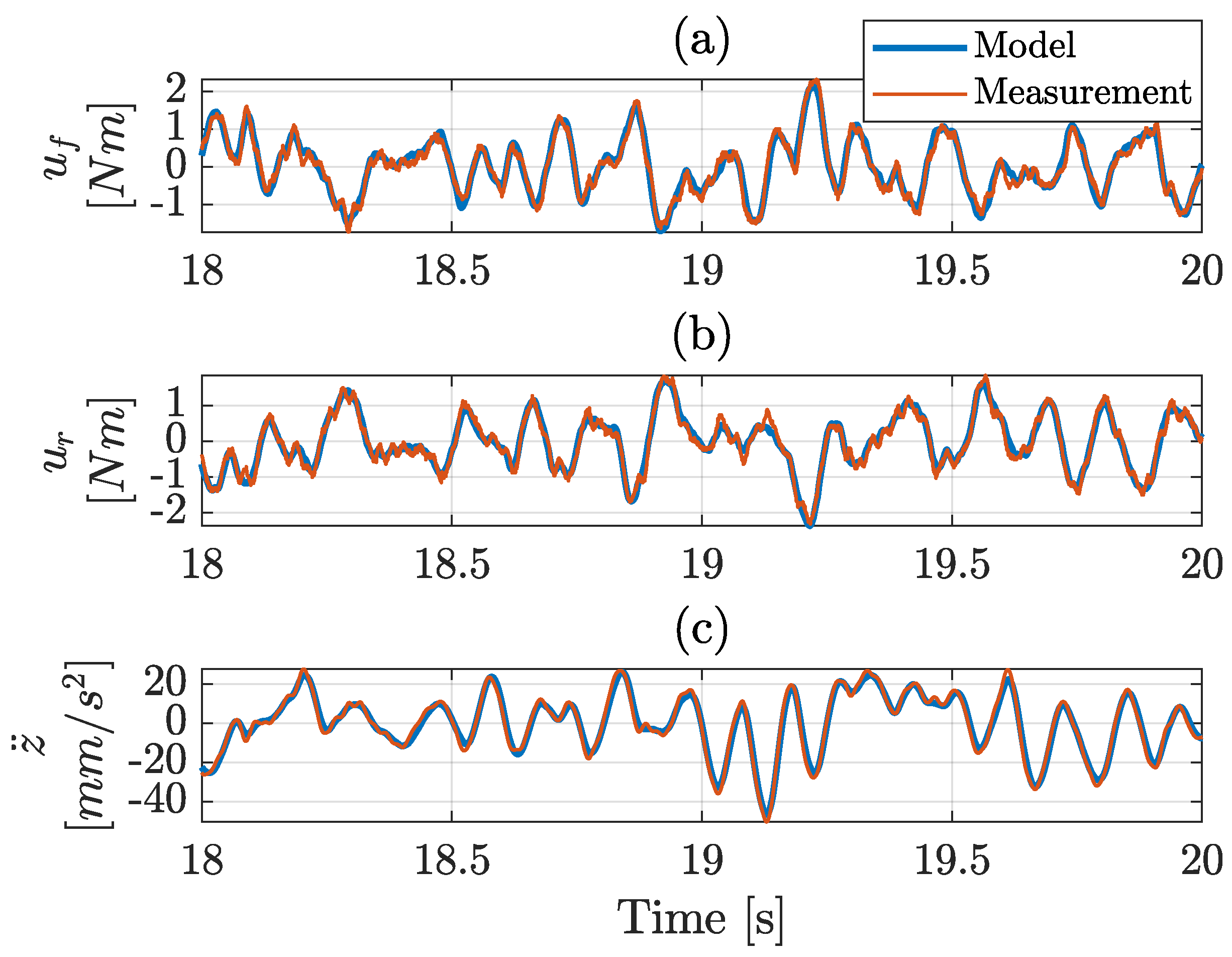
Figure 12 shows a comparison of the calculated and measured front and rear wheel actuator outputs and and platform acceleration signals for a part of the time-domain response for Pareto point 6, demonstrating that the calculated and measured responses match well. Table 6 shows the fitness values for the validation measurements. These validation measurement results are depicted together with the model-based Pareto optimization results in Figure 13. The calculated and measured fitness values show better agreement as more co-design features are allowed and the implementation cost rises. Although the individual measured fitness values for configurations with smaller implementation costs do not match the model-based calculated fitness values, the overall trend is similar to that of the calculated fitness values. Therefore, conclusions on the hardware and control co-design based on the model-based optimization values will still be valid on the physical setup. The differences mentioned above can be attributed to modeling errors (e.g., friction or non-linear system behavior) and inherent measurement noise levels in the actual setup rather than limitations of the optimization algorithm.

Figure 12.
Comparison of the calculated (blue) and measured (red) time-domain responses for the front wheel actuator output (a), rear wheel actuator output (b), and platform acceleration (c) for the validation measurement of Pareto point 6. The actuator outputs consist of the road disturbance signals and the control effort signals .

Table 6.
Fitness values for the model-based optimization results and the validation measurements.

Figure 13.
Comparison of the Pareto front results (blue) from the model-based co-design optimization methodology and the Pareto point validation measurements on the physical lab setup (red).
4.3. Comparison to Existing Controller Tuning Methods
The optimized controller values are compared here to existing controller tuning methods to validate the optimized acceleration controller tuning parameters as part of the control configuration optimization. First, the obtained controller tuning is compared to an LQR feedback design. In an LQR control design, relative weights are given to the state and input variables by adjusting the diagonal matrix Q and R values, respectively. Based on these values, a cost function minimization routine determines the values of the feedback matrices [15]. Thus, the LQR controller design comes down to adjusting the weights of the Q and R matrices according to the desired system behavior. However, for this application, a typical starting value of 1, applying the Bryson method [40], and manual adjustments of the Q and R diagonal matrices did not lead to a feasible solution. Thus, it was found that applying an LQR feedback control loop always leads to an unstable system, which is not the case with the controllers from the presented co-design methodology.
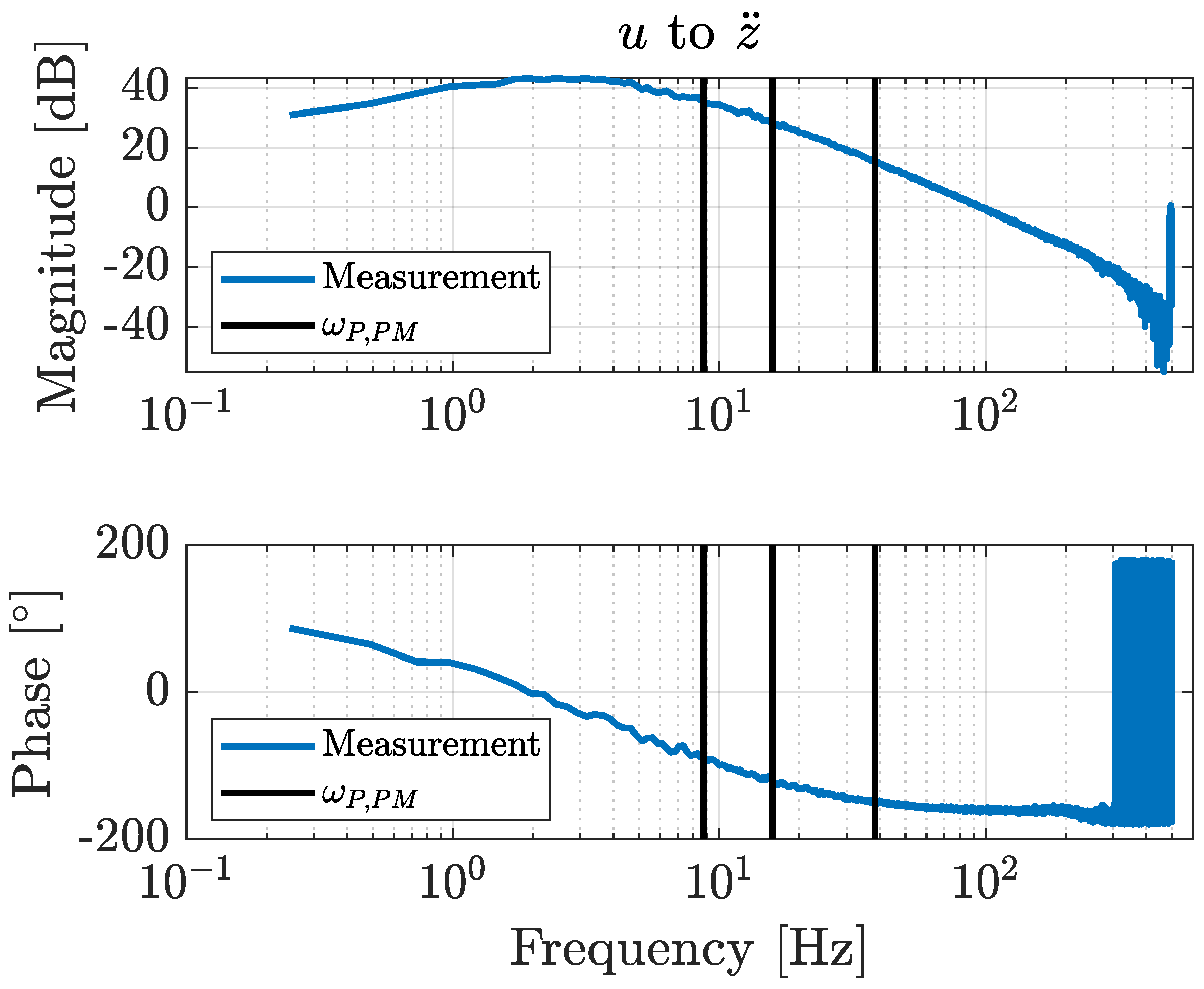
Furthermore, an existing controller tuning method was applied in which the P and PI controller values were determined based on the intended phase margins of the measured Bode plots [41]. This measured model is further denoted as G. The controller tuning method was applied to obtain P acceleration controllers with intended phase margins equal to 30, 60, and 90. Figure 14 shows the Bode plot of the identification measurements for G in which the frequencies , , and for phase margins of 30, 60, and 90, shown with black vertical lines. The corresponding , , and values are obtained by compensating for the differences in the magnitude ratio at , , and , respectively. Thereafter, each P controller was tested on the physical laboratory setup with different actuator types for a comparison with the obtained Pareto points from the co-design optimization methodology. Table 7 shows the results for the existing P controller tuning method and the corresponding validation measurements.

Figure 14.
Bode plot of the identification measurements from system inputs u to platform acceleration with frequencies , , and shown in vertical black lines to define the corresponding P controller values.

Table 7.
Existing P controller tuning and validation measurement results for different phase margins. The fitness values for unstable system configurations are denoted by “/”.
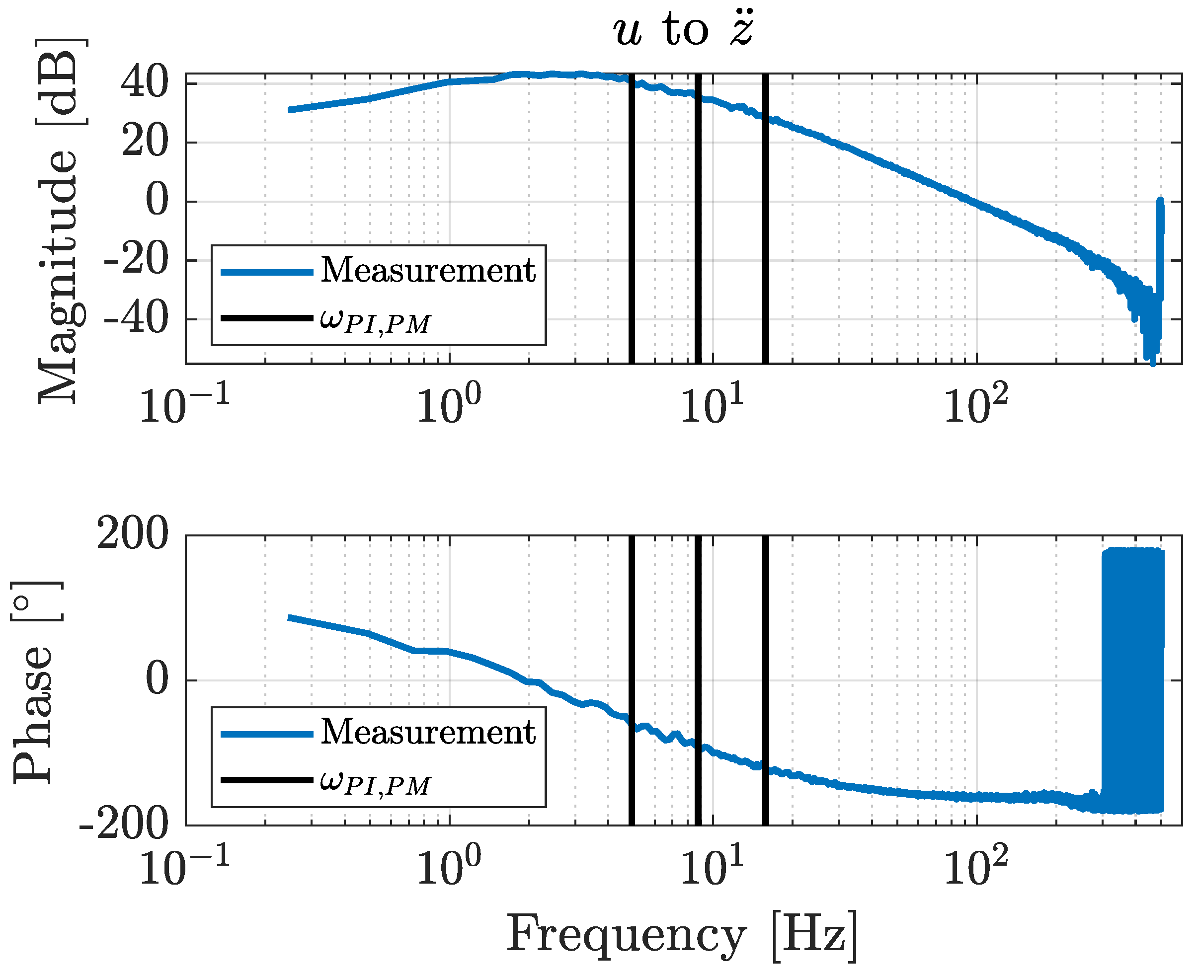
The same approach was used to obtain PI acceleration controllers with phase margins of 30, 60, and 90 at corresponding frequencies , , and . A PI controller consists of a gain, a pole at the origin, and a zero [42]. The pole will cause a phase delay of −90 at the frequency at which the magnitude plot crosses 0 dB. A zero causes a phase angle shift of +90 for infinitely high frequencies, but it is more realistic to design the controller requiring a phase shift of +60 at frequency . With this knowledge, the frequency can be determined as:
Figure 15 shows the Bode plot of the identification measurements in which the frequencies , , and for phase margins of 30, 60, and 90 are shown with black vertical lines.

Figure 15.
Bode plot of the identification measurements from system inputs u to platform acceleration with frequencies , , and shown in vertical black lines to define the corresponding PI controller values.
Once frequency is defined, can be specified as:
from which the value of is found.
Finally, the value is determined so that the combined magnitude plot of the system and the PI controller intersects 0 dB at frequency . The obtained PI acceleration controllers were also tested on the physical laboratory setup with different actuator types. Table 8 shows the results for the existing PI controller tuning method and the corresponding validation measurements.

Table 8.
Existing proportional integral (PI) controller tuning and validation measurement results for different phase margins.
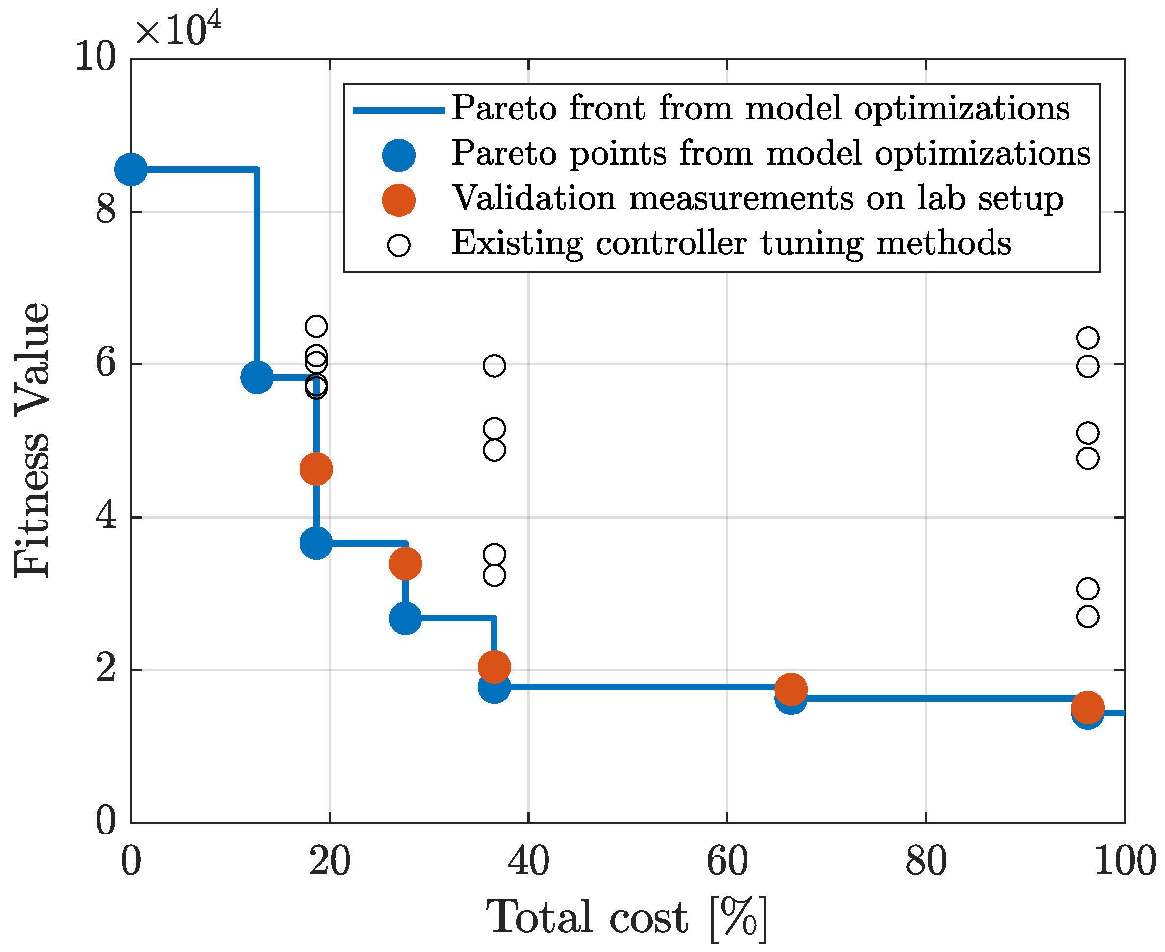
The measured performances of these P and PI controller tuning methods are depicted as black circles in Figure 16. As shown in this figure, no classical controller tuning method achieved the performance obtained with the optimized values determined by the co-design methodology proposed in this paper.

Figure 16.
Comparison of the Pareto front results (blue) from the model-based co-design optimization methodology, Pareto point validation measurements of the physical laboratory setup (red), and measurements of existing controller tuning methods (black).
5. Conclusions
In this work, a novel co-design optimization methodology was applied to an active car suspension laboratory setup. Initially, the setup dynamics were identified by applying a prediction error minimization method to obtain a state-space system representation. Actuator force disturbance signals were determined to mimic a situation in which a car is driving over an actual road profile. The active components in the car suspension were used to reduce the central platform vibrations so that the driver’s comfort was increased.
With the proposed co-design methodology, the optimal types and locations of actuators and sensors were determined simultaneously with the optimal control architecture and controller tuning parameters, exhibiting a profound level of co-design unprecedented in the current literature. This novel co-design methodology uses a Genetic Algorithm implementation, for which the results are presented in a Pareto front that graphically shows the interplay between the maximum achievable performance and the implementation cost. These results can be of great value to a design engineer in understanding how the maximum achievable performance varies as a function of the implementation cost.
The system configurations of the resulting Pareto points were validated with a physical laboratory setup. These validation measurements show that the obtained model-based trend in the Pareto front can also be observed in the corresponding measurements. The differences in the performances between the calculated and the measured situations can be attributed to the inherent measurement noise levels and modeling inaccuracies (e.g., friction or non-linear system behavior) rather than to errors in the co-design optimization methodology. Additionally, existing controller tuning methods were applied to the physical setup, and no existing method achieved the performance obtained with the proposed co-design methodology. This demonstrates that the presented co-design methodology is capable of determining the optimal controller tuning parameters.
Author Contributions
Conceptualization, M.H., S.D., K.S. and C.-M.I.; methodology, M.H., S.D., K.S. and C.-M.I.; software, M.H.; validation, M.H.; data curation, M.H.; writing—original draft preparation, M.H.; writing—review and editing, M.H., S.D., K.S. and C.-M.I.; visualization, M.H.; supervision, S.D., K.S. and C.-M.I.; project administration, S.D., K.S. and C.-M.I.; funding acquisition, S.D., K.S. and C.-M.I. All authors have read and agreed to the published version of the manuscript.
Funding
This research was supported by Flanders Make, the strategic research centre for the manufacturing industry, and is part of a Flanders Make project: SBO ROCSIS: Robust and Optimal Control for Systems of Interacting Subsystems.
Conflicts of Interest
The authors declare no conflict of interest.
Appendix A. Validation Measurements
Appendix A.1. Pareto Point 0 = No Active Car Suspension

Table A1.
Model-based Pareto front optimization results for Pareto point 0 (rounded).
Table A1.
Model-based Pareto front optimization results for Pareto point 0 (rounded).
| Pareto Point | Cost | Fitness Value | [, ... ] | [, ... ] | [, ... ] | [, ... ,] | [, ... ,] | [, ... ,] | [, ... ,] |
|---|---|---|---|---|---|---|---|---|---|
| 0 | 0 | 85,526 | [0, 0] | [0, 0] | [0, 0] | [0, 0, 0] | [0, 0, 0] | [0, 0, 0] | [0, 0, 0] |

Figure A1.
Overview of the front wheel actuator output , rear wheel actuator output , and platform acceleration for the calculated model-based response (red) and the response measured in the physical setup (blue) for Pareto point 0.
Figure A1.
Overview of the front wheel actuator output , rear wheel actuator output , and platform acceleration for the calculated model-based response (red) and the response measured in the physical setup (blue) for Pareto point 0.
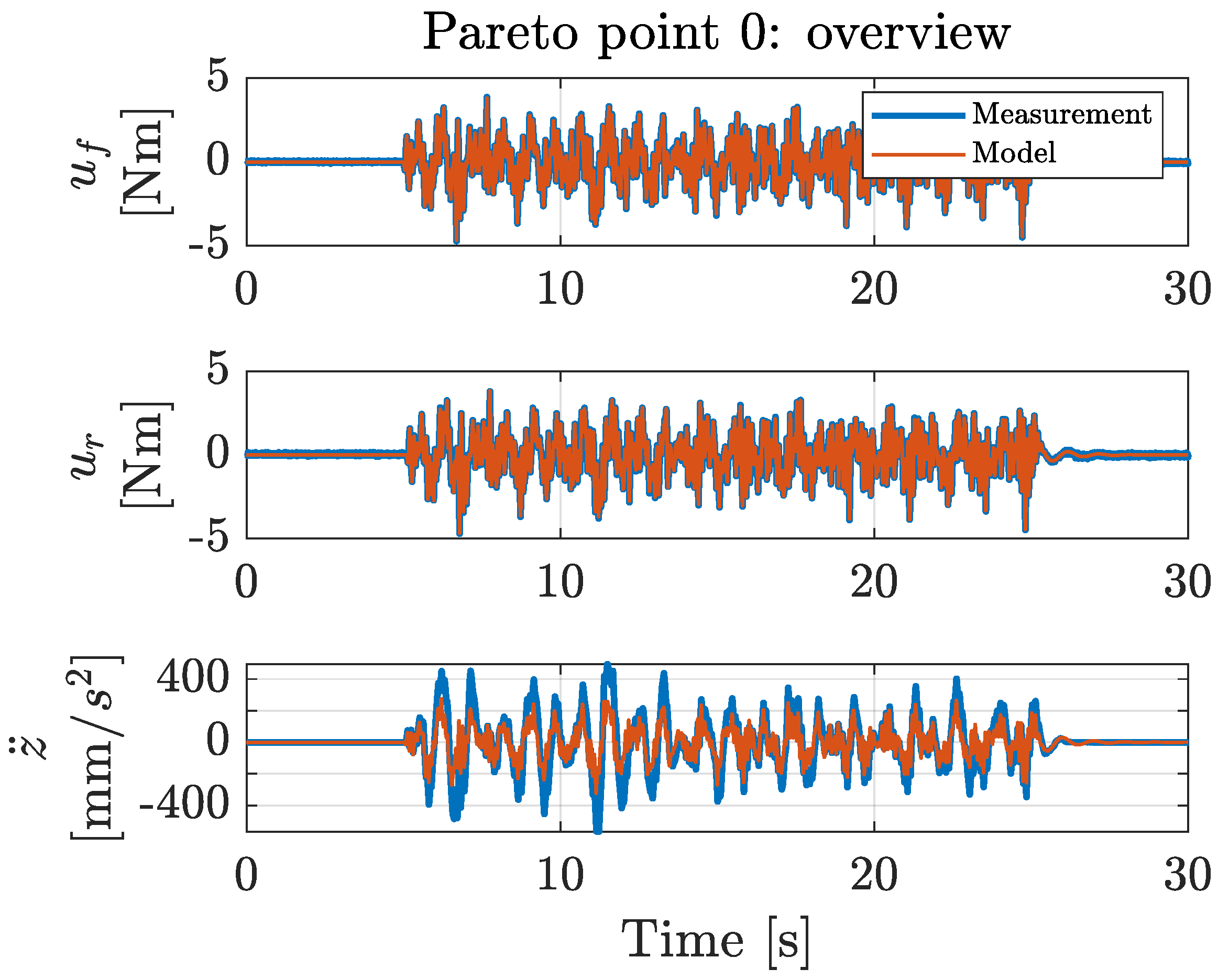
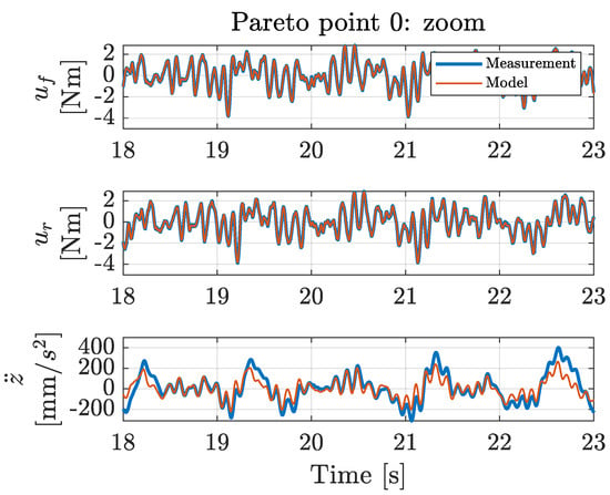
Figure A2.
Zoom from 18 to 23 s of the front wheel actuator output , rear wheel actuator output , and platform acceleration for the calculated model-based response (red) and the response measured in the physical setup (blue) for Pareto point 0.
Figure A2.
Zoom from 18 to 23 s of the front wheel actuator output , rear wheel actuator output , and platform acceleration for the calculated model-based response (red) and the response measured in the physical setup (blue) for Pareto point 0.
Appendix A.2. Pareto Point 1

Table A2.
Model-based Pareto front optimization results for Pareto point 1 (rounded).
Table A2.
Model-based Pareto front optimization results for Pareto point 1 (rounded).
| Pareto Point | Cost | Fitness Value | [, ... ] | [, ... ] | [, ... ] | [, ... ,] | [, ... ,] | [, ... ,] | [, ... ,] |
|---|---|---|---|---|---|---|---|---|---|
| 1 | 12.7 | 58,318 | [0, 1] | [0, 1] | [0, 1] | [0, 0, 0] | [0.040, 0.006, 0.009] | [0, 0, 0] | [0, 0, 0] |

Figure A3.
Overview of the front wheel actuator output , rear wheel actuator output , and platform acceleration for the calculated model-based response (red) and the response measured in the physical setup (blue) for Pareto point 1.
Figure A3.
Overview of the front wheel actuator output , rear wheel actuator output , and platform acceleration for the calculated model-based response (red) and the response measured in the physical setup (blue) for Pareto point 1.
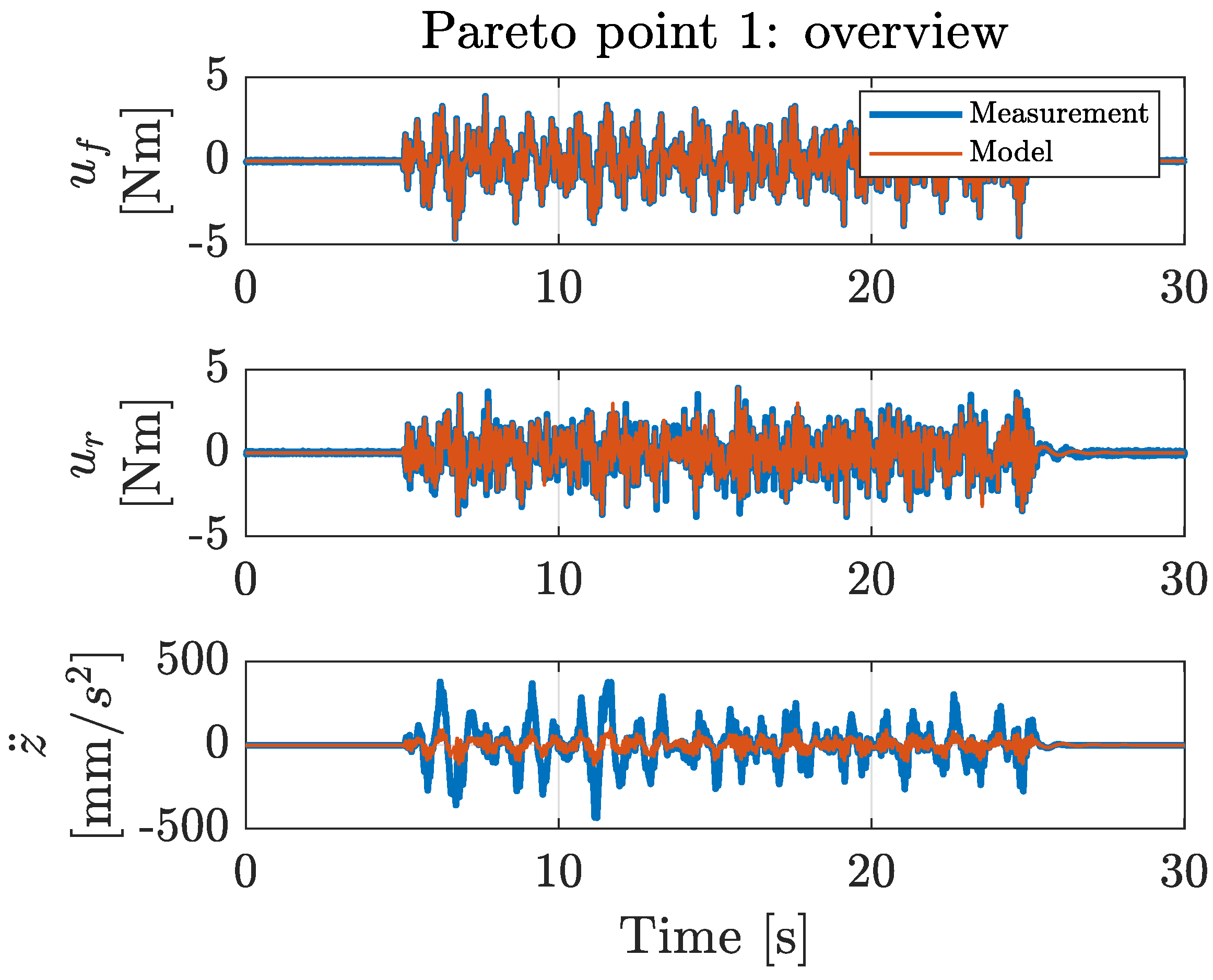

Figure A4.
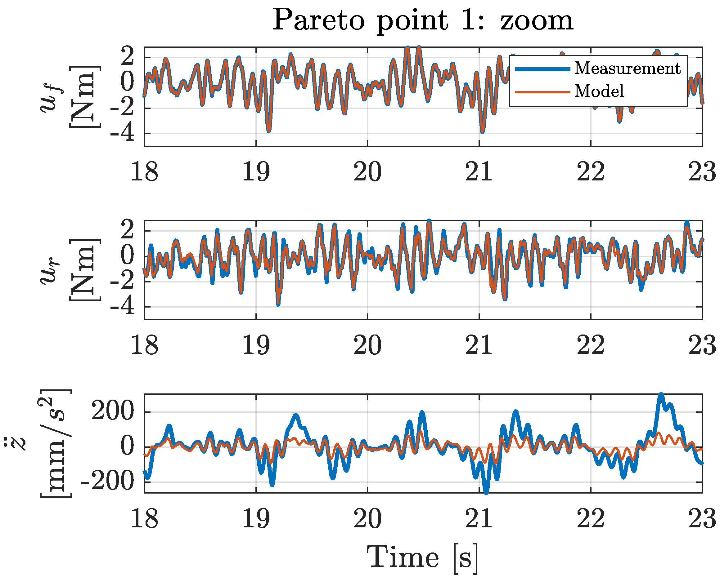
Zoom from 18 to 23 s of the front wheel actuator output , rear wheel actuator output , and platform acceleration for the calculated model-based response (red) and the response measured in the physical setup (blue) for Pareto point 1.
Figure A4.
Zoom from 18 to 23 s of the front wheel actuator output , rear wheel actuator output , and platform acceleration for the calculated model-based response (red) and the response measured in the physical setup (blue) for Pareto point 1.
Appendix A.3. Pareto Point 2

Table A3.
Model-based Pareto front optimization results for Pareto point 2 (rounded).
Table A3.
Model-based Pareto front optimization results for Pareto point 2 (rounded).
| Pareto Point | Cost | Fitness Value | [, ... ] | [, ... ] | [, ... ] | [, ... ,] | [, ... ,] | [, ... ,] | [, ... ,] |
|---|---|---|---|---|---|---|---|---|---|
| 2 | 18.7 | 36,633 | [1, 1] | [0, 1] | [0, 1] | [0.042, 0.003, 0.008] | [0.048, 0.001, 0.009] | [0, 0, 0] | [0, 0, 0] |

Figure A5.
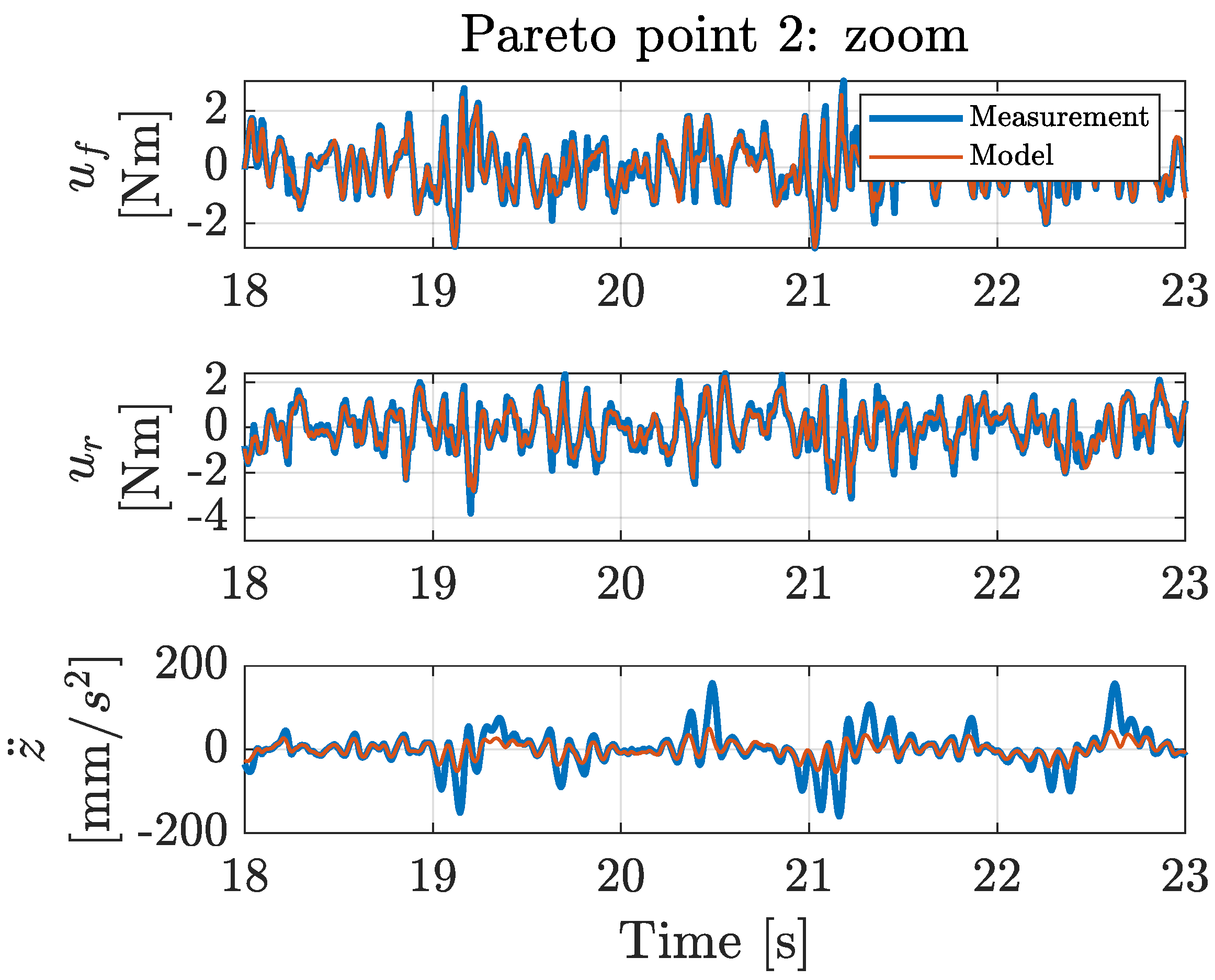
Overview of the front wheel actuator output , rear wheel actuator output , and platform acceleration for the calculated model-based response (red) and the response measured in the physical setup (blue) for Pareto point 2.
Figure A5.
Overview of the front wheel actuator output , rear wheel actuator output , and platform acceleration for the calculated model-based response (red) and the response measured in the physical setup (blue) for Pareto point 2.
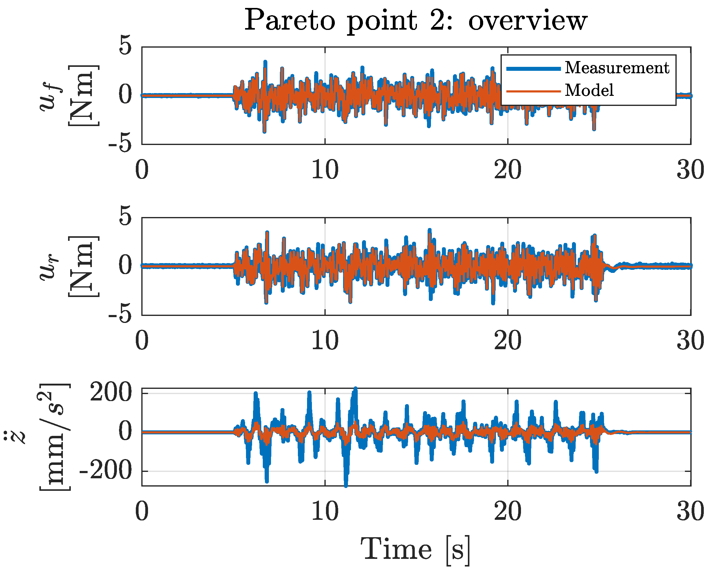

Figure A6.
Zoom from 18 to 23 s of the front wheel actuator output , rear wheel actuator output , and platform acceleration for the calculated model-based response (red) and the response measured in the physical setup (blue) for Pareto point 2.
Figure A6.
Zoom from 18 to 23 s of the front wheel actuator output , rear wheel actuator output , and platform acceleration for the calculated model-based response (red) and the response measured in the physical setup (blue) for Pareto point 2.
Appendix A.4. Pareto Point 3

Table A4.
Model-based Pareto front optimization results for Pareto point 3 (rounded).
Table A4.
Model-based Pareto front optimization results for Pareto point 3 (rounded).
| Pareto Point | Cost | Fitness Value | [, ... ] | [, ... ] | [, ... ] | [, ... ,] | [, ... ,] | [, ... ,] | [, ... ,] |
|---|---|---|---|---|---|---|---|---|---|
| 3 | 27.6 | 26,795 | [1, 2] | [0, 1] | [0, 1] | [0.043, 0.005, 0.004] | [0.036, 0.007, 0.007] | [0, 0, 0] | [0, 0, 0] |
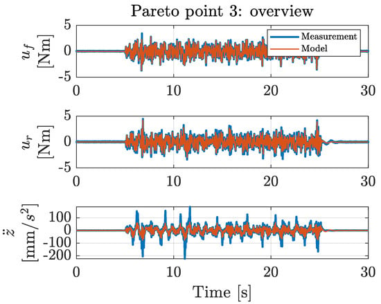
Figure A7.
Overview of the front wheel actuator output , rear wheel actuator output , and platform acceleration for the calculated model-based response (red) and the response measured in the physical setup (blue) for Pareto point 3.
Figure A7.
Overview of the front wheel actuator output , rear wheel actuator output , and platform acceleration for the calculated model-based response (red) and the response measured in the physical setup (blue) for Pareto point 3.
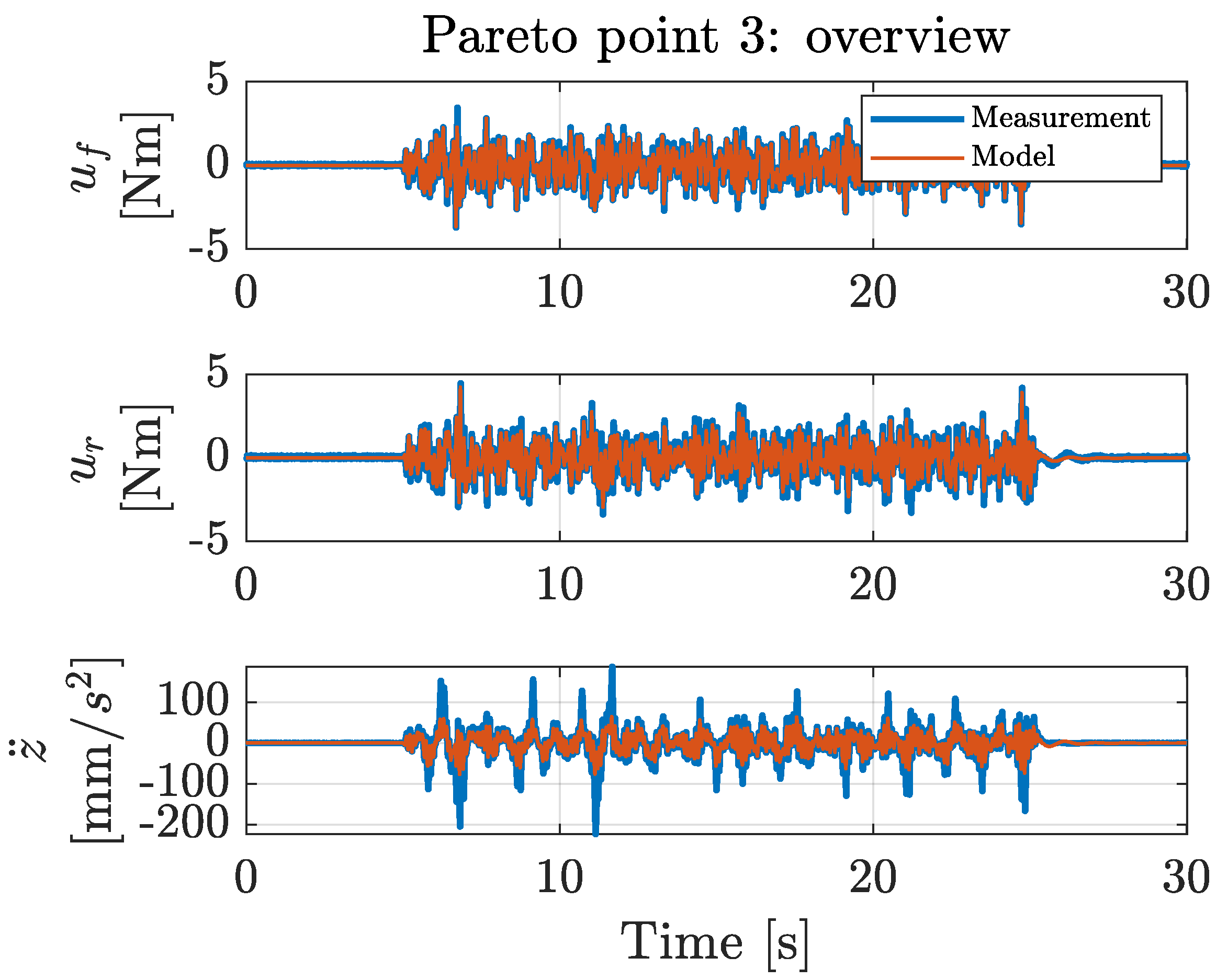
Figure A8.
Zoom from 18 to 23 s of the front wheel actuator output , rear wheel actuator output , and platform acceleration for the calculated model-based response (red) and the response measured in the physical setup (blue) for Pareto point 3.
Figure A8.
Zoom from 18 to 23 s of the front wheel actuator output , rear wheel actuator output , and platform acceleration for the calculated model-based response (red) and the response measured in the physical setup (blue) for Pareto point 3.
Appendix A.5. Pareto Point 4

Table A5.
Model-based Pareto front optimization results for Pareto point 4 (rounded).
Table A5.
Model-based Pareto front optimization results for Pareto point 4 (rounded).
| Pareto Point | Cost | Fitness Value | [, ... ] | [, ... ] | [, ... ] | [, ... ,] | [, ... ,] | [, ... ,] | [, ... ,] |
|---|---|---|---|---|---|---|---|---|---|
| 4 | 36.6 | 17,800 | [3, 2] | [0, 1] | [0, 1] | [0.049, 0.09, 0.003] | [0.049, 0.007, 0.008] | [0, 0, 0] | [0, 0, 0] |

Figure A9.
Overview of the front wheel actuator output , rear wheel actuator output , and platform acceleration for the calculated model-based response (red) and the response measured in the physical setup (blue) for Pareto point 4.
Figure A9.
Overview of the front wheel actuator output , rear wheel actuator output , and platform acceleration for the calculated model-based response (red) and the response measured in the physical setup (blue) for Pareto point 4.
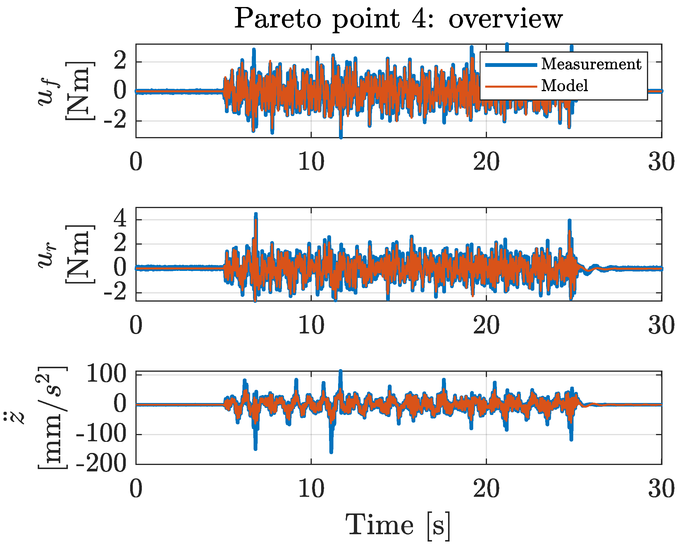
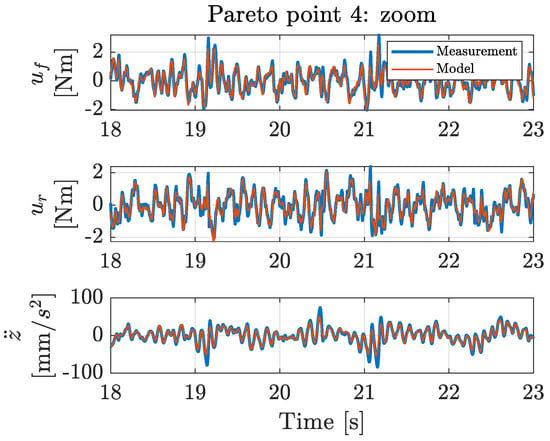
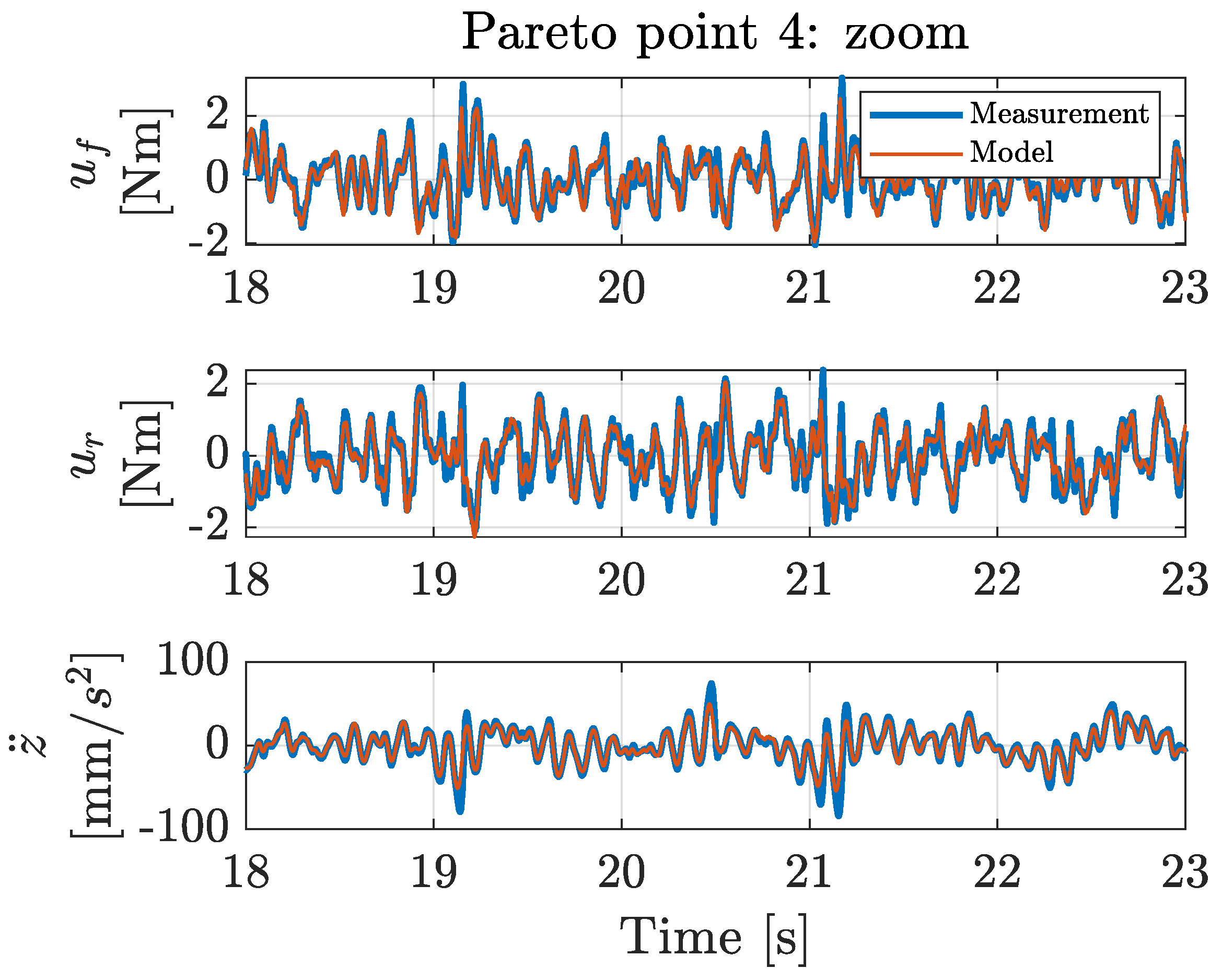
Figure A10.
Zoom from 18 to 23 s of the front wheel actuator output , rear wheel actuator output , and platform acceleration for the calculated model-based response (red) and the response measured in the physical setup (blue) for Pareto point 4.
Figure A10.
Zoom from 18 to 23 s of the front wheel actuator output , rear wheel actuator output , and platform acceleration for the calculated model-based response (red) and the response measured in the physical setup (blue) for Pareto point 4.
Appendix A.6. Pareto Point 5

Table A6.
Model-based Pareto front optimization results for Pareto point 5 (rounded).
Table A6.
Model-based Pareto front optimization results for Pareto point 5 (rounded).
| Pareto Point | Cost | Fitness Value | [, ... ] | [, ... ] | [, ... ] | [, ... ,] | [, ... ,] | [, ... ,] | [, ... ,] |
|---|---|---|---|---|---|---|---|---|---|
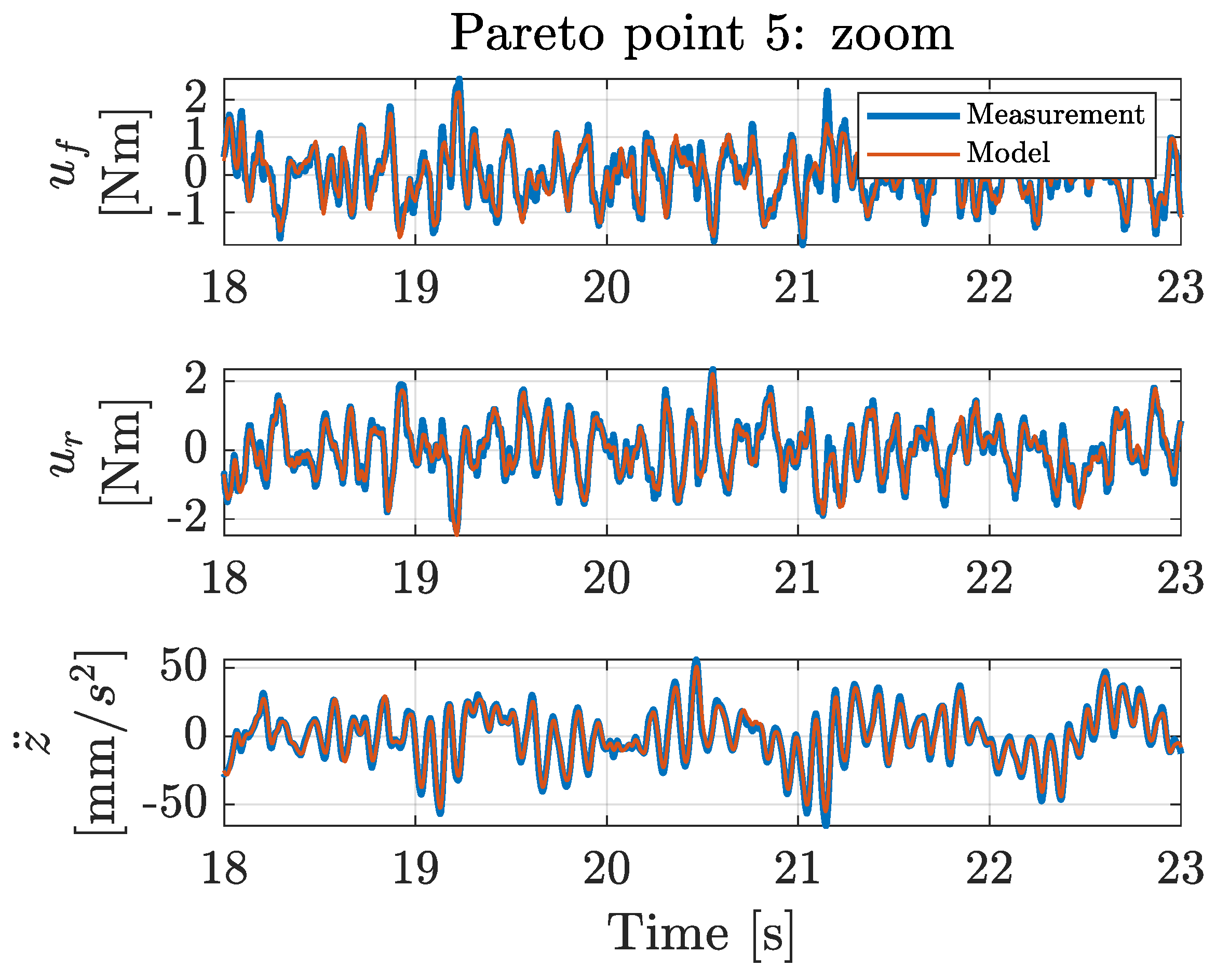
| 5 | 66.4 | 16,332 | [2, 2] | [0, 1] | [0, 1] | [0.048, 0.009, 0.009] | [0.043, 0.004, 0.007] | [0, 0, 0] | [0, 0, 0] |

Figure A11.
Overview of the front wheel actuator output , rear wheel actuator output , and platform acceleration for the calculated model-based response (red) and the response measured in the physical setup (blue) for Pareto point 5.
Figure A11.
Overview of the front wheel actuator output , rear wheel actuator output , and platform acceleration for the calculated model-based response (red) and the response measured in the physical setup (blue) for Pareto point 5.
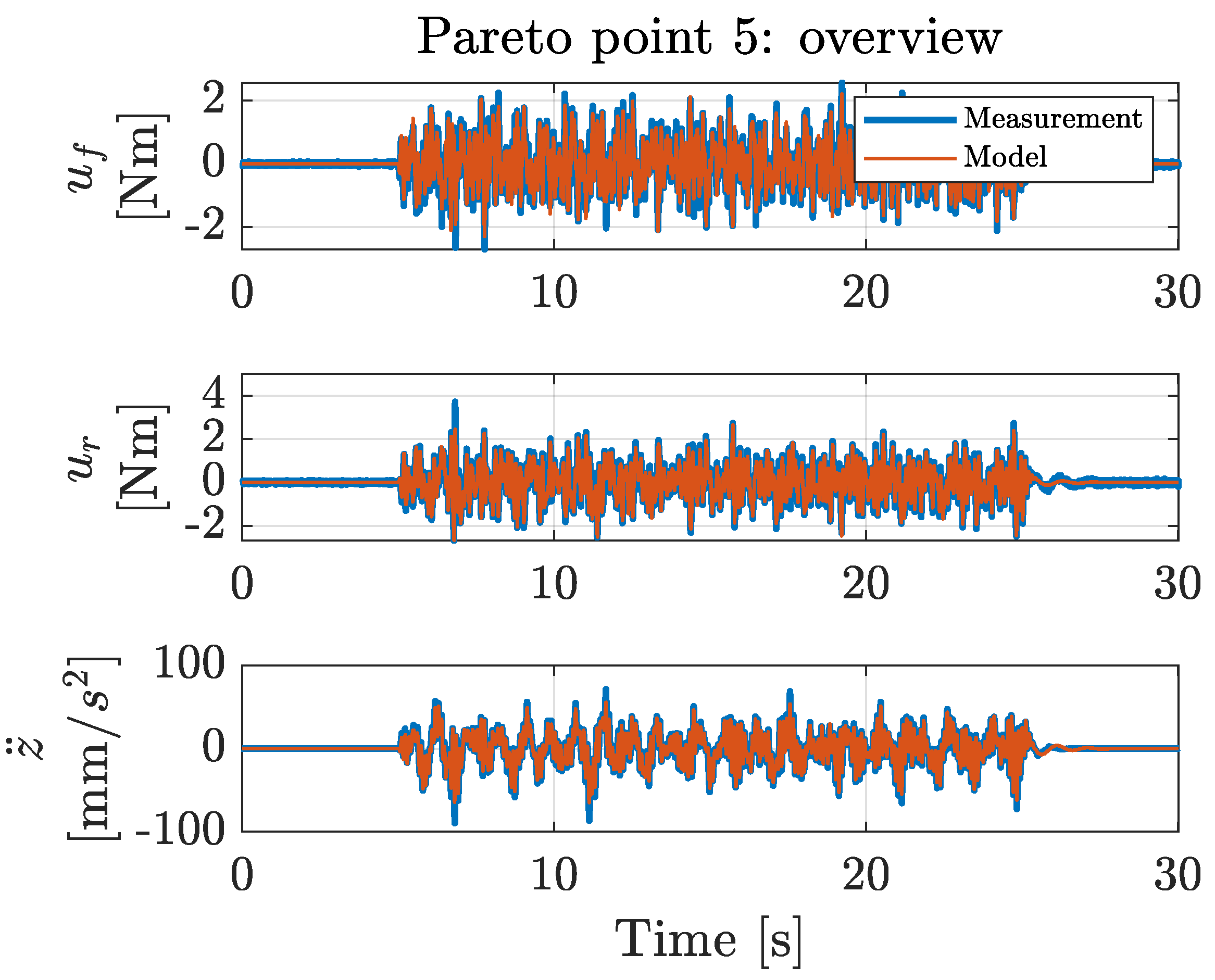
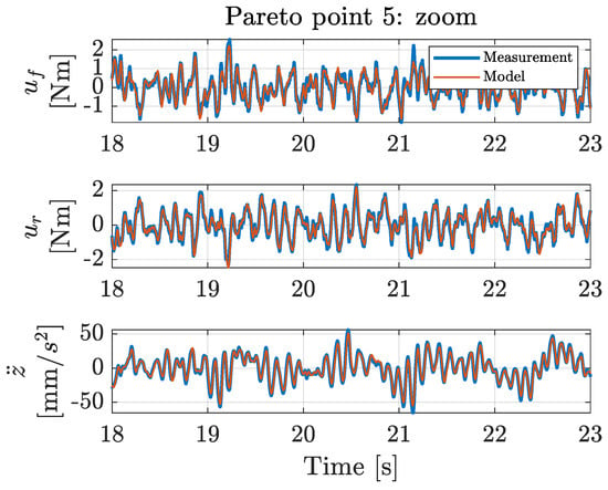
Figure A12.
Zoom from 18 to 23 s of the front wheel actuator output , rear wheel actuator output , and platform acceleration for the calculated model-based response (red) and the response measured in the physical setup (blue) for Pareto point 5.
Figure A12.
Zoom from 18 to 23 s of the front wheel actuator output , rear wheel actuator output , and platform acceleration for the calculated model-based response (red) and the response measured in the physical setup (blue) for Pareto point 5.
Appendix A.7. Pareto Point 6

Table A7.
Model-based Pareto front optimization results for Pareto point 6 (rounded).
Table A7.
Model-based Pareto front optimization results for Pareto point 6 (rounded).
| Pareto Point | Cost | Fitness Value | [, ... ] | [, ... ] | [, ... ] | [, ... ,] | [, ... ,] | [, ... ,] | [, ... ,] |
|---|---|---|---|---|---|---|---|---|---|
| 6 | 96.3 | 14,404 | [3, 3] | [0, 1] | [0, 1] | [0.05, 0, 0.01] | [0.05, 0.01, 0.01] | [0, 0, 0] | [0, 0, 0] |
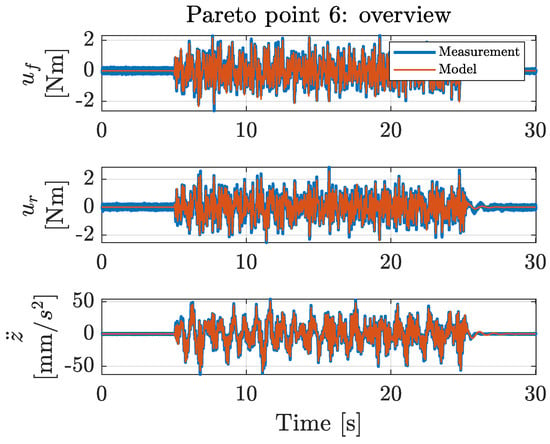
Figure A13.
Overview of the front wheel actuator output , rear wheel actuator output , and platform acceleration for the calculated model-based response (red) and the response measured in the physical setup (blue) for Pareto point 6.
Figure A13.
Overview of the front wheel actuator output , rear wheel actuator output , and platform acceleration for the calculated model-based response (red) and the response measured in the physical setup (blue) for Pareto point 6.
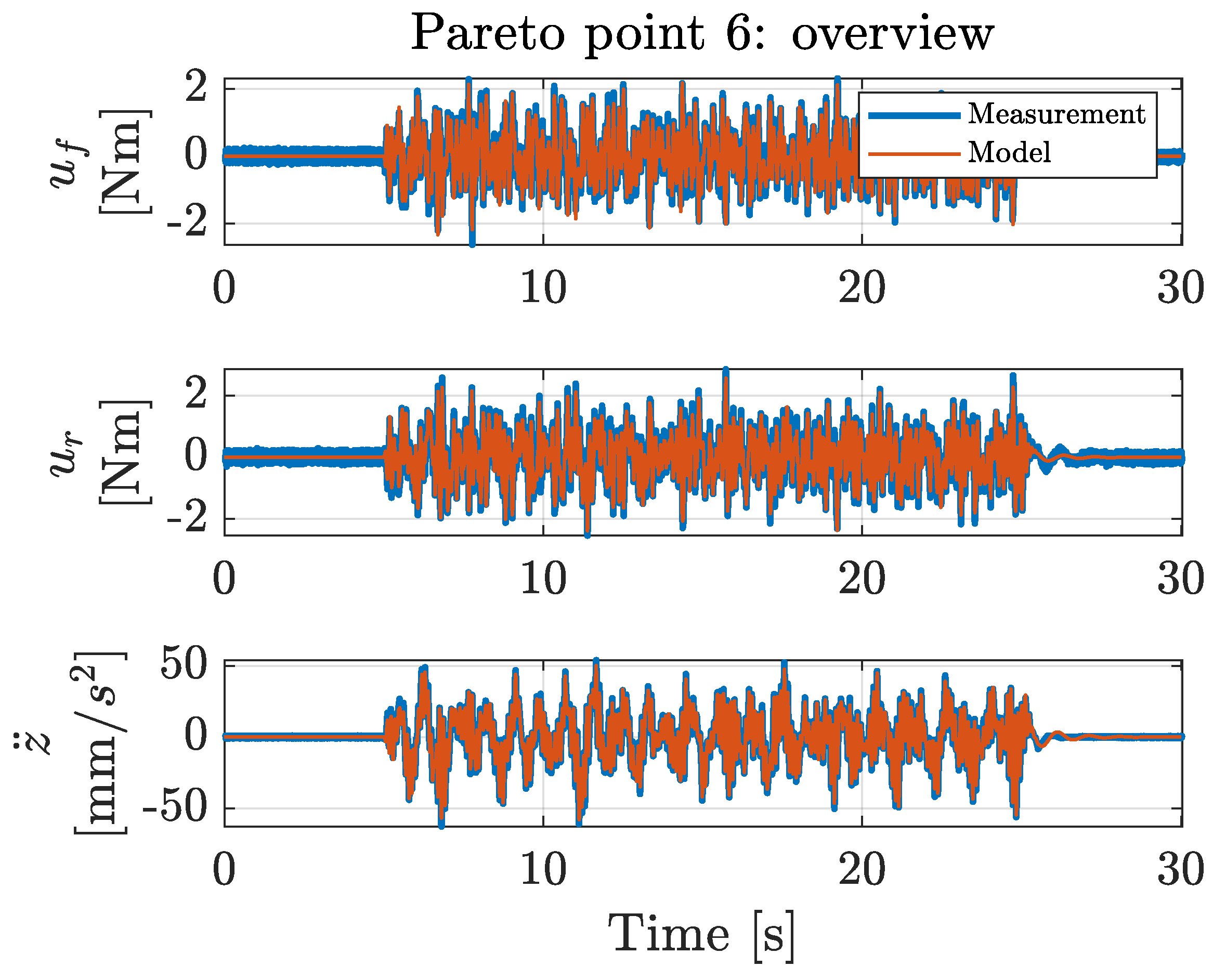
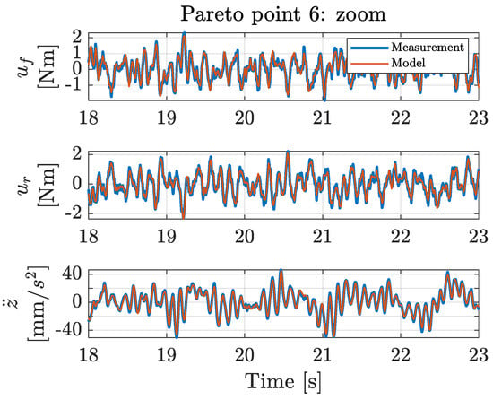
Figure A14.
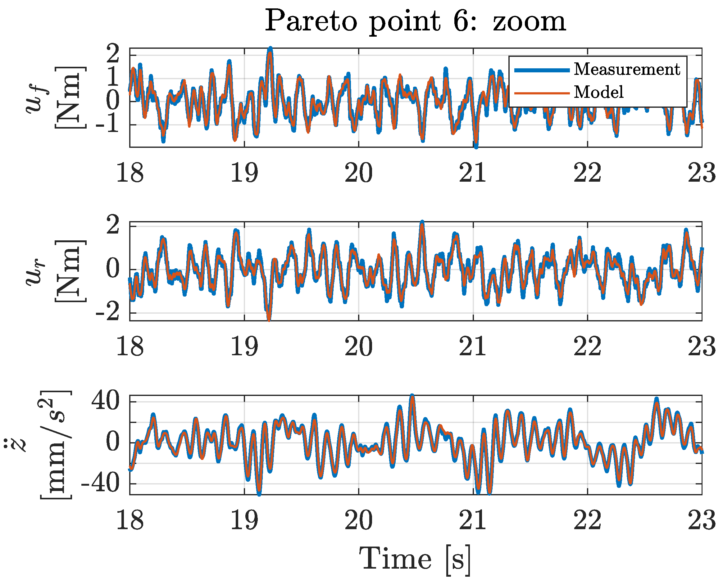
Zoom from 18 to 23 s of the front wheel actuator output , rear wheel actuator output , and platform acceleration for the calculated model-based response (red) and the response measured in the physical setup (blue) for Pareto point 6.
Figure A14.
Zoom from 18 to 23 s of the front wheel actuator output , rear wheel actuator output , and platform acceleration for the calculated model-based response (red) and the response measured in the physical setup (blue) for Pareto point 6.
References
- Roy, D.; Zhang, L.; Chang, W.; Chakraborty, S. Automated synthesis of cyber-physical systems from joint controller/architecture specifications. In Forum on Specification and Design Languages (FDL); IEEE: Bremen, Germany, 2016; pp. 1–8. [Google Scholar]
- Affi, Z.; EL-Kribi, B.; Romdhane, L. Advanced mechatronic design using a multi-objective genetic algorithm optimization of a motor-driven four-bar system. Mechatronics 2007, 17, 489–500. [Google Scholar] [CrossRef]
- Villarreal-Cervantes, M.G. Approximate and Widespread Pareto Solutions in the Structure-Control Design of Mechatronic Systems. J. Optim. Theory Appl. 2017, 173, 628–657. [Google Scholar] [CrossRef]
- Chen, C.Y.; Cheng, C.C. Integrated design for a mechatronic feed drive system of machine tools. In Proceedings of the IEEE ASME International Conference on Advanced Intelligent Mechatronics, Monterey, CA, USA, 24–28 July 2005; Volume 1, pp. 588–593. [Google Scholar]
- Moradi, M.; Naraghi, M.; Kamali Eigoli, A. Optimal codesign of controller and linear plants with input saturation: The sensitivity Lyapunov approach. Optim. Control. Appl. Methods 2018, 39, 622–637. [Google Scholar] [CrossRef]
- Chanekar, P.V.; Chopra, N.; Azarm, S. Co-design of linear systems using Generalized Benders Decomposition. Automatica 2018, 89, 180–193. [Google Scholar] [CrossRef]
- Fathy, H.K.; Reyer, J.A.; Papalambros, P.Y.; Ulsoy, A.G. On the coupling between the plant and controller optimization problems. In Proceedings of the American Control Conference, Arlington, VA, USA, 25–27 June 2001; Volume 3, pp. 1864–1869. [Google Scholar]
- Baheri, A.; Vermillion, C. Combined Plant and Controller Design Using Batch Bayesian Optimization: A Case Study in Airborne Wind Energy Systems. J. Dyn. Syst. Meas. Control. Trans. ASME 2019, 141, 091013. [Google Scholar] [CrossRef]
- Wang, Y.S.; Wang, Y. A gradient-based approach for optimal plant controller co-design. In Proceedings of the American Control Conference, Chicago, IL, USA, 1–3 July 2015; pp. 3249–3254. [Google Scholar]
- Ma, J.; Chen, S.L.; Teo, C.S.; Tay, A.; Al Mamun, A.; Tan, K.K. Parameter space optimization towards integrated mechatronic design for uncertain systems with generalized feedback constraints. Automatica 2019, 105, 149–158. [Google Scholar] [CrossRef]
- Reyer, J.A.; Papalambros, P.Y. Optimal Design and Control of an Electric DC Motor. In Proceedings of the ASME Design Engineering Technical Conferences, Las Vegas, NV, USA, 12–16 September 1999; pp. 1–12. [Google Scholar]
- Chen, Q.; Lin, T.; Ren, H. Parameters optimization and control strategy of power train systems in hybrid hydraulic excavators. Mechatronics 2018, 56, 16–25. [Google Scholar] [CrossRef]
- Haemers, M.; Derammelaere, S.; Rosich, A.; Ionescu, C.M.; Stockman, K. Towards a generic optimal co-design of hardware architecture and control configuration for interacting subsystems. Mechatronics 2019, 63, 102275. [Google Scholar] [CrossRef]
- Goldberg, D.E. Genetic Algorithms in Search, Optimization, and Machine Learning, 1st ed.; Addison-Wesley Publishing Company, Inc.: Reading, MA, USA, 1989. [Google Scholar]
- Wu, B.; Liu, C.; Song, X.; Wang, X. Design and implementation of the inverted pendulum optimal controller based on hybrid genetic algorithm. In Proceedings of the 2015 International Conference on Automation, Mechanical Control and Computational Engineering, Ji’nan, China, 24–26 April 2015; pp. 1480–1486. [Google Scholar]
- Du, H.; Lam, J.; Sze, K.Y. Non-fragile output feedback Hinfinity vehicle suspension control using genetic algorithm. Eng. Appl. Artif. Intell. 2003, 16, 667–680. [Google Scholar] [CrossRef]
- Haemers, M.; Derammelaere, S.; Ionescu, C.M.; Stockman, K.; De Viaene, J.; Verbelen, F. Proportional-Integral State-Feedback Controller Optimization for a Full-Car Active Suspension Setup using a Genetic Algorithm. IFAC Pap. 2018, 51, 1–6. [Google Scholar] [CrossRef]
- Van Oosterwyck, N.; Vanbecelaere, F.; Haemers, M.; Ceulemans, D.; Stockman, K.; Derammelaere, S. CAD Enabled Trajectory optimization and Accurate Motion Control for Repetitive Tasks. In Proceedings of the IEEE International Conference on Control and Automation (ICCA), Edinburgh, UK, 16–19 July 2019; pp. 387–392. [Google Scholar]
- Wang, H.; Mustafa, G.I.; Tian, Y. Model-free fractional-order sliding mode control for an active vehicle suspension system. Adv. Eng. Softw. 2018, 115, 452–461. [Google Scholar] [CrossRef]
- Nagarkar, M.; Vikhe Patil, G.J. Optimization of the linear quadratic regulator (LQR) control quarter car suspension system using genetic algorithm. Rev. Ing. E Investig. 2016, 36, 23–30. [Google Scholar] [CrossRef]
- Duc, G. Designing a Low Order Robust Controller for an Active Suspension System Thank LMI, Genetic Algorithm and Gradient Search. Eur. J. Control. 2003, 9, 29–38. [Google Scholar]
- Nagarkar, M.P.; El-Gohary, M.A.; Bhalerao, Y.J.; Vikhe Patil, G.J.; Zaware Patil, R.N. Artificial neural network predication and validation of optimum suspension parameters of a passive suspension system. SN Appl. Sci. 2019, 1, 1–17. [Google Scholar] [CrossRef]
- Baumal, A.; McPhee, J.; Calamai, P. Application of genetic algorithms to the design optimization of an active vehicle suspension system. Comput. Methods Appl. Mech. Eng. 1998, 163, 87–94. [Google Scholar] [CrossRef]
- Reza, J.N. Vehicle Dynamics: Theory and Application, 3rd ed.; Springer International Publishing: Berlin/Heidelberg, Germany, 2017. [Google Scholar]
- Alenezi, A. Active Suspension Control based on a Full-Vehicle Model. J. Electr. Electron. Eng. IOSR JEEE 2014, 9, 6–18. [Google Scholar] [CrossRef]
- Kruczek, A.; Stribrsky, A. A full-car model for active suspension—Some practical aspects. In Proceedings of the IEEE International Conference on Mechatronics, Istanbul, Turkey, 5 June 2004; IEEE: Istanbul, Turkey, 2004; pp. 41–45. [Google Scholar]
- Darus, R.; Sam, Y.M. Modeling and control active suspension system for a full car model. In Proceedings of the 5th the International Colloquium on Signal Processing Its Applications, Kuala Lumpur, Malaysia, 6–8 March 2009; Volume 4, pp. 13–18. [Google Scholar]
- Sharma, S.; Pare, V.; Chouksey, M.; Rawal, B. Numerical Studies Using Full Car Model for Combined Primary and Cabin Suspension. Procedia Technol. 2016, 23, 171–178. [Google Scholar] [CrossRef]
- Moradi, M.; Fekih, A. Adaptive PID-Sliding-Mode Fault-Tolerant Control Approach for Vehicle Suspension Systems Subject to Actuator Faults. IEEE Trans. Veh. Technol. 2014, 63, 1041–1054. [Google Scholar] [CrossRef]
- Ghosh, A. Scaling Laws. In Mechanics Over Micro and Nano Scales; Springer: New York, NY, USA, 2011; pp. 61–94. [Google Scholar]
- Verbandt, M.; Jacobs, L.; Turk, D.; Singh, T.; Swevers, J.; Pipeleers, G. Linear Control Toolbox—supporting B-splines in LPV control. Mechatronics 2018, 52, 78–89. [Google Scholar] [CrossRef]
- Ljung, L. Identification: Theory for the User, 2nd ed.; Prentice-Hall: Englewood Cliffs, NJ, USA, 1999; p. 607. [Google Scholar]
- ISO:8608-2016. Mechanical Vibration—Road Surface Profiles—Reporting of Measured Data, 2nd ed.; International Organization for Standardization: Vernier/Geneva, Switzerland, 2016; pp. 1–36. [Google Scholar]
- Tyan, F.; Hong, Y.F.; Tu, S.H.; Jeng, W.S. Generation of random road profiles. J. Adv. Eng. 2009, 4, 151–156. [Google Scholar]
- ISO:2631-2018. Mechanical Vibration and Shock—Evaluation of Human Exposure to Whole-Body Vibration—Part 5: Method for Evaluation of Vibration Containing Multiple Shocks, 2nd ed.; International Organization for Standardization: Vernier/Geneva, Switzerland, 2018; pp. 1–33. [Google Scholar]
- Skogestad, S.; Postlethwaite, I. Multivariable Feedback Control—Analysis and Design, 2nd ed.; John Wiley & Sons: Hoboken, NJ, USA, 2001. [Google Scholar]
- Kucukkoc, I.; Karaoglan, A.D.; Yaman, R. Using response surface design to determine the optimal parameters of genetic algorithm and a case study. Int. J. Prod. Res. 2013, 51, 5039–5054. [Google Scholar] [CrossRef]
- Gutowski, M. Biology, Physics, Small Worlds and Genetic Algorithms. In Leading Edge Computer Science Research; Nova Science Publishers, Inc.: Hauppauge, NY, USA, 2005; pp. 165–218. [Google Scholar]
- The MathWorks Inc. MATLAB Global Optimization Toolbox User’s Guide (Release 2018b); The MathWorks Inc.: Natick, MA, USA, 2018. [Google Scholar]
- Robandi, I.; Nishimori, K.; Nishimura, R.; Ishihara, N. Optimal feedback control design using genetic algorithm in multimachine power system. Int. J. Electr. Power Energy Syst. 2001, 23, 263–271. [Google Scholar] [CrossRef]
- Diaz-Rodriguez, I.D.; Bhattacharyya, S.P. PI controller design in the achievable gain-phase margin plane. In Proceedings of the 2016 IEEE 55th Conference on Decision and Control, CDC 2016, Las Vegas, NV, USA, 12–14 December 2016; pp. 4919–4924. [Google Scholar]
- Dorf, R.C.; Bishop, R.H. Modern Control Systems, 12th ed.; Prentice-Hall: Upper Saddle River, NJ, USA, 2011. [Google Scholar]
Publisher’s Note: MDPI stays neutral with regard to jurisdictional claims in published maps and institutional affiliations. |
© 2021 by the authors. Licensee MDPI, Basel, Switzerland. This article is an open access article distributed under the terms and conditions of the Creative Commons Attribution (CC BY) license (http://creativecommons.org/licenses/by/4.0/).

