Review

Observational Imprints of Enhanced Scalar Power on Small Scales in Ultra Slow Roll Inflation and Associated Non-Gaussianities

by
H. V. Ragavendra
1,†,‡ and
L. Sriramkumar
2,*,†
1
Department of Physical Sciences, Indian Institute of Science Education and Research Kolkata, Mohanpur 741246, India
2
Centre for Strings, Gravitation and Cosmology, Department of Physics, Indian Institute of Technology Madras, Chennai 600036, India
*
Author to whom correspondence should be addressed.
These authors contributed equally to this work.
Current address: Raman Research Institute, C. V. Raman Avenue, Sadashivanagar, Bengaluru 560080, India.
Galaxies 2023, 11(1), 34; https://doi.org/10.3390/galaxies11010034
Submission received: 12 December 2022 / Revised: 7 February 2023 / Accepted: 8 February 2023 / Published: 15 February 2023

Abstract

:
The discovery of gravitational waves from merging binary black holes has generated considerable interest in examining whether these black holes could have a primordial origin. If a significant number of black holes have to be produced in the early universe, the primordial scalar power spectrum should have an enhanced amplitude on small scales, when compared to the COBE normalized values on the large scales that is strongly constrained by the anisotropies in the cosmic microwave background. In the inflationary scenario driven by a single, canonical scalar field, such power spectra can be achieved in models that permit a brief period of ultra slow roll inflation during which the first slow roll parameter decreases exponentially. In this review, we shall consider a handful of such inflationary models as well as a reconstructed scenario and examine the extent of formation of primordial black holes and the generation of secondary gravitational waves in these cases. We shall also discuss the strength and shape of the scalar bispectrum and the associated non-Gaussianity parameter that arise in such situations. We shall conclude with an outlook wherein we discuss the wider implications of the increased strengths of the non-Gaussianities on smaller scales.

1. Introduction

Without a doubt, the inflationary scenario is the most compelling paradigm for overcoming the horizon problem associated with the hot big bang model and for simultaneously providing a natural mechanism for generating the perturbations in the early universe (see, for example, the reviews [1,2,3,4,5,6,7,8,9,10]). The simplest of inflationary models involve a single, canonical scalar field governed by a smooth potential, which typically leads to a long enough epoch of slow roll inflation to overcome the horizon problem. The perturbations are induced by the quantum fluctuations associated with the scalar field and they are expected to turn classical during the later stages of inflation. The increasingly precise measurements of the anisotropies in the cosmic microwave background (CMB) over the last couple of decades has led to strong constraints on the primordial scalar and tensor power spectra on large scales, i.e., over the wave numbers 10 4 k 10 1 Mpc 1 . The observations by the Planck mission [11,12] and the BICEP/Keck telescopes [13] constrain the primordial scalar amplitude A S , the scalar spectral index n S , and the tensor-to-scalar ratio r at the pivot scale of k * = 0.05 Mpc 1 to be: A S = 2.1 × 10 9 (a value referred to as COBE normalization), n S = 0.9649 ± 0.0042 and r < 0.036 at 95% confidence. In addition to the constraints on the power spectra, the data from Planck have also led to bounds on the primordial scalar bispectrum, limiting the values of the corresponding non-Gaussianity parameters f NL . The Planck data constrain the values of the parameters associated with the local, equilateral and orthogonal shapes of the bispectrum to be: f NL local = 0.9 ± 5.1 , f NL equil = 26 ± 47 and f NL ortho = 38 ± 24 [14,15]. These constraints suggest that simple slow roll inflationary models which are consistent with the data at the level of power spectra are also consistent at the level of scalar bispectra [16,17].
In contrast to the CMB scales, the constraints on the primordial scalar power spectrum over the smaller scales are considerably weaker. With the detection of gravitational waves (GWs) from merging black hole binaries [18,19,20], there has been interest in the literature to examine if these black holes could have a cosmological origin [21,22,23,24,25]. It has been known earlier that, if the amplitude of the primordial perturbations at small scales are adequately high (when compared to the COBE normalized amplitude over the CMB scales that we mentioned above), then these perturbations can be expected to collapse and form black holes when they reenter the Hubble radius during the radiation and matter dominated epochs (for earlier discussions, see, for example, Refs. [26,27,28]; also see the recent reviews [29,30,31,32,33,34]). However, in simple models of inflation that permit only slow roll, the amplitude of the scalar power spectrum will remain roughly at (or less than) the COBE normalized value even at smaller scales. A strong departure from slow roll during the later stages of inflation is required in order to generate power spectra with an enhanced amplitude on smaller scales that can produce a significant number of primordial black holes (PBHs).
In this review, we shall focus on single field models of inflation driven by the canonical scalar field. In such cases, it has been shown that a short period of ultra slow roll inflation wherein the first slow roll parameter decreases exponentially results in increased scalar power over scales that leave the Hubble radius just prior to or during the epoch of ultra slow roll (for the original discussions, see Refs. [35,36]; in this regard, also see Refs. [37,38]; for recent efforts, see, for example, Refs. [39,40,41,42,43,44,45,46,47,48,49]). We should mention that though the first slow roll parameter remains small during the period of ultra slow roll, the second and higher order slow roll parameters turn large during the phase leading to strong departures from slow roll inflation. Interestingly, it is found that inflationary potentials that contain a (near) inflection point inevitably lead to a phase of ultra slow roll. Besides, it has been found that potentials wherein a bump or a dip is added by hand or those that simply contain a sharp change in slope can also lead to an epoch of ultra slow roll (in this regard, see, for example, Refs. [50,51,52]). If inflation has to be terminated after the period of ultra slow roll, the first slow roll parameter has to steadily rise towards unity. The rapid fall and a steady rise in the first slow roll parameter leads to a peak in the spectrum of curvature perturbations whose height is determined by the smallest value attained by the parameter. Moreover, in such situations, it can be established that the scalar power rises as k 4 before it reaches the peak in the spectrum (for discussions in this regard, see Refs. [53,54,55,56,57,58,59,60]). A large enough value for the peak in the scalar power spectrum (but less than unity to ensure that the perturbation theory remains valid) can produce copious amounts of PBHs that can, in principle, constitute all of cold dark matter today. We shall restrict our discussion in this review to inflationary models that contain a (near) inflection point in the potential and lead to an epoch of ultra slow roll.
Interestingly, one finds that, when the curvature perturbations are enhanced over small scales in order to lead to increased formation of PBHs, they also induce secondary GWs of significant amplitudes when these wave numbers reenter the Hubble radius during the radiation dominated epoch (for early discussions, see Refs. [61,62,63,64]; for recent discussions, see, for instance, Refs. [65,66,67,68,69]). In fact, depending on the amplitude and location of the peak in the spectrum of curvature perturbations, the induced GWs can be of strengths comparable to the sensitivities of the ongoing and forthcoming GW observatories (for a summary of the sensitivity curves and their updated versions, see Ref. [70] and the associated web-page). Moreover, recall that, in slow roll inflation, the non-Gaussianity parameter f NL that reflects the strength of the scalar bispectrum is of the order of the first slow roll parameter, which is typically O ( 10 2 ) or less (see, for example, Refs. [71,72,73]). However, when deviations from slow roll occur, the non-Gaussianities can be considerably larger (in this regard, see, for instance, Refs. [49,74,75,76,77,78]). The enhanced strengths of non-Gaussianities can play a crucial role on the extent of PBHs produced (for very early efforts in this context, see Refs. [79,80,81]; for recent discussions, see Refs. [51,82,83,84,85,86,87,88,89,90,91,92,93,94]) as well as the strengths of the induced GWs [95,96,97,98,99,100].
The plan of this review is as follows. In the following section, we shall initially arrive at the equations of motion governing the background and the perturbations using the Arnowitt-Deser-Misner (ADM) formalism [101]. We shall then go on to introduce a handful of inflationary models that contain a near inflection point which permit an epoch of ultra slow roll inflation. We shall first describe the evolution of the background in such situations. We shall then discuss the challenges that arise in ensuring that the scalar and tensor power spectra in these models are consistent with the CMB data on large scales and describe the manner in which the challenges can be overcome by reverse engineering the desired potentials. In Section 3 and Section 4, we shall discuss the formation of PBHs and the generation of secondary GWs (during the epoch of radiation domination) in the various models and scenario of interest. In Section 5, after highlighting a few points related to the third order action that governs the scalar bispectrum, we shall describe the procedure for numerically computing the scalar bispectrum. We shall then go on to present the scalar bispectrum and the associated non-Gaussianity parameter that arise in some of the models that we consider. Lastly, in Section 6, we shall conclude with an outlook wherein we discuss the wider implications of the enhanced levels of non-Gaussianities on small scales.
Before we proceed further, let us make a few clarifying remarks regarding the conventions that we shall follow and the notations that we shall use. We shall work with natural units such that = c = 1 and set the reduced Planck mass to be M Pl = 8 π G 1 / 2 . We shall adopt the signature of the metric to be ( , + , + , + ) . Note that Latin indices will represent the spatial coordinates, apart from k which will be reserved for denoting the wave number. Also, an overdot and an overprime will denote differentiation with respect to the cosmic and conformal time coordinates t and η , respectively. Moreover, a will denote the scale factor, and the quantities H = a ˙ / a and H = a H = a / a will represent the Hubble and the conformal Hubble parameters. Further, N will represent the number of e-folds, which is defined through the relation d N / d t = H . A subscript N will denote the differentiation with respect to the number of e-folds. Lastly, we shall denote the canonical scalar field that we shall consider as ϕ , and a subscript ϕ will represent differentiation with respect to the scalar field.

2. Inflationary Models, Power Spectra and Reverse Engineered Potentials

In this section, we shall consider inflation driven by a canonical scalar field and first discuss the equations governing the background and the perturbations at the linear order. In contrast to the more common approach of using the zeroth and first order Einstein’s equations to arrive at the governing equations, we shall arrive at the equations using the ADM formalism [101]. As we shall see later, the approach proves to be helpful when we discuss the scalar bispectrum generated in the models of our interest. We shall then go on to introduce a handful of inflationary models that lead to an epoch of ultra slow roll inflation and discuss the scalar and tensor power spectra that arise in the models. We shall illustrate that, in these models, if we desire a sufficiently large peak in the power spectrum at small scales, there arises a challenge in ensuring that the scalar and tensor power spectra are consistent with the constraints from the CMB on large scales. In order to circumvent this difficulty, we shall discuss the method of reverse engineering desired potentials from a specific form of the first slow roll parameter.

2.1. Arriving at the Equations Governing the Background and the Perturbations at the Linear Order

As we mentioned, to arrive at the equations of motion governing the background and the perturbations, we shall make use of the ADM formalism [101]. Recall that, in the ADM formalism, the spacetime metric is expressed in terms of the lapse function N , the shift vector N i and the spatial metric h i j as follows:
d s 2 = N 2 d x 0 2 + h i j N i d x 0 + d x i N j d x 0 + d x j ,
where x 0 and x i denote the time and the spatial coordinates, respectively. We shall assume that gravitation is described by Einstein’s general theory of relativity. Since we shall be focusing on the epoch of inflation (to calculate the primordial power and bi-spectra), we shall assume that gravitation is sourced by a canonical, minimally coupled, scalar field ϕ , which is described by the potential V ( ϕ ) . In such a case, the action describing the complete system consisting of gravitation and the scalar field can be written in terms of the metric variables N , N i and h i j and the field ϕ as follows (see, for instance, Refs. [71,72,73,76,102]):
S [ N , N i , h i j , ϕ ] = d x 0 d 3 x N h { M Pl 2 2 1 N 2 E i j E i j E 2 + ( 3 ) R + [ 1 2 N 2 0 ϕ 2 N i N 2 0 ϕ i ϕ + N i N j 2 N 2 i ϕ j ϕ 1 2 h i j i ϕ j ϕ V ( ϕ ) ] } ,
where 0 ϕ = ϕ / x 0 , h det . ( h i j ) and ( 3 ) R is the curvature associated with the spatial metric h i j . The quantity E i j is given by
E i j = 1 2 0 h i j i N j j N i ,
with E = h i j E i j . Note that the variation of the above action with respect to the Lagrange multipliers N and N i leads to the so-called Hamiltonian and momentum constraints, respectively. Upon solving the constraint equations and substituting the solutions back in the original action (2), we can arrive at the action governing the dynamical variables of interest up to a given order in the perturbations.

2.1.1. Equations of Motion Describing the Background and the Slow Roll Parameters

We shall assume the background to be the spatially flat, Friedmann-Lemaître-Robertson-Walker (FLRW) universe described by the following line element:
d s 2 = d t 2 + a 2 ( t ) d x 2 = a 2 ( η ) d η 2 + d x 2 ,
where, as we mentioned, t and η denote cosmic and conformal time coordinates. Since we shall be interested in the situation wherein the FLRW universe is dominated by the canonical scalar field ϕ described by the potential V ( ϕ ) , we can arrive at the action governing the scale factor a and the homogeneous scalar field ϕ upon substituting the above line-element in the ADM action (2). At the leading order—i.e., at the zeroth order, with N i set to zero and h i j = a 2 ( t ) δ i j —we find that the complete action describing the system is given by
S 0 [ ϕ ( t ) ] = d t d 3 x a 3 3 M Pl 2 H 2 N + ϕ ˙ 2 2 N V ( ϕ ) .
If we now vary this action with respect to the lapse function N , we arrive at the following constraint equation upon setting N eventually to unity:
H 2 = 1 3 M Pl 2 ϕ ˙ 2 2 + V ( ϕ ) ,
which is the first Friedmann equation. On varying the above action with respect to the scalar field (with N set to unity) leads to the equation of motion for the scalar field given by
ϕ ¨ + 3 H ϕ ˙ + V ϕ = 0 .
It is useful to note that the above two equations can be combined to arrive at the equation
H ˙ = ϕ ˙ 2 2 M Pl 2 .
The first slow roll parameter is defined as [1,2,3,4,5,6,7,8,9,10]
ϵ 1 = H ˙ H 2 = H N H = ϕ ˙ 2 2 H 2 M Pl 2 = ϕ N 2 2 M Pl 2 .
The higher order slow roll parameters are defined in terms of the first slow roll parameter ϵ 1 through the relations
ϵ n + 1 = d ln ϵ n d N
for n 1 . For instance, one can show that the second slow roll parameter can be written as
ϵ 2 = 2 ϕ N N ϕ N .
As we shall see, it is the first three slow roll parameters, viz. ϵ 1 , ϵ 2 , and ϵ 3 , that determine the amplitude and shape of the inflationary power spectrum and bispectrum.

2.1.2. Scalar and Tensor Perturbations, Equations of Motion, Quantization and Power Spectra

Let us now arrive at the action and the equations of motion governing the scalar and tensor perturbations using the ADM formalism. To do so, it turns out to be convenient if we choose to work in a particular gauge. We shall work in the so-called comoving gauge wherein the perturbation in the scalar field, say, δ ϕ , vanishes identically [71]. In other words, in the gauge of our choice, the scalar field ϕ depends only on time. Let the scalar perturbation be described by the curvature perturbation R and let the tensor perturbation be characterized by γ i j . On taking into account these perturbations, it is convenient to express the spatially flat FLRW metric (4) as [71]
d s 2 = d t 2 + a 2 ( t ) e 2 R ( t , x ) e γ ( t , x ) i j d x i d x j .
The assumption for the scalar field ϕ , the above form of the FLRW metric and the solutions to the Hamiltonian and momentum constraint equations allow us to arrive at the action describing the scalar and tensor perturbations R and γ i j at a given order [71,72,73]. It can be shown that, in the comoving gauge of interest, at the quadratic order, the actions governing the curvature perturbation R and the tensor perturbation γ i j can be expressed as [71,72,76,103]
S 2 [ R ( η , x ) ] = 1 2 d η d 3 x z 2 R 2 R 2 ,
S 2 [ γ i j ( η , x ) ] = M Pl 2 8 d η d 3 x a 2 γ i j 2 γ i j 2 ,
where z = a 2 ϵ 1 M Pl , with ϵ 1 being the first slow roll parameter. The above quadratic actions will evidently lead to linear equations of motion. In Fourier space, the modes functions, say, f k and g k , associated with the scalar and the tensor perturbations are found to satisfy the differential equations
f k + 2 z z f k + k 2 f k = 0 ,
g k + 2 a a g k + k 2 g k = 0 ,
respectively.
As we indicated earlier, in the inflationary paradigm, the primordial perturbations arise due to quantum fluctuations. On quantization, the scalar and tensor perturbations R and γ i j can be elevated to be quantum operators. The operators R ^ and γ ^ i j can be decomposed in terms of the corresponding mode functions f k and g k —which satisfy the equations of motion (14)—as follows:
R ^ ( η , x ) = d 3 k ( 2 π ) 3 / 2 R ^ k ( η ) e i k · x = d 3 k ( 2 π ) 3 / 2 a ^ k f k ( η ) e i k · x + a ^ k f k * ( η ) e i k · x ,                                                        
γ ^ i j ( η , x ) = d 3 k 2 π 3 / 2 γ ^ i j k ( η ) e i k · x = s d 3 k ( 2 π ) 3 / 2 b ^ k s ε i j s ( k ) g k ( η ) e i k · x + b ^ k s ε i j s * ( k ) g k * ( η ) e i k · x .
In the expression for the operator describing the tensor perturbations, the quantity ε i j s ( k ) represents the polarization tensor of the GWs with their helicity being denoted by the index s. Moreover, in the above decompositions, the two independent sets of operators ( a ^ k , a ^ k ) and ( b ^ k s , b ^ k s ) denote the annihilation and creation operators associated with the scalar and tensor modes corresponding to the wave vector k and helicity s (with the latter applying to the case of tensors). These operators are governed by the following, standard commutation relations:
[ a ^ k , a ^ k ] = [ a ^ k , a ^ k ] = 0 , [ a ^ k , a ^ k ] = δ ( 3 ) k k ,          
[ b ^ k s , b ^ k s ] = [ b ^ k s , b ^ k s ] = 0 , [ b ^ k s , b ^ k s ] = δ s s δ ( 3 ) k k .
Note that the transverse and traceless nature of GWs leads to the conditions δ i j k i ε j l s ( k ) = δ i j ε i j s ( k ) = 0 . We should point our that we shall work with the normalization condition δ i j δ l m ε i l r ( k ) ε j m s * ( k ) = 2 δ r s [71].
Often, it proves to be convenient to introduce the so-called Mukhanov-Sasaki variables to describe the scalar and tensor perturbations. These variables are defined as v k = z f k and u k = M Pl a g k / 2 and, in terms of these variables, the equations of motion (14) that govern the scalar and the tensor perturbations reduce to
v k + k 2 z z v k = 0 ,
u k + k 2 a a u k = 0 .
The scalar and the tensor power spectra, viz. P S ( k ) and P T ( k ) , are defined through the relations
R ^ k ( η e ) R ^ k ( η e ) = ( 2 π ) 2 2 k 3 P S ( k ) δ ( 3 ) ( k + k ) ,                  
γ ^ i j k ( η e ) γ ^ m n k ( η e ) = ( 2 π ) 2 2 k 3 Π i j , m n k 4 P T ( k ) δ ( 3 ) ( k + k ) ,
where the expectation values on the left hand sides are to be evaluated in the specified initial quantum state of the perturbations and η e is the conformal time at late times, close to the end of inflation. The quantity Π i j , m n k is given by [104]
Π i j , m n k = s ε i j s ( k ) ε m n s * ( k ) .
Typically, the expectation values are evaluated in the vacuum state, say, | 0 , associated with the quantized perturbations. The state satisfies the conditions a ^ k | 0 = 0 and b ^ k s | 0 = 0 for all wave numbers k and helicity s. The initial state is defined at very early times when all the scales of cosmological interest are well inside the Hubble radius during inflation and the quantum state is referred to as the Bunch-Davies vacuum [105]. The scalar and tensor power spectra P S ( k ) and P T ( k ) can be expressed in terms of the mode functions ( f k , g k ) and the associated Mukhanov-Sasaki variables ( v k , u k ) as follows:
P S ( k ) = k 3 2 π 2 | f k ( η e ) | 2 = k 3 2 π 2 | v k ( η e ) | 2 z 2 ( η e ) ,                              
P T ( k ) = 4 k 3 2 π 2 | g k ( η e ) | 2 = 8 M Pl 2 k 3 2 π 2 | u k ( η e ) | 2 a 2 ( η e ) .

2.2. A Short List of Models Permitting Ultra Slow Roll Inflation

A wide variety of models which permit an epoch of ultra slow roll inflation have been considered in the literature (for a short list of such efforts, see Refs. [39,40,41,42,43,44,45,46,47,48,49,106]). Curiously, many of these models contain a point of inflection, i.e., a point where the first and the second derivatives of the potential with respect to the scalar field (viz. V ϕ and V ϕ ϕ = d 2 V / d ϕ 2 ) vanish (in this regard, see Appendix A). We shall consider six of these models and we shall now briefly describe the models of our interest and the parameters that we shall work with. For convenience, in our discussions that follow, we shall refer to these models as M1 to M6. In the introductory section, we had mentioned that the CMB observations strongly constrain the scalar amplitude, the scalar spectral index and the tensor-to-scalar ratio at the pivot scale k * . We shall assume that the pivot scale leaves the Hubble radius N * number of e-folds before the end of inflation. We should point out that, in the absence of detailed modeling of post-inflationary dynamics, there arises some uncertainty in the choice of N * and it is often assumed to lie in the range 50 N * 60 [11,12,107].
  • Model 1: The first of the models that we shall consider, which leads to a period of ultra slow roll inflation, is described by a potential that can be written in the following fashion [39]:
    V ( ϕ ) = V 0 6 x 2 4 α x 3 + 3 x 4 ( 1 + β x 2 ) 2 ,
    where x = ϕ / v , with v being a constant. We shall work with the following choices for the four parameters that describe the potential: V 0 = 4 × 10 10 M Pl 4 , v = 0.108 M Pl , α = 1 and β = 1.4349 . For these values of the parameters, the (near) inflection point, say, ϕ 0 , is located at 0.39 M Pl . (For a discussion on the determination of the inflection points numerically in the inflationary models being considered, see Appendix A). If we choose the initial value of the field to be ϕ i = 3.614 M Pl and ϵ 1 i = 10 3 (which determines ϕ N i , cf. Equation (9)), we find that inflation lasts for about 63 e-folds in the model. Also, in this case, we shall set N * = 50 .
  • Model 2: The second potential that we shall consider can expressed in terms of the quantity x = ϕ / v that we had introduced in the first model, and is given by [46]
    V ( ϕ ) = V 0 α x 2 β x 4 + γ x 6 ( 1 + δ x 2 ) 2 .
    We shall consider the following set of values for the six parameters involved: V 0 = 1.3253 × 10 9 M Pl 4 , v = 10 M Pl , α = 8.53 × 10 2 , β = 0.458 , γ = 1 and δ = 1.5092 . For these values of the parameters and the initial conditions ϕ i = 17.245 M Pl and ϵ 1 i = 10 2 , inflation continues for about 75 e-folds before it is terminated. Also, the point of inflection is located at ϕ 0 = 1.72 M Pl . For this model, we shall choose N * = 55 .
  • Model 3: A potential referred to as the critical Higgs model is given by [42,43,47]:
    V ( ϕ ) = V 0 1 + a ln x 2 x 4 1 + c 1 + b ln x x 2 2 ,
    where x = ϕ / μ and we shall set μ = 1 M Pl . We shall choose the values of the other parameters that describe the potential to be V 0 = 7.05 × 10 8 M Pl 4 , a = 1.694 , b = 0.601 and c = 2.850 . For these values, the point of inflection occurs at ϕ 0 = 0.820 M Pl . The initial values of the field and the first slow roll parameter are taken to be ϕ i = 8.00 M Pl and ϵ 1 i = 10 3 . In such a case, we achieve about 103 e-folds of inflation. The pivot scale is set to exit the Hubble radius at about 70 e-folds before the end of inflation to achieve the feature at the desired wave number.
  • Model 4: The fourth potential that we shall consider is given by [45]
    V ( ϕ ) = V 0 tanh ϕ 6 M Pl + A sin tanh ϕ / 6 M Pl f ϕ 2
    and we shall work with the following values of the parameters involved: V 0 = 2 × 10 10 M Pl 4 , A = 0.130383 and f ϕ = 0.129576 . For these values of the parameters, we find that a point of inflection arises at ϕ 0 = 1.05 M Pl . If we set initial value of the field to be ϕ i = 6.1 M Pl and the first slow roll parameter to be ϵ 1 i = 10 3 , we obtain about 66 e-folds of inflation in the model. Also, we shall choose N * = 50 .
  • Model 5: A model constructed from supergravity which permits a period of ultra slow inflation is described by the potential [45,48]
    V ( ϕ ) = V 0 c 0 + c 1 tanh ϕ 6 α + c 2 tanh 2 ϕ 6 α + c 3 tanh 3 ϕ 6 α 2 .
    We shall work with the following values for the parameters involved: V 0 = 2.1 × 10 10 M Pl 4 , c 0 = 0.16401 , c 1 = 0.3 , c 2 = 1.426 , c 3 = 2.20313 and α = 1 M Pl 2 . This model too contains a point of inflection and, for the above values for the parameters, the inflection point is located at ϕ 0 = 0.53 M Pl . We find that, for the initial values ϕ i = 7.4 M Pl and ϵ 1 i = 10 3 , inflation ends after about 68 e-folds. Also, in this case, we shall set N * = 50 .
  • Model 6: The sixth and last model that we shall consider is motivated by string theory, and is described by the potential [44]
    V ( ϕ ) = W 0 2 V 3 { C up V 1 / 3 C W τ K 3 ( ϕ ) + A W τ K 3 ( ϕ ) B W + τ K 3 ( ϕ ) V D W G W 1 + ( R W / V ) τ K 3 3 / 2 ( ϕ ) } ,
    where τ K 3 ( ϕ ) = exp [ 2 ϕ / ( 3 M Pl ) , W 0 = 9.469 M Pl 2 , V = 10 3 , C up = 0 , C W = 0.04 , A W = 0.02 , B W = 1.00 , D W = 0 , G W = 3.081 × 10 5 V , and R W = 7.071 × 10 4 V . To achieve the required duration of inflation, we shall set ϕ i = 10.0 M Pl and ϵ 1 i = 2 × 10 3 . These initial conditions lead to about 68 e-folds of inflation. We shall set N * = 50 to compute the power spectra arising in the model.

2.3. Evolution of the Background in Ultra Slow Roll Inflation

We shall solve the equations of motion governing the background and the perturbations numerically to arrive at the scalar and tensor power spectra in a given inflationary model. To make the numerical computation efficient, as is usually done, we shall use the number of e-folds N as the independent time variable. Note that the first Friedmann Equation (6) and the equation of motion (7) can be combined to arrive at the following equation for the scalar field:
ϕ N N + 3 ϕ N 2 2 M Pl 2 ϕ N + 3 M Pl 2 ϕ N 2 2 V ϕ V = 0 .
Given the potential describing the scalar field, the values of the parameters and the initial conditions (viz. ϕ i and ϵ 1 i , with the latter determining ϕ N i ), we utilize the fifth order Runge-Kutta method, with an adaptive step size, to evolve the above equation [108,109]. Once the solution for the scalar field is at hand, all the other background quantities, including the slow roll parameters, can be expressed in terms of the scalar field and its time derivatives.
Let us now understand the evolution of the background in the inflationary models of interest. We can gain an overall perspective of the dynamics involved from the behavior of the field in the phase space ϕ - ϕ N . In Figure 1, we have presented the phase portrait of the scalar field for the two models M1 and M2. We should highlight three points regarding the figure. Firstly, it is clear that the trajectories with different initial conditions quickly merge with the primary trajectory of interest (viz. the one evolved from the initial conditions mentioned above). Secondly, independent of the initial conditions, the speed of the scalar field reduces considerably as it approaches the point of inflection. It is this behavior that is responsible for the epoch of ultra slow roll inflation in these models. In fact, we find that, around the point of inflection, certain trajectories with insufficient velocities may stagnate and not evolve beyond the point. Lastly, the slow roll approximation fails to capture the dynamics of the field near and beyond the point of inflection.
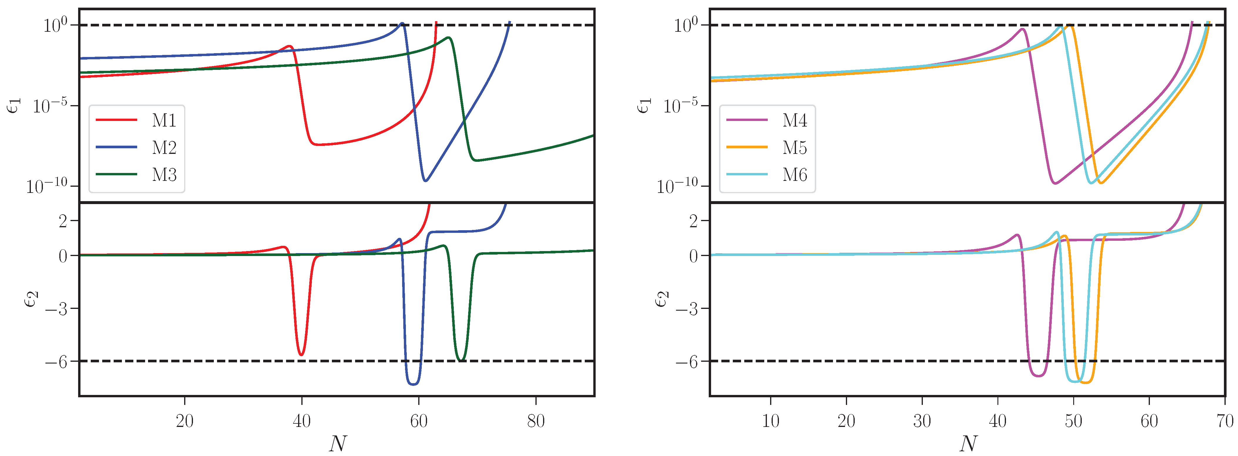
In Figure 2, we have plotted the evolution of the first two slow roll parameters in the six models M1 to M6. Note that all the models permit a short epoch wherein the first slow roll parameter ϵ 1 decreases rapidly and the second parameter ϵ 2 remains nearly a constant. In fact, from Equation (7), it is straightforward to establish that, when a slowly rolling field approaches a regime wherein V ϕ 0 , ϕ ˙ will begin to behave as a 3 . This implies that the first slow roll parameter behaves as ϵ 1 a 6 , thereby leading to ϵ 2 6 during the epoch. It should be clear from the figure that the first two slow roll parameters indeed roughly exhibit such a behavior during the epoch of ultra slow roll in all the models of interest. Interestingly, we find that, in some cases, inflation is briefly interrupted for about an e-fold or so (a scenario dubbed as punctuated inflation; in this context, see Refs. [49,110,111]) before the epoch of ultra slow roll sets in, and inflation is eventually terminated at a later stage when the first slow roll parameter crosses unity again.

2.4. Scalar and Tensor Power Spectra in Ultra Slow Roll Inflation

Let us now discuss the numerical evaluation of the scalar and tensor power spectra (in this context, see Refs. [49,77,78,112,113,114,115]). As in the case of the background, we shall work with e-folds N as the independent time variable. In such a case, the differential Equation (14) governing the perturbations can be expressed as follows:
f N N k + 3 ϵ 1 + ϵ 2 f N k + k a H 2 f k = 0 ,
                    g N N k + 3 ϵ 1 g N k + k a H 2 g k = 0 ,
where, for convenience, we have denoted ( f k , g k ) as ( f k , g k ) .
During inflation, the initial conditions on the perturbations are imposed when the physical wavelengths a / k are well inside the Hubble radius H 1 , i.e., when ( a H ) / k 1 or, equivalently, when k / ( a H ) 1 . In fact, to be precise, the conditions are to be imposed on the scalar and tensor perturbations when k z / z and k a / a , respectively [77,78]. It should be clear from Equation (17) that, in such a limit, the k 2 term will dominate and, as a result, the Mukhanov-Sasaki variables v k and u k will exhibit oscillatory behavior, i.e., they behave in the same manner as they would in Minkowski spacetime. Such a behavior should not be surprising. The quantities z / z and a / a roughly determine the scale of curvature of the inflationary background and the limits k z / z and k a / a correspond to the domain wherein the physical wavelengths are much smaller than the curvature scale. In such a domain, the initial conditions imposed on the Mukhanov-Sasaki variables v k and u k are given by
v k ( η i ) = u k ( η i ) = 1 2 k e i k η i ,      
v k ( η i ) = u k ( η i ) = i k 2 e i k η i ,
where η i denotes an adequately early time when the conditions are imposed. The vacuum state that is associated with such initial conditions is popularly known as the Bunch-Davies vacuum [105], as had mentioned earlier. In terms of the mode functions f k and g k , the above initial conditions correspond to
f k ( N i ) = 1 2 k z ( N i ) , f N k ( N i ) = 1 2 k z ( N i ) i k a ( N i ) H ( N i ) + z N ( N i ) z ( N i ) ,                              
g k ( N i ) = 2 M Pl 1 2 k a ( N i ) , g N k ( N i ) = 2 M Pl 1 2 k a ( N i ) i k a ( N i ) H ( N i ) + 1 .
where z N = d z / d N and we have dropped the overall and unimportant phase factor exp ( i k η i ) in all the expressions.
Numerically, one finds that it is often sufficient to impose the initial conditions when k 10 2 z / z and k 10 2 a / a on the scalar and tensor perturbations, respectively [49,77,78,112,113,114,115]. With the solutions to background at hand, we can evaluate the coefficients in the Equation (28) governing the perturbations. Starting with the initial conditions (30), we use the fifth order Runge-Kutta method [109] to evolve the scalar and tensor perturbations until late times. In simple scenarios involving slow roll inflation, the amplitudes of the modes quickly approach a constant value soon after they leave the Hubble radius. Therefore, typically, the spectrum of scalar and tensor perturbations are evaluated on super-Hubble scales, say, when k 10 5 z / z and k 10 5 a / a . However, in scenarios that permit a period of ultra slow roll, the amplitudes of the modes which leave the Hubble radius just prior to or during the epoch of ultra slow roll inflation can be affected even after they leave the Hubble radius1 Due to these reasons, in the models of our interest that lead to an epoch of ultra slow roll inflation, we evaluate the scalar and tensor power spectra close to the end of inflation, well past the epoch of ultra slow roll.
In Figure 3, we have plotted the scalar and tensor power spectra that arise in the models M1 to M6. While the power spectra are nearly scale invariant over large scales, clearly, the scalar spectra exhibit a sharp rise in power at small scales. It is interesting to note that, in contrast to the scalar spectra, the tensor spectra exhibit a suppression of power over small scales. Evidently, it is the epoch of ultra slow roll inflation that is responsible for the enhancement in the scalar power at small scales. Apart from the values of the parameters characterizing the potential, the spectra are also determined by the choice of the quantity N * , which is the time when the pivot scale of k * = 0.05 Mpc 1 leaves the Hubble radius. Our choices for the values of the parameters of the potential and N * were guided by the following conditions: (1) there should be significant amplification of power on small scales and (2) the scalar and tensor power spectra should be consistent with the constraints from the CMB on large scales. In Table 1, we have listed our choices of N * and the values of the scalar spectral index n S and the tensor-to-scalar ratio r at the pivot scale in the models M1 to M6. If one compares these values of n S and r with the constraints from the CMB (viz. that n S = 0.9649 ± 0.0042 and r < 0.036 [11,12,13], which we had quoted in the introductory section), it is clear that, apart from the model M3, all the other models are rather inconsistent with the CMB data. Either n S is at least 4- σ away from the mean value and/or r is larger than the strongest bound from the CMB observations. Even in the case of M3, we had to choose a large value of N * (larger than the typical value of 50 < N * < 60 ) to achieve a reasonable level of consistency with the CMB data. We should mention that the values of r that we have obtained in these models can be roughly understood by the behavior of the potentials over large values of the fields. For instance, in M1, the potential behaves as V ( ϕ ) ϕ 4 / ( ϕ 2 ) 2 over large ϕ , which is asymptotically flat. This leads to a low value of r, which is typical for a plateau-type potential. On the other hand, in M2, we have V ( ϕ ) ϕ 2 over large values of ϕ . Hence, in such a case, we obtain a value of r 0.2 , as can be expected from a quadratic potential.

2.5. Reverse Engineering Desired Potentials

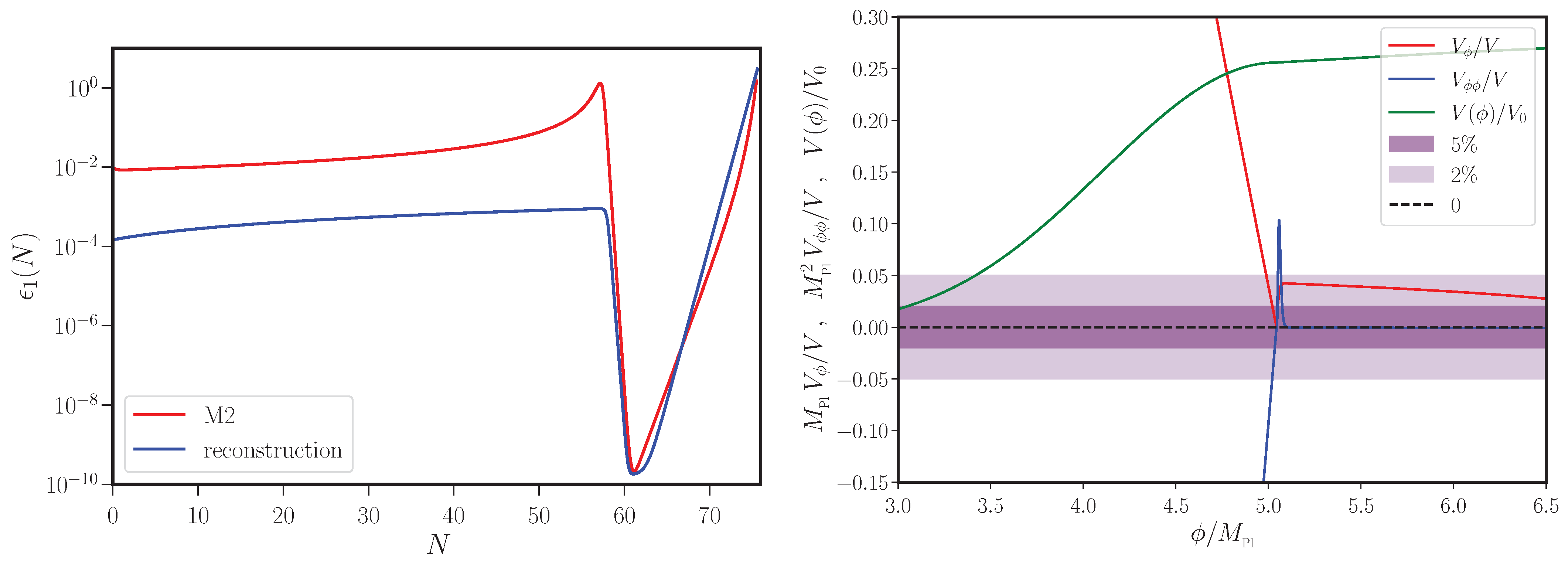
We have seen that, while the models M1 to M6 lead to an epoch of ultra slow roll inflation and to a strong peak in the scalar power spectrum on small scales, they generate primordial spectra that are not consistent with the CMB data on large scales. Actually, the hurdle seems to crop up in most single field models involving the canonical scalar field wherein ultra slow roll inflation is achieved with the aid of a (near) inflection point in the potential. When one attempts to modify the parameters so that the spectra are consistent with the CMB data, two challenges are encountered. Either there arises a prolonged duration of inflation or the power at small scales is not enhanced significantly. Moreover, in such models, it proves to be difficult to shift the location of the peak in the power spectrum. In particular, when the peak is higher and is closer the CMB scales, the inconsistency with the CMB data turns out to be greater.
A method to overcome these difficulties in canonical, single field models of inflation is to reverse engineer potentials that simultaneously lead to spectra that are consistent with the constraints from the CMB on large scales and produce significant power on small scales (for discussions in this context, see Refs. [49,53,59,120,121]). In order to do so, one begins with the desired functional form of the first slow roll parameter ϵ 1 ( N ) , i.e., one that admits a brief period of ultra slow roll after an initial epoch of slow roll, before the termination of inflation. Given ϵ 1 ( N ) , from the definition (9) of the first slow roll parameter, we can express the time evolution of the scalar field ϕ ( N ) and the Hubble parameter H ( N ) in terms of the following integrals:
        ϕ ( N ) = ϕ i M Pl N i N d N 2 ϵ 1 ( N ) ,
H ( N ) = H i exp N i N d N ϵ 1 ( N ) ,
where ϕ i and H i are the values of the scalar field and the Hubble parameter specified at some initial e-fold N i . In other words, if the initial conditions ϕ i and H i are provided, the functional form of ϵ 1 ( N ) completely determines ϕ ( N ) and H ( N ) . It is easy to show that, using the Friedmann Equation (6) and the definition of the first slow roll parameter, the potential V ( N ) can be expressed in terms of H ( N ) and ϵ 1 ( N ) as
V ( N ) = M Pl 2 H 2 ( N ) 3 ϵ 1 ( N ) .
Therefore, using ϵ 1 ( N ) and H ( N ) , we can construct V ( N ) as well. Also, as should be clear from the above equation, we require H i to determine the overall amplitude of the potential. With ϕ ( N ) and V ( N ) at hand, we can then construct the potential V ( ϕ ) parametrically. We should add that, once we have ϕ ( N ) and H ( N ) , all the other background quantities can be computed using them.
We shall consider the following form for ϵ 1 ( N ) which leads to an intermediate epoch of ultra slow roll inflation for suitable choice of the parameters involved [49]:
ϵ 1 ( N ) = ϵ 1 a 1 + ϵ 2 a N 1 tanh N N 1 Δ N 1 + ϵ 1 b + exp N N 2 Δ N 2 .
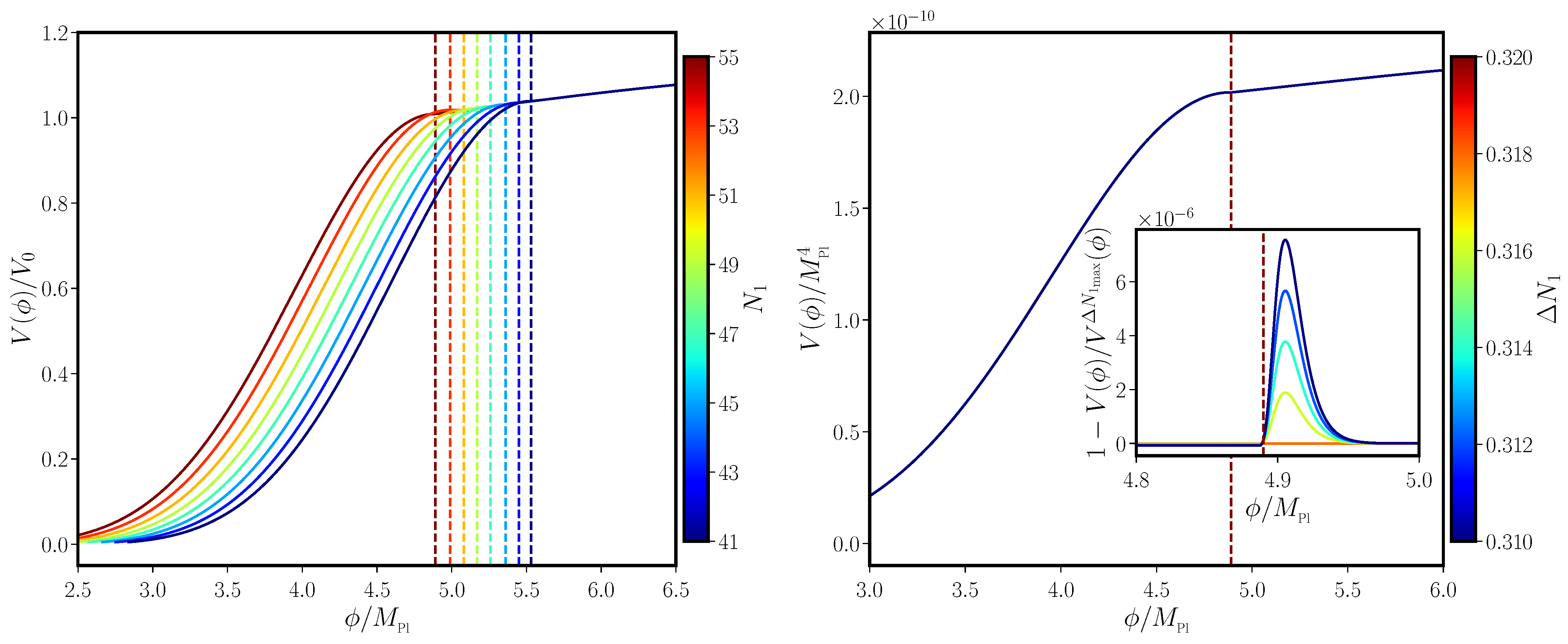
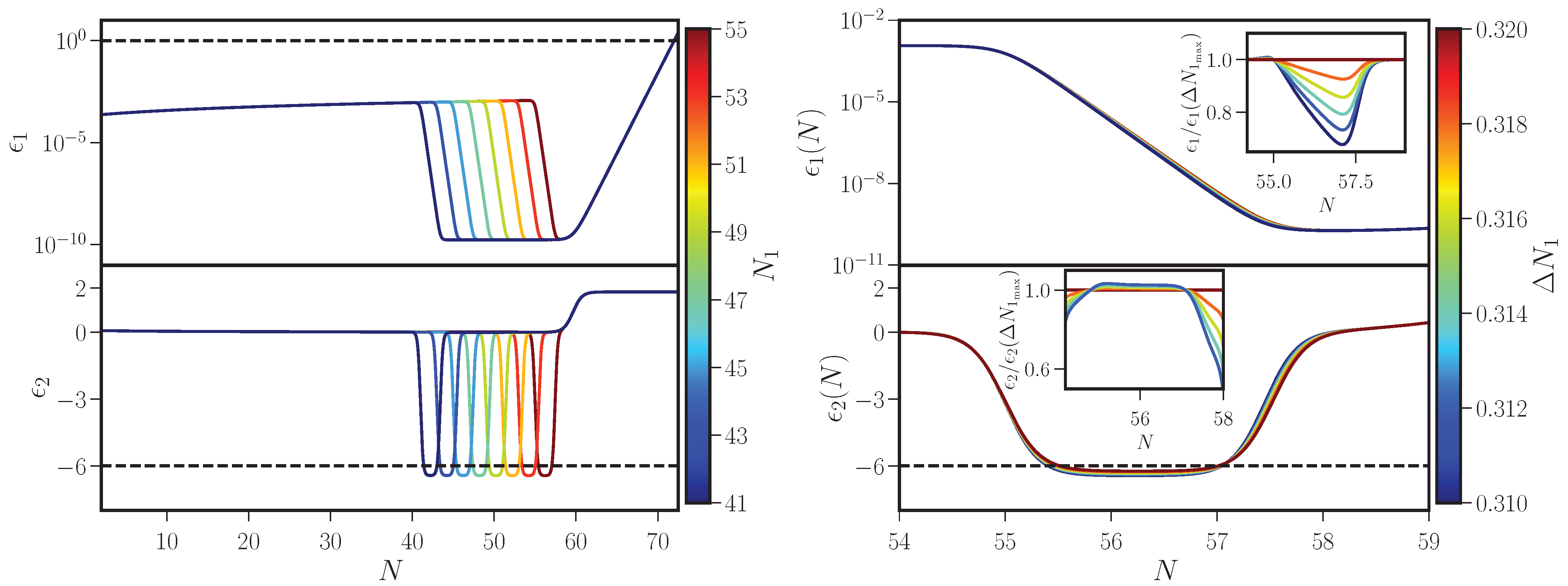
Given such a form for ϵ 1 , apart from arriving at the potential describing the background, we can determine the coefficients in Equation (28) and evolve the perturbations from the initial conditions (30) to eventually arrive at the scalar and tensor power spectra. Let us clarify a few points regarding the parameters ( ϵ 1 a , ϵ 2 a , N 1 , Δ N 1 , ϵ 1 b , N 2 , Δ N 2 ) that appear in the above expression for ϵ 1 ( N ) . The first term within the square brackets containing the parameters ϵ 1 a and ϵ 2 a leads to an initial epoch of slow roll inflation. We can choose these two parameters suitably so that the resulting scalar and tensor power are consistent with the CMB data on large scales. The hyperbolic tangent function in the first term helps us achieve the epoch of ultra slow roll, which sets in at N 1 when counted from an initial e-fold N i and the transition from slow roll to ultra slow roll inflation occurs over a duration Δ N 1 . The parameter ϵ 1 b corresponds to the value of the first slow roll parameter at the end of the regime of ultra slow roll. The exponential function in the last term leads to a rise in the first slow parameter leading to an end of inflation. Inflation ends at the e-fold N 2 and the parameter Δ N 2 regulates the duration between the end of ultra slow roll and the termination of inflation. Apart from the values of these parameters, we need to provide the initial value of H i which influences the overall amplitude of the potential and hence the power spectra. We work with the following values of the parameters involved: H i = 8.5 × 10 6 M Pl , ϵ 1 a = 7.38 × 10 5 , ϵ 2 a = 9 × 10 2 , ϵ 1 b = 1.7 × 10 10 , N 2 = 72 and Δ N 2 = 5.5 × 10 1 . We vary N 1 and Δ N 1 over the ranges [ 41 , 55 ] and [ 0.31 , 0.32 ] , respectively, to illustrate their effects on the background quantities and hence on the observables.
In Figure 4 and Figure 5, we have plotted the evolution of the first two slow roll parameters and the resulting scalar and tensor power spectra. In fact, we have plotted these quantities over the range of N 1 and Δ N 1 that we mentioned above. Note that the first two slow roll parameters broadly behave in the same manner as they did in the case of the models M1 to M6. For the values of the parameters we have worked with, the amplitude of the scalar power spectrum at the pivot scale of k * = 0.05 Mpc 1 proves to be A S = 2.10 × 10 9 . Also, we find that the scalar spectral index and the tensor-to-scalar ratio are given by n S = 0.968 and r = 1.18 × 10 3 , which are consistent with the CMB data. It is the additional parameters that are available in the parametrization of ϵ 1 ( N ) which permit us to arrive at spectra that are consistent with the CMB observations. We should also point out that, surprisingly, in complete contrast to the scalar power spectrum, the tensor power spectrum is nearly scale invariant and does not contain any feature at all.

3. Formation of PBHs in the Radiation Dominated Epoch

In this section, we shall discuss the extent of PBHs that are formed due to the enhanced power in the scalar spectra on small scales. Specifically, we shall be interested in calculating the function f PBH ( M ) , which describes the fractional contribution of PBHs to the dimensionless parameter Ω c that describes the density of cold matter today, as a function of the mass M of the PBHs.
Recall that scales with wave numbers k 10 2 Mpc 1 renter the Hubble radius during the radiation dominated epoch. Once these scales are inside the Hubble radius, the perturbations in the matter density at the corresponding scales collapse to form structures. Let the density contrast in matter be characterized by the quantity δ . The matter power spectrum P δ ( k ) during the radiation dominated epoch is related to the scalar power spectrum P S ( k ) generated during inflation though the relation [79]
P δ ( k ) = 16 81 k a H 4 P S ( k ) .
As we shall see, the fraction of PBHs formed when matter collapses after the modes reenter the Hubble radius is determined by the quantity σ 2 ( R ) , which represents the variance in the spatial density fluctuations that has been smoothed over a length scale R. The variance σ 2 ( R ) smoothed with the aid of the window function W ( k R ) is defined as [79]
σ 2 ( R ) = 0 d k k P δ ( k ) W 2 ( k R ) .
In our discussion below, we shall work with the following Gaussian form for the window function: W ( k R ) = exp [ ( k 2 R 2 ) / 2 ] .
As we mentioned, our aim will be to arrive at the number of PBHs formed as a function of their mass. To do so, we need to relate the mass M of the PBHs to the smoothing scale R that we have introduced through the window function. If M H represents the mass within the Hubble radius H 1 at a given time, it seems reasonable to assume that a certain fraction of the total mass goes on to form PBHs. Let the parameter γ reflect the efficiency of the collapse of the density contrast to form PBHs. In such a case, when a scale with wave number k reenters the Hubble radius, we can express the mass of the PBHs formed to be M = γ M H . Since no other scale is present, it seems reasonable to set k = R 1 and use the fact that k = a H when the perturbation with wave number k reenters the Hubble radius, to obtain the relation between R and M. It can be easily shown that R and M are related as follows:
R = 2 1 / 4 γ 1 / 2 g * , k g * , eq 1 / 12 1 k eq M M eq 1 / 2 ,
where k eq denotes the wave number that reenters the Hubble radius at the time of radiation-matter equality, and the quantity M eq represents the mass within the Hubble radius at equality. Moreover, the quantities g * , k and g * , eq denote the effective number of relativistic degrees of freedom at the times of PBH formation and radiation-matter equality, respectively. One finds that M eq = 5.83 × 10 47 kg and using this result, the above relation between R and M can be expressed in terms of the solar mass M as follows:
R = 4.72 × 10 7 γ 0.2 1 / 2 g * , k g * , eq 1 / 12 M M 1 / 2 Mpc .
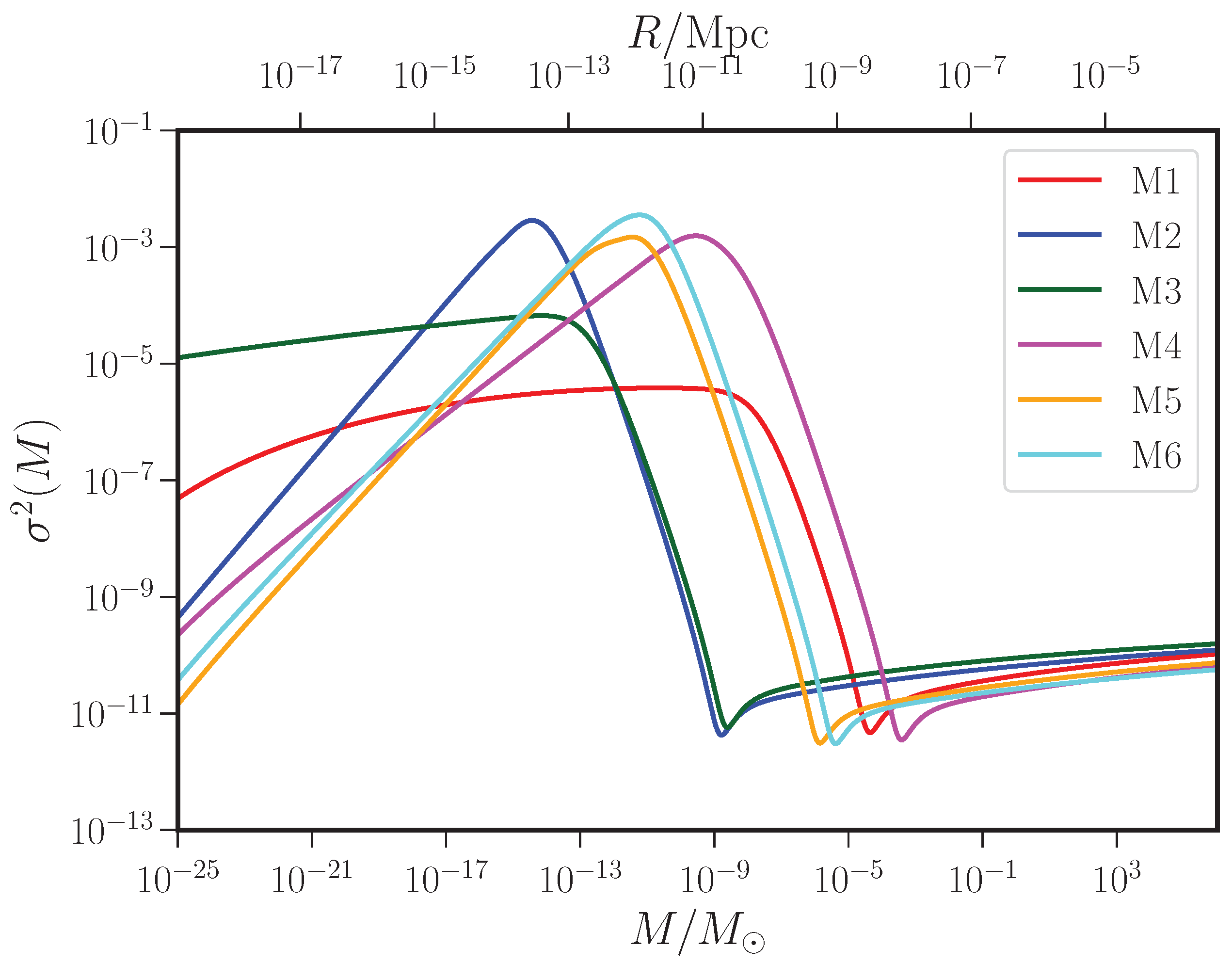
Given an inflationary scalar power spectrum P S ( k ) , we can make use of the relations (34), (35) and (37) to compute the quantity σ 2 ( M ) . In Figure 6, we have illustrated the variance σ 2 ( M ) corresponding to the scalar power spectra that arise in the inflationary models M1 to M6. As can be expected, the variance exhibits peaks over smoothing scales corresponding to the wave numbers containing the peaks in the scalar power spectra, i.e., at R k 1 (cf. Figure 3).
To calculate the number of PBHs produced, we shall assume that the density contrast δ is a Gaussian random variable described by the probability density
P M ( δ ) = 1 2 π σ 2 ( M ) exp δ 2 2 σ 2 ( M ) .
The quantity σ 2 ( M ) in this expression is the variance of the density fluctuations smoothed over the scale R that we introduced above, with R and M being related by Equation (37). Let us further assume that perturbations with a density contrast beyond a certain threshold, say, δ c , go on to form PBHs. In such a case, the fraction, say, β ( M ) , of the density fluctuations that collapse to form PBHs is described by the integral (in this context, see the reviews [29,30,31,32])
β ( M ) = δ c 1 d δ P M ( δ ) 1 2 1 erf δ c 2 σ 2 ( M ) ,
where erf ( z ) denotes the error function. We should stress here that the quantity β ( M ) is exponentially sensitive to the choice of the threshold value of the density contrast δ c , as much as it is to variance σ 2 ( M ) . Importantly, the choice of δ c is not unique and, actually, it can depend on the amplitude of the perturbation at a given scale as well as on the epoch of formation of the PBHs (for early discussions in this context, see Refs. [26,122]; for some recent discussions, see Refs. [31,89,123,124,125,126]). In our results that we present below, we shall work with δ c = 0.45 (for further details in this regard, see Refs. [127,128,129], especially Ref. [129]).
On using the arguments presented above and propagating the density of PBHs produced to the current epoch, we find that the quantity f PBH ( M ) can be written as
f PBH ( M ) = 2 1 / 4 γ 3 / 2 β ( M ) Ω m h 2 Ω c h 2 g * , k g * , eq 1 / 4 M M eq 1 / 2 ,
where Ω m and Ω c are the dimensionless parameters describing the matter and cold matter densities, with the Hubble parameter expressed as H 0 = 100 h km sec 1 Mpc 1 . In our estimates of f PBH ( M ) , we shall choose γ = 0.2 , g * , k = 106.75 and g * , eq = 3.36 . We shall also set Ω m h 2 = 0.14 and Ω c h 2 = 0.12 , which are the best fit values from the recent Planck data [130,131]. On substituting these values, we arrive at the following expression for f PBH ( M ) :
f PBH ( M ) = γ 0.2 3 / 2 β ( M ) 1.46 × 10 8 g * , k g * , eq 1 / 4 M M 1 / 2 .
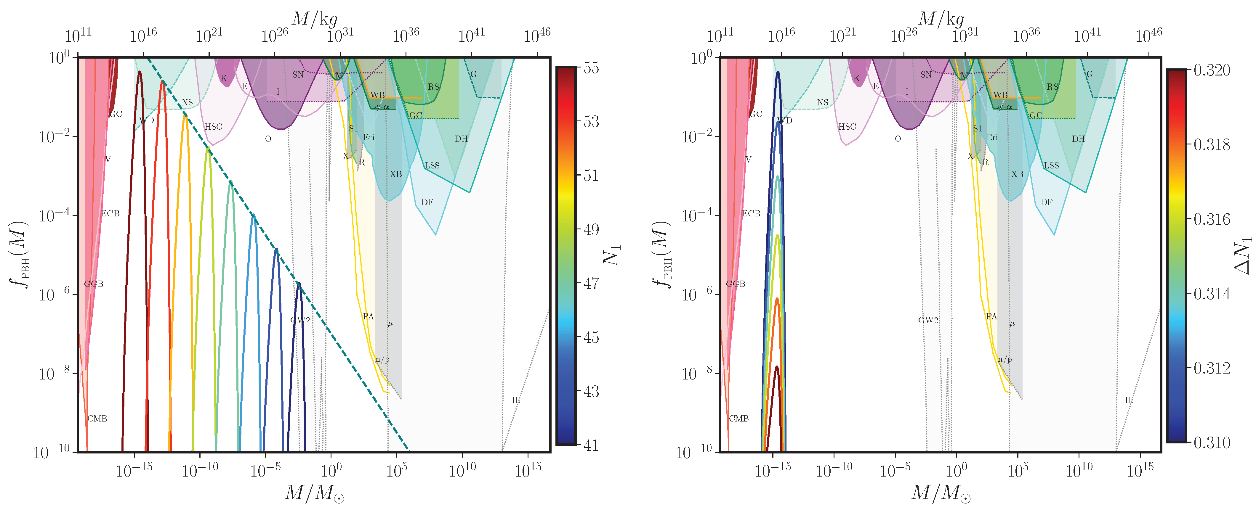
As we have discussed, given an inflationary scalar power spectrum P S ( k ) , the relations (34), (35) and (37) can be utilized to arrive at the variance σ 2 ( M ) . Once we have obtained σ 2 ( M ) , we can evaluate the quantity β ( M ) using the expression (39). Finally, we can use the relation (41) to arrive at f PBH ( M ) . In Figure 7 and Figure 8, we have plotted the quantity f PBH ( M ) in the different inflationary models and the reconstructed scenario that we discussed in the previous section. We have also included the constraints from the different observations in the figure, which correspond to a monochromatic spectrum of PBHs (in this regard, see the discussions in Refs. [33,132,133,134] and references therein). In the case of the reconstructed scenario, we have plotted the quantity f PBH ( M ) for a range of values of N 1 and Δ N 1 . Recall that, while N 1 denotes the e-fold at which the phase of ultra slow roll sets in, Δ N 1 determines the duration of the transition from the initial slow roll phase to the ultra slow roll epoch. We find that, among the six inflationary models we have considered, it is only the inflationary models M2 and M6 that produce a significant number of PBHs. In the reconstructed scenario with varied values of N 1 , the peaks in f PBH ( M ) roughly behave as M 1 / 2 , as can be expected from the relation (41) for a constant amplitude of β ( M ) that is shifted only by the mass M. This is a direct consequence of delaying the onset of ultra slow roll to later and later stages of inflation while retaining a fixed amplitude and shape of the scalar power spectrum P S ( k ) .

4. Generation of Secondary GWs in the Radiation Dominated Epoch

In Section 2, we had discussed the evolution of the scalar and tensor perturbations during inflation. We had seen that, at the linear order in the perturbations (or, equivalently, at the quadratic order in the action), the scalar and tensor perturbations evolve independently (cf. Equations (13) and (14)), a result that is often referred to as the decomposition theorem. But, when the perturbations at the second order are taken into account, one finds that the second order scalar perturbations can source the tensor perturbations (for the original discussions in this context, see Refs. [61,62,63,64]). Such a phenomenon becomes important particularly in the scenarios involving ultra slow roll inflation that we have considered. The enhanced scalar power on small scales can source the tensor perturbations to such an extent that the strength of the induced, secondary GWs can be significantly larger than the amplitude of the primary GWs generated during inflation. In this section, our aim will be calculate the dimensionless spectral energy density of the secondary GWs, say, Ω GW , induced by the scalar perturbations in the inflationary models and reconstructed scenario of interest. Specifically, we shall focus on the situation wherein the secondary GWs are generated when the scales of interest have reentered the Hubble radius during the radiation dominated era. As we shall see, interestingly, in many situations, the spectral energy density of the secondary GWs generated in such a manner can be comparable to the sensitivity curves of some of the ongoing as well as forthcoming GW observatories (in this regard, see, for instance, Refs. [70,135,136] and references therein).
We shall first sketch the essential arguments for calculating the quantity Ω GW ( f ) , where f is the frequency associated with the wave number k that can be determined by the relation
f = k 2 π = 1.55 × 10 15 k 1 Mpc 1 Hz .
For simplicity, we shall assume that the anisotropic stresses are absent during the era of radiation domination. In such a case, the scalar perturbations at the first order can be described by the Bardeen potential, say, Φ . Recall that, earlier, we had represented the first order tensor perturbations as γ i j (cf. Equation (12)). In order to distinguish the first and the second order tensor perturbations, we shall denote the second order tensor perturbations as h i j 2. On taking into account the first order scalar and the second order tensor perturbations, the FLRW line-element can be written as
d s 2 = a 2 ( η ) 1 + 2 Φ d η 2 + 1 2 Φ δ i j + 1 2 h i j d x i d x j .
Let h k denote the Fourier modes associated with the second order tensor perturbations. In terms of the mode functions h k , the tensor perturbations h i j can be decomposed as follows:
h i j ( η , x ) = d 3 k ( 2 π ) 3 / 2 e i j + ( k ) h k + ( η ) + e i j × ( k ) h k × ( η ) e i k · x ,
where quantities e i j + ( k ) and e i j × ( k ) denote the polarization tensors. As in the case of the first order tensor perturbations γ i j , the second order tensor perturbations h i j too are transverse and traceless, i.e., they satisfy the conditions δ i j k i e j l λ = δ i j e i j λ = 0 . The transverse nature of the tensor perturbations implies that the polarization tensors have non-zero components only in the plane perpendicular to the direction of propagation k ^ . The polarization tensors e i j + ( k ) and e i j × ( k ) can be expressed in terms of the set of orthonormal unit vectors ( e ( k ) , e ¯ ( k ) , k ^ ) in the following manner (for a discussion on this point, see, for example, the review [137]):
e i j + ( k ) = 1 2 e i ( k ) e j ( k ) e ¯ i ( k ) e ¯ j ( k ) ,
e i j × ( k ) = 1 2 e i ( k ) e ¯ j ( k ) + e ¯ i ( k ) e j ( k ) .
The orthonormal nature of the vectors e ( k ) and e ¯ ( k ) lead to the normalization condition: δ i l δ j m e i j λ ( k ) e l m λ ( k ) = δ λ λ , where λ and λ can represent either of the two states of polarization + or ×.
Let us now turn our attention to the equation of motion governing the modes functions h k . The equation of motion can be arrived at using the second order Einstein equations describing the tensor perturbations h i j and the Bardeen equation describing the scalar perturbation Φ at the first order (for the initial discussions, see Refs. [61,62]; for some of the recent discussions, see Refs. [66,138,139,140]). It can be shown that, during the radiation dominated epoch, the equation governing h k can be written as
h k λ + 2 η h k λ + k 2 h k λ = S k λ ,
where the quantity S k λ denotes the source due to the scalar perturbations. The source term S k λ is given by
S k λ ( η ) = 4 d 3 p ( 2 π ) 3 / 2 e λ ( k , p ) { 2 Φ p ( η ) Φ k p ( η ) + Φ p ( η ) + η Φ p ( η ) Φ k p ( η ) + η Φ k p ( η ) } ,
where Φ k represents the Fourier modes associated with the Bardeen potential and, for convenience, we have defined the quantity e λ ( k , p ) = e i j λ ( k ) p i p j . As is well known, during the epoch of radiation domination, we can express the Fourier modes Φ k of the Bardeen potential in terms of the Fourier modes R k of the curvature perturbations generated during inflation through the relation
Φ k ( η ) = 2 3 T ( k η ) R k ,
where T ( k η ) is the transfer function given by
T ( k η ) = 9 k η 2 sin k η / 3 k η / 3 cos k η / 3 .
If we make use of the Green’s function corresponding to the tensor modes during radiation domination, we find that we can express the inhomogeneous contribution to h k λ as [66]
h k λ ( η ) = 4 9 k 3 η d 3 p ( 2 π ) 3 / 2 e λ ( k , p ) R k R k p × I c p k , | k p | k cos k η + I s p k , | k p | k sin k η ,
where the quantities I c ( v , u ) and I s ( v , u ) are described by the integrals
I c ( v , u ) = 4 0 d τ τ sin τ { 2 T ( v τ ) T ( u τ ) + T ( v τ ) + v τ T v τ ( v τ ) T ( u τ ) + u τ T u τ ( u τ ) } ,
I s ( v , u ) = 4 0 d τ τ cos τ { 2 T ( v τ ) T ( u τ ) + T ( v τ ) + v τ T v τ ( v τ ) T ( u τ ) + u τ T u τ ( u τ ) } ,
with T z = d T / d z . Upon utilizing the transfer function (49), these integrals can be calculated analytically to obtain that (see, for example, Refs. [65,66])
I c ( v , u ) = 27 π 4 v 3 u 3 Θ v + u 3 ( v 2 + u 2 3 ) 2 ,                                                                                                            
I s ( v , u ) = 27 4 v 3 u 3 ( v 2 + u 2 3 ) 4 v u + ( v 2 + u 2 3 ) log 3 ( v u ) 2 3 ( v + u ) 2 ,
where Θ ( z ) denotes the theta function. It is useful to note that I c , s ( v , u ) = I c , s ( u , v ) .
The power spectrum of the secondary GWs, say, P h ( k , η ) , generated due to the second order scalar perturbations can be defined through the relation
h k λ ( η ) h k λ ( η ) = 2 π 2 k 3 P h ( k , η ) δ ( 3 ) ( k + k ) δ λ λ .
It should be evident that, because the quantity h k λ involves products of the Fourier modes R k and R k p of the curvature perturbations generated during inflation (see Equation (50)), the power spectrum P h ( k ) of the secondary GWs will involve products of four such variables. If we assume that the Fourier modes of the curvature perturbations are Gaussian random variables, we can express the four-point function involving R k in terms of the two-point functions, i.e., in terms of the the inflationary scalar power spectrum P S ( k ) (cf. Equation (18a)). Equivalently, it can be said that, since the expectation value in the definition (53) of the secondary tensor power spectrum has to be evaluated in the Bunch-Davies vacuum, the four-point function of the curvature perturbations can be expressed in terms of the two-point functions using Wick’s theorem. Upon doing so, we can arrive at the following expression for the secondary tensor power spectrum:
P h ( k , η ) = 4 81 k 2 η 2 0 d v | 1 v | 1 + v d u 4 v 2 ( 1 + v 2 u 2 ) 2 4 u v 2 P S ( k v ) P S ( k u ) × I c ( u , v ) cos k η + I s ( u , v ) sin k η 2 .
The trigonometric functions in this expression arise because of the form of the transfer function T ( k η ) (cf. Equation (49)). They reflect the fact that the Bardeen potentials Φ k oscillate when the corresponding scales are inside the Hubble radius during the radiation dominated epoch. On averaging the secondary tensor power P h ( k , η ) over small time scales, we can replace the trigonometric functions in the above expression by their average over a time period. In such a case, only the overall time dependence remains, leading to [65,66]
P h ( k , η ) ¯ = 2 81 k 2 η 2 0 d v | 1 v | 1 + v d u 4 v 2 ( 1 + v 2 u 2 ) 2 4 u v 2 P S ( k v ) P S ( k u ) × I c 2 ( u , v ) + I s 2 ( u , v ) ,
where the line over P h ( k , η ) implies that we have averaged over small time scales. The energy density of GWs associated with a Fourier mode corresponding to the wave number k (i.e., the spectral energy density of GWs) at a time η is given by [137]
ρ GW ( k , η ) = M Pl 2 8 k a 2 P h ( k , η ) ¯ .
We can define the corresponding dimensionless density parameter Ω GW ( k , η ) in terms of the critical density ρ cr ( η ) as [66]
Ω GW ( k , η ) = ρ GW ( k , η ) ρ cr ( η ) = 1 24 k H 2 P h ( k , η ) ¯ = k 2 η 2 24 P h ( k , η ) ¯ ,
where, in the final expression, we have made use of the fact that H = 1 / η in radiation domination era. Note that, since P h ( k , η ) η 2 , the dimensionless spectral energy density Ω GW ( k , η ) is actually independent of time.
The dimensionless spectral density of GWs above has been calculated during the late stages of the epoch of radiation domination, when all the scales of interest are inside the Hubble radius. In such a domain, the energy density of GWs decreases in the same fashion as the energy density of radiation (i.e., as a 4 ). Utilizing this behavior, we can express the dimensionless spectral energy density of GWs today, i.e., Ω GW ( k ) , in terms of the Ω GW ( k , η ) above in the following manner
h 2 Ω GW ( k ) = g * , k g * , 0 1 / 3 Ω r h 2 Ω GW ( k , η ) 1.38 × 10 5 g * , k 106.75 1 / 3 Ω r h 2 4.16 × 10 5 Ω GW ( k , η ) .
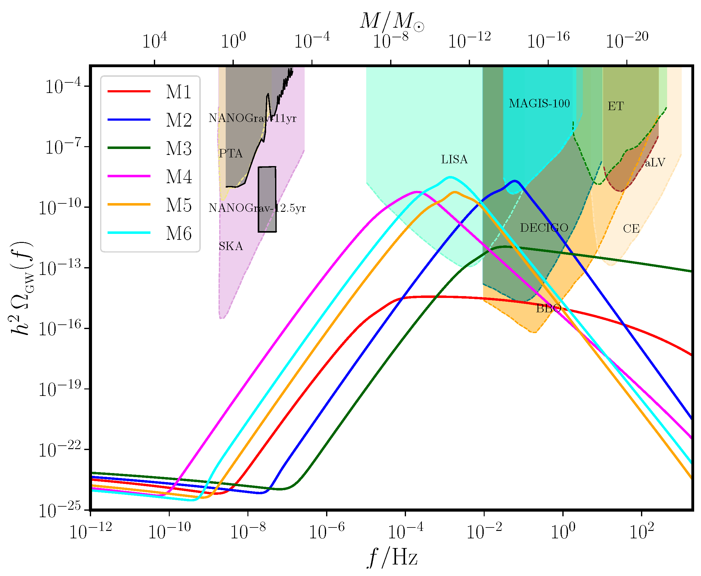
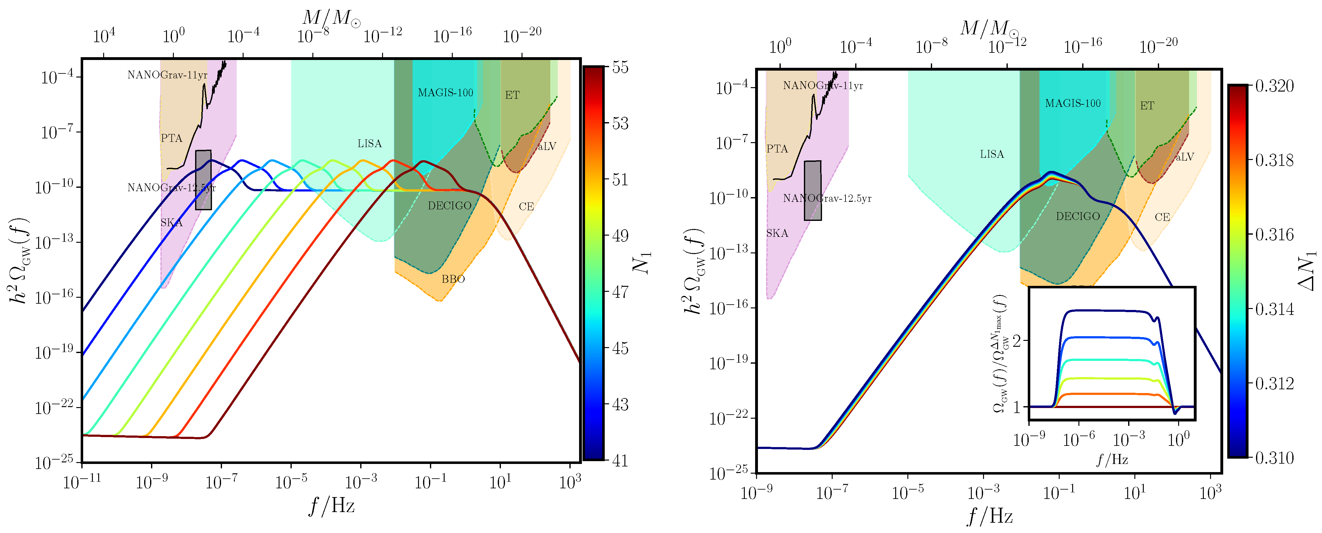
In this expression, Ω r and g * , 0 denote the dimensionless energy density of radiation and the number of relativistic degrees of freedom today. In Figure 9 and Figure 10, we have plotted the quantity Ω GW as a function of the frequency f in the six inflationary models and the reconstructed scenario we have considered. We have also included the sensitivity curves of the different ongoing as well as forthcoming GW observatories in the figures (in this context, see, for example, Refs. [70,135,136,141,142]). It is clear that all the models and the reconstructed scenario lead to GW spectral densities that are comparable to the sensitivity curves of the different observatories. This gives us hope that the imprints of non-trivial dynamics during the late stages of inflation can either be detected or, at the least, strongly constrained with the aid of GW observations set to emerge over the coming decade or two.

5. Non-Gaussianities on Small Scales

As we have seen, the onset of ultra slow roll leads to strong departures from slow roll inflation with the second slow roll parameter ϵ 2 (as well as the higher order slow roll parameters) attaining rather large values. It is the strong departure from slow roll that results in sharp features in the scalar power spectrum, such as the peak with significantly enhanced power that we have discussed earlier. We should clarify that, we have chosen the parameters of the inflationary potentials and the reconstructed scenario so that the ultra slow roll phase sets in during the latter stages of inflation (after the wave numbers corresponding to the CMB scales have left the Hubble radius) and the peak occurs at small scales.
In fact, there has been a constant effort in the literature to investigate if certain features in the inflationary scalar power spectrum provide a better fit to the CMB data than the more standard, nearly scale invariant spectrum (see the recent efforts [78,145,146] and references therein). Often, these features are generated due to moderate departures from slow roll inflation. However, we should point out that strong departures such as those occur in ultra slow roll inflation have been considered to suppress the power on the largest scales (comparable to the Hubble radius today) so as to improve the fit to the lowest multipoles in the CMB data [78,110,111]. In slow roll inflation involving the canonical scalar field, typically, the non-Gaussianities generated are rather small with the dimensionless parameter f NL  (defined below in Equation (67)) that reflects the amplitude of the scalar bispectrum being of the order of the first slow roll parameter ϵ 1 [71,72,73,77,78]. But, when departures from slow roll occur, it is known that the amplitude of the scalar bispectrum and the associated non-Gaussianity parameter can be considerably larger [73,77,78]. Moreover, while the scalar bispectrum has an equilateral shape in slow roll inflation, the shape can be considerably different when deviations from slow roll occur. These suggest that the epoch of ultra slow roll inflation that we have considered to enhance power on small scales can also be expected to generate significant levels of non-Gaussianities with characteristic shapes [78].
In this section, we shall compute the scalar bispectrum and the associated non-Gaussianity parameter for two of the inflationary models that we have discussed earlier. However, before we go on to present these results, we shall first describe the third order action that governs the curvature perturbations and the numerical method we shall adopt to compute the scalar bispectrum.

5.1. The Complete Third Order Action Governing the Scalar Bispectrum

Let us begin by recalling a few necessary points regarding the scalar bispectrum. Just as the power spectrum characterizes the two-point function of the perturbations in Fourier space, the bispectrum describes corresponding three-point function. The scalar bispectrum, say, B S ( k 1 , k 2 , k 3 ) , is defined in terms of the operator R ^ k (that we had introduced earlier in Equation (15a)) as follows [14,15]:
R ^ k 1 ( η e ) R ^ k 2 ( η e ) R ^ k 3 ( η e ) = ( 2 π ) 3 B S ( k 1 , k 2 , k 3 ) δ ( 3 ) ( k 1 + k 2 + k 3 ) ,
where η e is a time close to the end of inflation and the expectation value on the left hand side is to be evaluated in the perturbative vacuum [71,72,75]. Note that the delta function that appears in the above definition implies that the three wave vectors ( k 1 , k 2 , k 3 ) form the edges of a triangle. Hence, it is only two of the vectors that are truly independent and, it is for this reason the quantity B S ( k 1 , k 2 , k 3 ) is referred to as the bi-spectrum. Hereafter, for convenience, we shall set
B S ( k 1 , k 2 , k 3 ) = ( 2 π ) 9 / 2 G ( k 1 , k 2 , k 3 )
and refer to G ( k 1 , k 2 , k 3 ) as the scalar bispectrum.
Conventionally, in quantum field theory, the correlation functions beyond the two-point functions that describe the fields are often calculated using perturbative methods. As is well known, the three-point function associated with a field can be expected to be non-zero if the action governing the field of interest contains a cubic order term. The same approach can be utilized to calculate the scalar bispectrum generated during inflation (for the original discussions in this context, see Refs. [71,72,73]). Evidently, in order to do so, one first requires the action describing the curvature perturbation at the third order. With such an action at hand, one can use the standard methods of perturbative quantum field theory to arrive at the scalar bispectrum.
Recall that, in Section 2, we had arrived at the action and the equations of motion governing the background as well as the scalar and tensor perturbations using the ADM formalism. Starting from the original action (2) that governs the system of the gravitational and scalar fields and the line-element (12), the third order action describing the curvature perturbation can arrived at in the same manner [71,72,73,76]. In fact, a set of temporal and spatial boundary terms arise in the process, when the action is repeatedly integrated by parts to simplify its form. One can easily establish that, due to the triangularity condition on the wave vectors ( k 1 , k 2 , k 3 ) , the spatial boundary terms do not contribute to the scalar bispectrum under any condition. However, some of the temporal boundary terms can contribute to the scalar bispectrum even in the simple case of slow roll inflation [102]. It can be shown that, at the third order, the action governing the curvature perturbation R can be expressed as (see, for instance, Refs. [71,72,76,102])
S 3 [ R ] = M Pl 2 d η d 3 x [ a 2 ϵ 1 2 R R 2 + a 2 ϵ 1 2 R ( R ) 2 2 a ϵ 1 R ( R ) ( χ ) + a 2 2 ϵ 1 ϵ 2 R 2 R + ϵ 1 2 ( R ) ( χ ) 2 χ + ϵ 1 4 2 R ( χ ) 2 + 2 F ( R ) δ L 2 δ R ] ,
where ϵ 1 and ϵ 2 are the slow roll parameters we have repeatedly encountered, while 2 χ = a ϵ 1 R . Moreover, the quantity F ( R ) is given by
F ( R ) = ϵ 2 4 R 2 + 1 a H R R + 1 4 a 2 H 2 ( R ) ( R ) + 2 [ i j ( i R j R ) ] + 1 2 a 2 H ( R ) ( χ ) 2 [ i j ( i R j χ ) ]
and L 2 denotes the Lagrangian density associated with the action (13a) that governs the curvature perturbation at the second order. Further, the temporal boundary terms are given by [102]
S 3 B [ R ] = M Pl 2 d η d 3 x d d η { 9 a 3 H R 3 + a H ( 1 ϵ 1 ) R ( R ) 2 1 4 a H 3 ( R ) 2 2 R a ϵ 1 H R R 2 a ϵ 2 2 R 2 2 χ + 1 2 a H 2 R i j R i j χ 2 R 2 χ 1 2 a H R i j χ i j χ ( 2 χ ) 2 } .
In most of the situations of interest, including the scenarios that we are considering here, one finds that it is only the term involving ϵ 2 (in the above expression) that contributes to the scalar bispectrum. Usually, the contribution due to this term is taken into account through a field redefinition (for a discussion in this context, see, for instance, Refs. [71,102]). Instead, apart from the calculating the contributions to the bispectrum due to the bulk terms in the action (61), we shall explicitly evaluate contribution due to the term containing ϵ 2 in Equation (63).

5.2. Numerical Computation of the Scalar Bispectrum and the Associated Non-Gaussianity Parameter

Upon taking into account the contributions due to the bulk and the boundary terms we discussed above, it can be shown that the scalar bispectrum, evaluated at a time η e close to the end of inflation, can be written as (in this context, see, for instance, Refs. [49,76,77,78])
G ( k 1 , k 2 , k 3 ) = M Pl 2 C = 1 6 f k 1 ( η e ) f k 2 ( η e ) f k 3 ( η e ) G C ( k 1 , k 2 , k 3 ) + complex conjugate + G 7 ( k 1 , k 2 , k 3 ) ,
where f k are the mode functions associated with the curvature perturbation (cf. Equation (15a)). The quantities G C ( k 1 , k 2 , k 3 ) that appear in the above expression represent six integrals that involve the scale factor, the slow roll parameters, the mode functions f k and their time derivatives f k . They correspond to the six bulk terms appearing in the cubic order action (61) and are described by the following expressions:
G 1 ( k 1 , k 2 , k 3 ) = 2 i η i η e d η a 2 ϵ 1 2 f k 1 * f k 2 * f k 3 * + two permutations ,                                                      
G 2 ( k 1 , k 2 , k 3 ) = 2 i k 1 · k 2 + two permutations η i η e d η a 2 ϵ 1 2 f k 1 * f k 2 * f k 3 * ,                          
G 3 ( k 1 , k 2 , k 3 ) = 2 i η i η e d η a 2 ϵ 1 2 k 1 · k 2 k 2 2 f k 1 * f k 2 * f k 3 * + five permutations ,                      
G 4 ( k 1 , k 2 , k 3 ) = i η i η e d η a 2 ϵ 1 ϵ 2 f k 1 * f k 2 * f k 3 * + two permutations ,                                                      
G 5 ( k 1 , k 2 , k 3 ) = i 2 η i η e d η a 2 ϵ 1 3 k 1 · k 2 k 2 2 f k 1 * f k 2 * f k 3 * + five permutations ,                            
G 6 ( k 1 , k 2 , k 3 ) = i 2 η i η e d η a 2 ϵ 1 3 k 1 2 k 2 · k 3 k 2 2 k 3 2 f k 1 * f k 2 * f k 3 * + two permutations .
These integrals are to be calculated from an early time ( η i ) when the scales of interest are well inside the Hubble radius, until a time towards the end of inflation ( η e ). We should also clarify that the last term in the action (61) involving F ( R ) ( δ L 2 / δ R ) actually vanishes when we assume that the curvature perturbation satisfies the linear equation of motion (cf. Equation (14a)). The contribution G 7 ( k 1 , k 2 , k 3 ) is due to the term containing ϵ 2 in the boundary terms (63), and it can be expressed as
G 7 ( k 1 , k 2 , k 3 ) = i M Pl 2 ( f k 1 ( η e ) f k 2 ( η e ) f k 3 ( η e ) ) × a 2 ϵ 1 ϵ 2 f k 1 * ( η ) f k 2 * ( η ) f k 3 * ( η ) + two permutations η i η e + complex conjugate .
When one imposes the initial conditions when the scales are well inside the Hubble radius, the contribution due to η i in the above expression for G 7 ( k 1 , k 2 , k 3 ) vanishes with the introduction of a regulator, and it is only the term evaluated towards end of inflation (i.e., at η e ) that contributes. Usually, instead of the scalar bispectrum, it is the dimensionless non-Gaussianity parameter f NL ( k 1 , k 2 , k 3 ) that is often quoted and constrained. The non-Gaussianity parameter corresponding to the scalar bispectrum G ( k 1 , k 2 , k 3 ) is defined as (see, for instance, Refs. [76,77])
f NL ( k 1 , k 2 , k 3 ) = 10 3 1 2 π 4 k 1 3 k 2 3 k 3 3 G ( k 1 , k 2 , k 3 ) × k 1 3 P S ( k 2 ) P S ( k 3 ) + two permutations 1 ,
where P S ( k ) denotes the scalar power spectrum (cf. Equation (20a)).
When departures from slow roll inflation occur, as in the case of the power spectrum, in general, it proves to be difficult to evaluate the scalar bispectrum analytically. Hence, one has to construct methods to compute the scalar bispectrum numerically [49,74,77,78]. As we pointed out, the quantities G C ( k 1 , k 2 , k 3 ) are described by integrals which involve the background quantities as well as the mode functions f k and their time derivatives f k (cf. Equation (65)). We have already discussed the numerical evaluation of the background quantities and the scalar mode functions f k . It is now a matter of utilizing them and carrying out the integrals describing the quantities G C ( k 1 , k 2 , k 3 ) . In analytical calculations, to evaluate these integrals, one assumes that η i and η e 0 . But, evidently, it is not possible to achieve these extreme limits in numerical computations. Actually, it does not seem to be necessary either. We had seen earlier that, to evaluate the scalar power spectrum, it is often adequate to evolve the mode functions f k from k 10 2 z / z until k 10 5 z / z . The reason being that, in most situations, the mode functions only oscillate in the sub-Hubble regime and their amplitudes quickly freeze once they leave the Hubble radius. Interestingly, one finds that, since the amplitudes of the mode functions freeze, the super-Hubble contributions to the bispectrum prove to be negligible [77]. However, in contrast to the power spectrum wherein we needed to focus on a single wave number, the bispectrum depends on three wave numbers. Therefore, we need to carry out the integrals from an early time when the smallest of the three wave numbers (in the range of our interest) satisfies the condition k 10 2 z / z until a late time when the largest of them satisfies the condition k 10 5 z / z . Also, in order to choose the correct perturbative vacuum, one has to regulate the integrals G C ( k 1 , k 2 , k 3 ) by imposing a cut-off in the sub-Hubble regime [72]. Often, in the integrals, one introduces a cut-off function that is democratic in wave number and is of the form exp κ ( k 1 + k 2 + k 3 ) / ( 3 z / z ) , where κ is a suitably chosen, positive definite and small quantity (for a discussion in this regard, see Refs. [74,77,78]). Numerically, such a cut-off proves to be convenient as it aids in the efficient computation of the integrals. In scenarios involving ultra slow roll inflation, we had pointed out that, due to the non-trivial evolution of the scalar mode functions f k at late times, it is safer to evaluate the power spectra at the end of inflation. For the same reason, we also evaluate the scalar bispectrum close to the end of inflation in the models and scenarios of our interest here3. Lastly, we should mention that the non-trivial boundary term G 7 ( k 1 , k 2 , k 3 ) is easier to compute as it does not involve any integral and depends only the background parameters, the mode function f k and its time derivative f k , evaluated at the end of inflation.
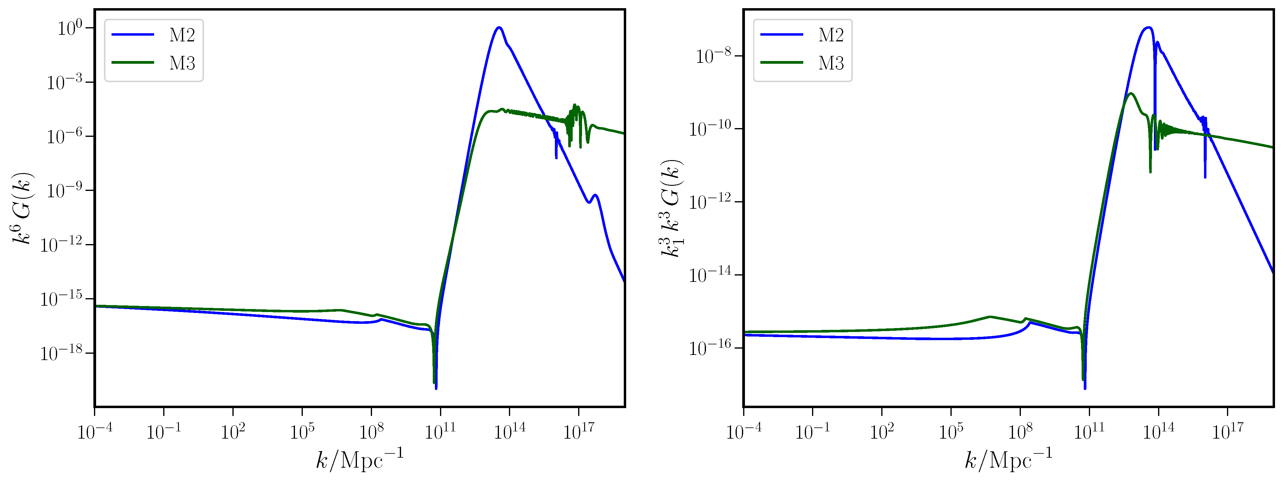
In Figure 11, we have illustrated suitable dimensionless combinations of the wave numbers ( k 1 , k 2 , k 3 ) and the bispectrum G ( k 1 , k 2 , k 3 ) in the equilateral (i.e., when k 1 = k 2 = k 3 = k ) and the squeezed limits (i.e., when k 1 0 , k 2 k 3 k ) for the inflationary models M2 (which has a narrow peak in the scalar power spectrum and M3 (which has a rather broad peak). Remarkably, the shape of the bispectra in these limits closely resemble the shape of the corresponding power spectra. However, note that, on small scales, around the peak, the amplitude of the bispectra are considerably higher in the equilateral limit than in the squeezed limit. Also, it is interesting to note that the dip and the peak in the bispectra occur at the same wave numbers as observed in the power spectra. Such a sharp dip actually implies the vanishing of the mode function f k for a specific wave number. As a result, it can be expected that any higher order correlation function involving the wave number also identically vanishes (for a detailed discussion regarding the dip, see Refs. [58,119,147,148,149]). We should add that the bispectra also contain additional features that are unique to the nature of the terms in the cubic order action and the corresponding integrals involved in the computation.
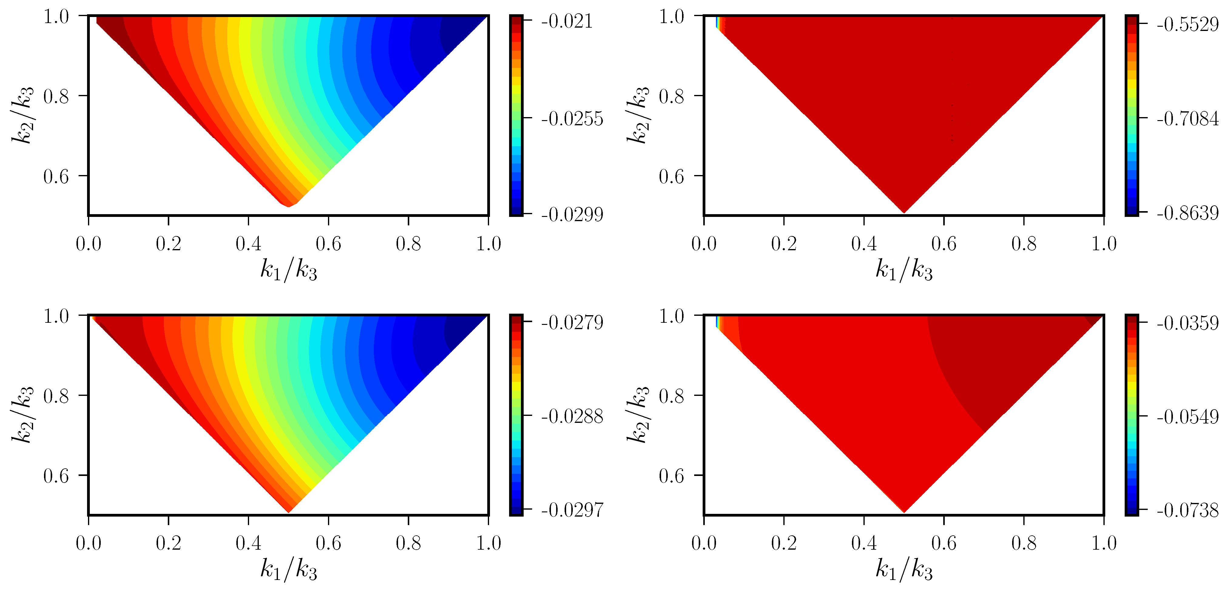
In Figure 12, we have presented the density plots of the scalar non-Gaussianity parameter f NL ( k 2 , k 2 , k 3 ) for the two inflationary models M2 and M3. We have illustrated the density of the non-Gaussianity parameter around two wave numbers chosen in two distinct regimes— k * (i.e., the pivot scale) over large scales and k peak (i.e., the wave number corresponding to the peak in the scalar power spectra) over small scales. We find that, for M2, k peak = 3.5 × 10 13 Mpc 1 and, for M3, k peak = 1.8 × 10 13 Mpc 1 . Clearly, f NL is equilateral in shape around k * with values of order O ( 10 2 ) as expected from perturbations evolving over a slow roll regime. But, the shape of f NL turns out to be local around k peak and the amplitude becomes model dependent, with values close to 0.56 for M2 and 0.05 in case of M3. An analytical understanding of the amplitude and shape of the scalar bispectrum in models permitting a brief epoch of ultra slow roll inflation is still elusive and requires attention [150]. Moreover, the behavior of bispectrum in the reconstructed scenario and the effect of the parameters such as N 1 and Δ N 1 on the associated f NL is an interesting topic of exploration. We are currently investigating these issues.

6. Outlook

In this review, we have considered ultra slow roll inflation driven by a single, canonical scalar field which leads to enhanced scalar power on small scales. We have examined the corresponding effects on the extent of formation of PBHs and the production of secondary GWs during the radiation dominated epoch. We have also computed the shape and the strengths of non-Gaussianities generated on small scales in such situations. We should mention that the numerical codes used to arrive at the results presented in this review are available at the following URL: https://gitlab.com/ragavendrahv/pbs-pbh-sgw.git 6 February 2023. The package computes the scalar and tensor power spectra as well as the scalar bispectrum for a given canonical, single field model of inflation. Further, it can compute the corresponding f PBH ( M ) and Ω GW ( f ) arising from such spectra, as discussed in this review.4
There are many related scenarios and effects that we could not include in this review. While a few of these effects have been investigated already, some of them require further study. In this concluding section, we shall describe them briefly.
  • Effects of non-Gaussianities on the formation of PBHs: In our discussion, we have restricted our attention to the effects of the increased scalar power (due to the epoch of ultra slow roll) on the number of PBHs produced. Since the amplitude of the bispectrum generated due to ultra slow roll is significantly higher than the slow roll values, the non-Gaussianities can be expected to boost the extent of PBHs formed (for earlier discussions on this point, see, for instance, Refs. [51,87,151,152]). There has been recent efforts to account for a skewness in the probability distribution describing the density contrast (cf. Equation (38)), arising due to increased strengths of the scalar bispectrum on small scales, and calculate the corresponding effects on the number of PBHs produced [90,91,92]. We should point out that alternative methods have also been proposed to account for the scalar non-Gaussianity in such calculations (see Refs. [153,154]; for a brief summary of the different methods, see Ref. [93]).
  • Effects of non-Gaussianities on secondary GWs: It has been argued that large amplitudes of f NL , as arising in ultra slow roll models, can considerably influence the strengths of secondary GWs that are generated during the radiation dominated epoch [67,95,99]. However, rather than calculate the bispectrum arising in specific inflationary models, these attempts often assume certain well motivated amplitudes and shapes of f NL to calculate the corresponding contributions to Ω GW . There have also been efforts to compute such non-Gaussian contributions to Ω GW , while accounting for complete scale dependence of f NL , arising from the bispectrum in specific models of ultra slow roll (in this regard, see Ref. [100]). These computations suggest that the non-Gaussian contributions to Ω GW are highly model dependent and can, in principle, alter the shape and amplitude of Ω GW around the peak of the spectra.
  • Loop corrections to the primordial power spectrum: There is a gathering interest in the literature towards computing the contributions due to the loops to the scalar and tensor power spectra generated during inflation (for related early efforts, see, for example Refs. [155,156,157,158]). These contributions capture the effects of the higher order correlations on the power spectra and can lead to characteristic signatures on the predicted observables. There have been attempts to investigate such effects on observables such as Ω GW and the 21-cm signals from neutral hydrogen of the Dark Ages [159,160,161]. There have also been efforts to theoretically restrict models of ultra slow roll inflation based on the amplitude of the corrections due to the loops and the associated consequences for the validity of perturbative treatment of the correlations (in this regard, see Refs. [162,163,164,165]).
We are presently investigating different issues in these directions.

Funding

H.V.R. acknowledges support from the Indian Institute of Science Education and Research Kolkata through postdoctoral fellowship. L.S. wishes to acknowledge support from the Science and Engineering Research Board, Department of Science and Technology, Government of India, through the Core Research Grant CRG/2018/002200.

Data Availability Statement

We have used data that are publicly available and we have cited the sources appropriately.

Conflicts of Interest

The authors declare no conflict of interest.

Appendix A. Determining the Locations of the Point of Inflection
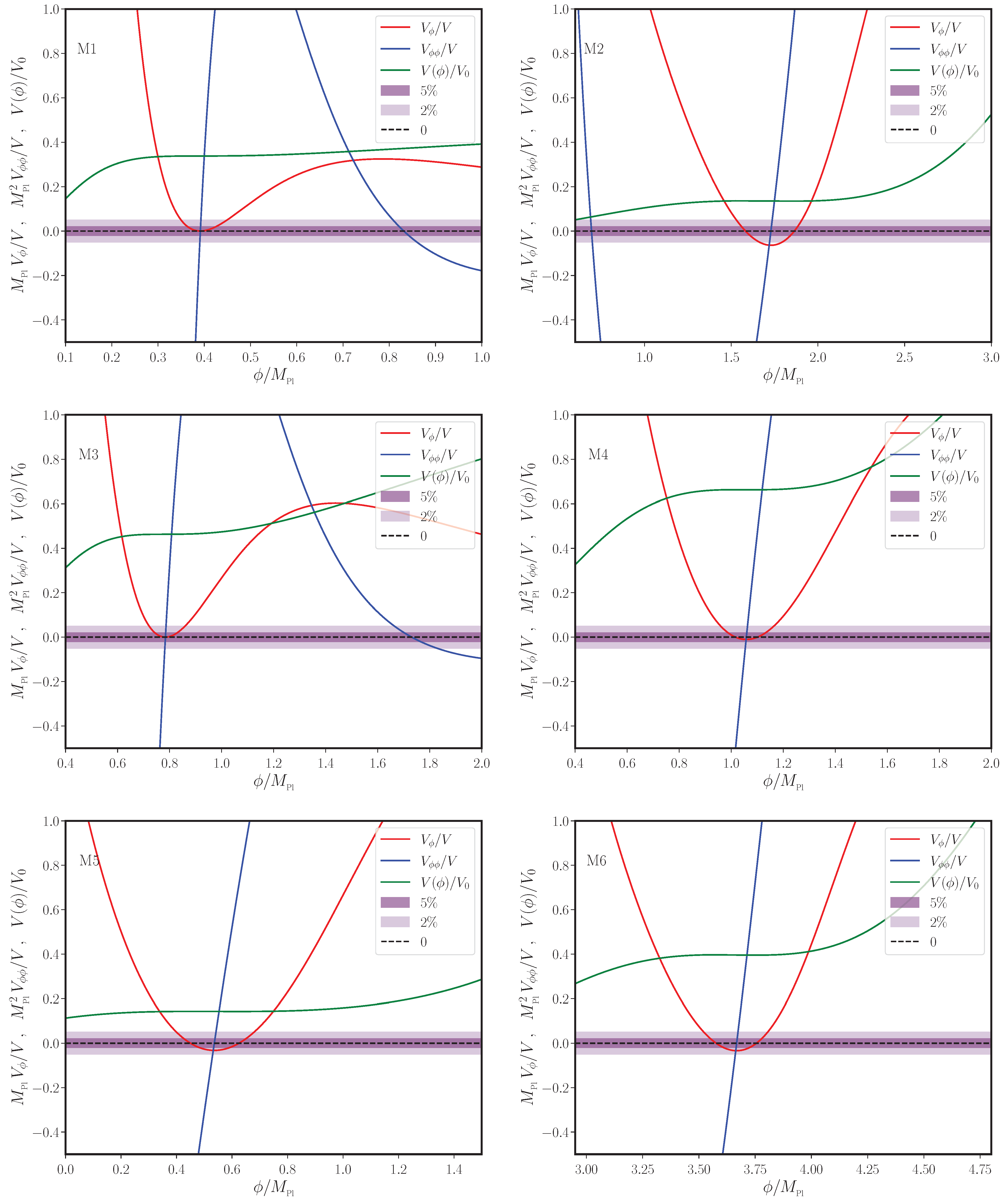
In our discussion in Section 2.2, we had mentioned the locations of the point of inflection (viz. the value of ϕ 0 ) in the inflationary models M1 to M6. We should clarify that some of these are actually near inflection points, where the first and the second derivatives of the potential V ϕ and V ϕ ϕ almost vanish. In Figure A1, we have illustrated the method by which we have identified the points of inflection. In the figure, we have plotted the behavior of the inflationary potential V as well as the quantities V ϕ / V and V ϕ ϕ / V in the six models of interest. Note that, since the first two derivatives of the potentials almost vanish at these (near) inflection points, the potentials have a plateau around the point. As the field enters the flat region of the potentials, it considerably slows down resulting in an epoch of ultra slow roll inflation in these models.
Figure A1. We have illustrated the manner in which we have numerically determined the points of inflection in the inflationary models of interest. We have plotted the quantities V ϕ / V and V ϕ ϕ / V as well as a suitably rescaled potential V in the models M1 to M6 (from the top left to the bottom right corner). In the figures, we have included bands of 2 % and 5 % around zero. The location of the point of inflection is determined by the condition that both V ϕ / V and V ϕ ϕ / V lie within 5 % of zero. While, in some of the models, these quantities lie even within 2 % of zero, we find that, in the model M2, the quantities deviate by as much as 7 % .
Galaxies 11 00034 g0a1
In Figure A2, we have plotted the potentials that correspond to the scenario described by the first slow parameter ϵ 1 ( N ) in Equation (33). As described in Section 2.5, from the form of ϵ 1 ( N ) , we have computed ϕ ( N ) and V ( N ) using Equations (31) and (32), and have plotted the potential V ( ϕ ) parametrically. We have illustrated the numerically calculated potentials for the range of N 1 and Δ N 1 discussed earlier.
Further, in Figure A3, we have presented the behavior of quantity ϵ 1 ( N ) in the reconstructed scenario (cf. Equation (33)) for a specific set of parameters that have been chosen to mimic the behavior of the first slow roll parameter in the model M2. This is to illustrate the manner in which our reconstruction captures the essential features of a typical model that permits a phase of ultra slow roll, while at the same time providing better handle on the associated dynamics. We achieve the onset and duration of the phase of ultra slow roll at e-folds similar to that of M2, and also terminate inflation around the same time as in M2. Moreover, in the reconstructed scenario, we are able to work with a lower value of ϵ 1 during the initial stage of slow roll, which ensures a viable tensor-to-scalar ratio over the CMB scales, unlike the case of M2 (cf. Table 1). In the figure, we have also illustrated the behavior of the potential (as well as its first and second derivatives) associated with the reconstructed scenario, in the same manner as we had presented for the models M1–M6 in Figure A1. We have plotted them parametrically against the field, and have focused on the behavior around the point of inflection. We notice that the point of inflection occurs quite rapidly, unlike the models M1–M6 which show a smoother behavior. The vanishing of the derivatives are rather sharp and highly coincident, in contrast to the model M2 which only contains a near-inflection point.
Figure A2. The shape of the potential obtained from reconstruction is presented for a range of values of N 1 (on the left) and Δ N 1 (on the right). Understandably, the change in N 1 moves the location of the point of inflection (marked with dashed lines of respective colors). The variation in Δ N 1 leads to imperceptibly small change in the shape of the potential around the point of inflection. This can be better observed in the relative difference between a given V ( ϕ ) and the one corresponding to the maximum value of Δ N 1 , as plotted in the inset.
Galaxies 11 00034 g0a2
Figure A3. We have presented the behavior of the first slow roll parameter ϵ 1 ( N ) as described by Equation (33) (on the left) and the corresponding potential arrived at numerically, along with its first and second derivatives (on the right), for a representative set of parameters. The values of the parameters have been chosen to arrive at these behavior are N 1 = 58 , N 2 = 75 , Δ N 1 = 0.31 and Δ N 2 = 0.55 . The other related parameters are set to the values mentioned in the main text. We have chosen these parameters to illustrate the manner in which the reconstructed ϵ 1 closely mimics the behavior arising in a specific model described by a potential, say, M2 (plotted on the left). It is clear that the reconstructed ϵ 1 ( N ) contains all the relevant features of an inflationary model that permits a brief epoch of ultra slow roll. Further, we should note that the value of ϵ 1 in the reconstructed scenario over the initial phase of slow roll is much smaller than the value in M2. This leads to a tensor to scalar ratio which is within the observational bound, unlike M2 (cf. Table 1). Note that, in the case of the reconstructed scenario, there exists a point where the first two derivatives of the potential vanish (as illustrated in the figure on the right), implying a point of inflection. This plot has to be compared with the second plot of Figure A1 that illustrates the behavior of the corresponding quantities in model M2, which only contains a near-inflection point.
Galaxies 11 00034 g0a3

Notes

1
In fact, if the duration of the ultra slow roll phase is, say, Δ N USR , then the range of wave numbers that are affected can be quantified as ln ( k 2 / k 1 ) Δ N USR , where k 1 is the wave number that exits the Hubble radius at the onset of the ultra slow roll phase. This range corresponds to the region around the peak of the scalar power spectrum. Besides, there is another range of wave numbers that are affected by the phase of ultra slow roll. These correspond to wave numbers which leave the Hubble radius a few e-folds prior to the onset of the ultra slow roll phase (for earlier discussions in this regard, see Refs. [116,117,118]; for a more recent discussion, see Ref. [78]). Over these range of wave numbers, there arises a sharp dip and a rise in the power spectra leading to the peak. The wave number at the dip, say, k dip , can be estimated to be k dip 3 k 1 exp ( 3 Δ N USR / 2 ) and the range between the dip and the approach to the peak corresponds to k dip k k 1 (in this regard, see Ref. [119]).
2
The second order tensor perturbations h i j should not be confused with the quantity h ij which had denoted the spatial components of the metric in the ADM form of the line-element (1).
3
A clarification is in order at this stage of the discussion. Note that computing the scalar and tensor power spectra only require the evaluation of the corresponding Fourier mode functions f k and g k at the end of inflation (cf. Equation (20)). These can be calculated numerically without difficulty. However, as we have seen, the calculation of the scalar bispectrum also involves carrying out integrals over quantities that describe the background, the mode functions f k and their time derivatives (cf. Equation (65)). As we mentioned, in slow roll inflation, the super-Hubble contributions to the integrals can be shown to be negligible [77]. But, when there arise departures from slow roll, particularly at late times as in the ultra slow roll scenarios of our interest here, it becomes important to calculate the integrals until after the epoch of ultra slow roll and as close to the end of inflation as possible. In some models, computing the integrals right until the end of inflation (for a wide range of scales) becomes numerically taxing and it can also induce some numerical inaccuracies at large wave numbers. In such situations, we calculate the integrals until as close to the end of inflation as numerically feasible. We should hasten to add that, in these cases, we have checked that the late time contributions to the scalar bispectra are indeed insignificant. It is for this reason we have said that we evaluate the power and bi-spectra close to the end of inflation rather than at the end of inflation.
4
Users making use of the code in part or whole can cite this manuscript in their publications.

References

  1. Mukhanov, V.F.; Feldman, H.A.; Brandenberger, R.H. Theory of cosmological perturbations. Part 1. Classical perturbations. Part 2. Quantum theory of perturbations. Part 3. Extensions. Phys. Rep. 1992, 215, 203–333. [Google Scholar] [CrossRef] [Green Version]
  2. Martin, J. Inflation and precision cosmology. Braz. J. Phys. 2004, 34, 1307–1321. [Google Scholar] [CrossRef] [Green Version]
  3. Martin, J. Inflationary cosmological perturbations of quantum-mechanical origin. Lect. Notes Phys. 2005, 669, 199–244. [Google Scholar] [CrossRef] [Green Version]
  4. Bassett, B.A.; Tsujikawa, S.; Wands, D. Inflation dynamics and reheating. Rev. Mod. Phys. 2006, 78, 537–589. [Google Scholar] [CrossRef] [Green Version]
  5. Sriramkumar, L. An introduction to inflation and cosmological perturbation theory. arXiv 2009, arXiv:astro-ph.CO/0904.4584. [Google Scholar]
  6. Baumann, D.; Peiris, H.V. Cosmological Inflation: Theory and Observations. Adv. Sci. Lett. 2009, 2, 105–120. [Google Scholar] [CrossRef] [Green Version]
  7. Baumann, D. Inflation. In Physics of the Large and the Small, TASI 09, Proceedings of the Theoretical Advanced Study Institute in Elementary Particle Physics, Boulder, CO, USA, 1–26 June 2009; World Scientific Publishing: Singapore, 2011; pp. 523–686. [Google Scholar] [CrossRef]
  8. Sriramkumar, L. On the generation and evolution of perturbations during inflation and reheating. In Vignettes in Gravitation and Cosmology; Sriramkumar, L., Seshadri, T.R., Eds.; World Scientific: Singapore, 2012; pp. 207–249. [Google Scholar] [CrossRef]
  9. Linde, A. Inflationary Cosmology after Planck 2013. In Proceedings of the 100th Les Houches Summer School: Post-Planck Cosmology, Les Houches, France, 8 July–2 August 2013; pp. 231–316. [Google Scholar] [CrossRef] [Green Version]
  10. Martin, J. The Observational Status of Cosmic Inflation after Planck. Astrophys. Space Sci. Proc. 2016, 45, 41–134. [Google Scholar] [CrossRef] [Green Version]
  11. Ade, P.A.R. et al. [Planck Collaboration] Planck 2015 results. XX. Constraints on inflation. Astron. Astrophys. 2016, 594, A20. [Google Scholar] [CrossRef] [Green Version]
  12. Akrami, Y. et al. [Planck Collaboration] Planck 2018 results. X. Constraints on inflation. Astron. Astrophys. 2020, 641, A10. [Google Scholar] [CrossRef] [Green Version]
  13. Ade, P.A.R. et al. [BICEP/Keck Collaboration] Bullock Improved Constraints on Primordial Gravitational Waves using Planck, WMAP, and BICEP/Keck Observations through the 2018 Observing Season. Phys. Rev. Lett. 2021, 127, 151301. [Google Scholar] [CrossRef]
  14. Ade, P.A.R. et al. [Planck Collaboration] Barreiro Planck 2015 results. XVII. Constraints on primordial non-Gaussianity. Astron. Astrophys. 2016, 594, A17. [Google Scholar] [CrossRef] [Green Version]
  15. Ade, P.A.R. et al. [Planck Collaboration] Planck 2018 results. IX. Constraints on primordial non-Gaussianity. Astron. Astrophys. 2020, 641, A9. [Google Scholar] [CrossRef]
  16. Martin, J.; Ringeval, C.; Vennin, V. Encyclopædia Inflationaris. Phys. Dark Univ. 2014, 5-6, 75–235. [Google Scholar] [CrossRef] [Green Version]
  17. Martin, J.; Ringeval, C.; Trotta, R.; Vennin, V. The Best Inflationary Models After Planck. J. Cosmol. Astropart. Phys. 2014, 3, 039. [Google Scholar] [CrossRef]
  18. Abbott, B.P. et al. [The LIGO Scientific Collaboration, the Virgo Collaboration] Affeldt GWTC-1: A Gravitational-Wave Transient Catalog of Compact Binary Mergers Observed by LIGO and Virgo during the First and Second Observing Runs. Phys. Rev. X 2019, 9, 031040. [Google Scholar] [CrossRef] [Green Version]
  19. Abbott, R. et al. [The LIGO Scientific Collaboration, the Virgo Collaboration]. GWTC-2.1: Deep Extended Catalog of Compact Binary Coalescences Observed by LIGO and Virgo during the First Half of the Third Observing Run. arXiv 2020, arXiv:gr-qc/2108.01045.
  20. Abbott, R. et al. [The LIGO Scientific Collaboration, the Virgo Collaboration, the KAGRA Collaboration]. GWTC-3: Compact Binary Coalescences Observed by LIGO and Virgo During the Second Part of the Third Observing Run. arXiv 2020, arXiv:gr-qc/2111.03606.
  21. Bird, S.; Cholis, I.; Muñoz, J.B.; Ali-Haïmoud, Y.; Kamionkowski, M.; Kovetz, E.D.; Raccanelli, A.; Riess, A.G. Did LIGO detect dark matter? Phys. Rev. Lett. 2016, 116, 201301. [Google Scholar] [CrossRef] [Green Version]
  22. De Luca, V.; Franciolini, G.; Pani, P.; Riotto, A. Primordial Black Holes Confront LIGO/Virgo data: Current situation. J. Cosmol. Astropart. Phys. 2020, 6, 044. [Google Scholar] [CrossRef]
  23. Jedamzik, K. Primordial Black Hole Dark Matter and the LIGO/Virgo observations. J. Cosmol. Astropart. Phys. 2020, 9, 022. [Google Scholar] [CrossRef]
  24. Jedamzik, K. Consistency of Primordial Black Hole Dark Matter with LIGO/Virgo Merger Rates. Phys. Rev. Lett. 2021, 126, 051302. [Google Scholar] [CrossRef]
  25. Wang, X.; Zhang, Y.L.; Kimura, R.; Yamaguchi, M. Reconstruction of Power Spectrum of Primordial Curvature Perturbations on small scales from Primordial Black Hole Binaries scenario of LIGO/VIRGO detection. arXiv 2022, arXiv:astro-ph.CO/2209.12911. [Google Scholar]
  26. Carr, B.J. The Primordial black hole mass spectrum. Astrophys. J. 1975, 201, 1–19. [Google Scholar] [CrossRef]
  27. Khlopov, M.Y. Primordial Black Holes. Res. Astron. Astrophys. 2010, 10, 495–528. [Google Scholar] [CrossRef] [Green Version]
  28. Carr, B.J.; Kohri, K.; Sendouda, Y.; Yokoyama, J. New cosmological constraints on primordial black holes. Phys. Rev. 2010, D81, 104019. [Google Scholar] [CrossRef] [Green Version]
  29. Carr, B.; Kuhnel, F.; Sandstad, M. Primordial Black Holes as Dark Matter. Phys. Rev. D 2016, 94, 083504. [Google Scholar] [CrossRef] [Green Version]
  30. Carr, B.; Silk, J. Primordial Black Holes as Generators of Cosmic Structures. Mon. Not. R. Astron. Soc. 2018, 478, 3756–3775. [Google Scholar] [CrossRef] [Green Version]
  31. Sasaki, M.; Suyama, T.; Tanaka, T.; Yokoyama, S. Primordial black holes—Perspectives in gravitational wave astronomy. Class. Quant. Grav. 2018, 35, 063001. [Google Scholar] [CrossRef] [Green Version]
  32. Carr, B.; Kuhnel, F. Primordial Black Holes as Dark Matter: Recent Developments. Ann. Rev. Nucl. Part. Sci. 2020, 70, 355–394. [Google Scholar] [CrossRef]
  33. Escrivà, A.; Kuhnel, F.; Tada, Y. Primordial Black Holes. arXiv 2022, arXiv:astro-ph.CO/2211.05767. [Google Scholar]
  34. Özsoy, O.; Tasinato, G. Inflation and Primordial Black Holes. arXiv 2023, arXiv:astro-ph.CO/2301.03600. [Google Scholar]
  35. Tsamis, N.C.; Woodard, R.P. Improved estimates of cosmological perturbations. Phys. Rev. D 2004, 69, 084005. [Google Scholar] [CrossRef] [Green Version]
  36. Kinney, W.H. Horizon crossing and inflation with large eta. Phys. Rev. D 2005, 72, 023515. [Google Scholar] [CrossRef] [Green Version]
  37. Choudhury, S.; Mazumdar, A.; Pal, S. Low & High scale MSSM inflation, gravitational waves and constraints from Planck. J. Cosmol. Astropart. Phys. 2013, 7, 041. [Google Scholar] [CrossRef] [Green Version]
  38. Choudhury, S.; Mazumdar, A. Primordial blackholes and gravitational waves for an inflection-point model of inflation. Phys. Lett. B 2014, 733, 270–275. [Google Scholar] [CrossRef] [Green Version]
  39. Garcia-Bellido, J.; Ruiz Morales, E. Primordial black holes from single field models of inflation. Phys. Dark Univ. 2017, 18, 47–54. [Google Scholar] [CrossRef] [Green Version]
  40. Ballesteros, G.; Taoso, M. Primordial black hole dark matter from single field inflation. Phys. Rev. D 2018, 97, 023501. [Google Scholar] [CrossRef] [Green Version]
  41. Germani, C.; Prokopec, T. On primordial black holes from an inflection point. Phys. Dark Univ. 2017, 18, 6–10. [Google Scholar] [CrossRef] [Green Version]
  42. Ezquiaga, J.M.; Garcia-Bellido, J.; Ruiz Morales, E. Primordial Black Hole production in Critical Higgs Inflation. Phys. Lett. B 2018, 776, 345–349. [Google Scholar] [CrossRef]
  43. Bezrukov, F.; Pauly, M.; Rubio, J. On the robustness of the primordial power spectrum in renormalized Higgs inflation. J. Cosmol. Astropart. Phys. 2018, 2, 040. [Google Scholar] [CrossRef] [Green Version]
  44. Cicoli, M.; Diaz, V.A.; Pedro, F.G. Primordial Black Holes from String Inflation. J. Cosmol. Astropart. Phys. 2018, 1806, 034. [Google Scholar] [CrossRef] [Green Version]
  45. Dalianis, I.; Kehagias, A.; Tringas, G. Primordial black holes from α-attractors. J. Cosmol. Astropart. Phys. 2019, 1, 037. [Google Scholar] [CrossRef] [Green Version]
  46. Bhaumik, N.; Jain, R.K. Primordial black holes dark matter from inflection point models of inflation and the effects of reheating. J. Cosmol. Astropart. Phys. 2020, 1, 37. [Google Scholar] [CrossRef] [Green Version]
  47. Drees, M.; Xu, Y. Overshooting, Critical Higgs Inflation and Second Order Gravitational Wave Signatures. Eur. Phys. J. C 2021, 81, 182. [Google Scholar] [CrossRef]
  48. Dalianis, I.; Kritos, K. Exploring the Spectral Shape of Gravitational Waves Induced by Primordial Scalar Perturbations and Connection with the Primordial Black Hole Scenarios. Phys. Rev. D 2021, 103, 023505. [Google Scholar] [CrossRef]
  49. Ragavendra, H.V.; Saha, P.; Sriramkumar, L.; Silk, J. Primordial black holes and secondary gravitational waves from ultraslow roll and punctuated inflation. Phys. Rev. D 2021, 103, 083510. [Google Scholar] [CrossRef]
  50. Starobinsky, A.A. Spectrum of adiabatic perturbations in the universe when there are singularities in the inflation potential. JETP Lett. 1992, 55, 489–494. [Google Scholar]
  51. Atal, V.; Germani, C. The role of non-gaussianities in Primordial Black Hole formation. Phys. Dark Univ. 2019, 24, 100275. [Google Scholar] [CrossRef] [Green Version]
  52. Mishra, S.S.; Sahni, V. Primordial Black Holes from a tiny bump/dip in the Inflaton potential. J. Cosmol. Astropart. Phys. 2020, 4, 007. [Google Scholar] [CrossRef] [Green Version]
  53. Byrnes, C.T.; Cole, P.S.; Patil, S.P. Steepest growth of the power spectrum and primordial black holes. J. Cosmol. Astropart. Phys. 2019, 6, 028. [Google Scholar] [CrossRef] [Green Version]
  54. Cheng, S.L.; Lee, W.; Ng, K.W. Superhorizon curvature perturbation in ultraslow-roll inflation. Phys. Rev. D 2019, 99, 063524. [Google Scholar] [CrossRef] [Green Version]
  55. Özsoy, O.; Parameswaran, S.; Tasinato, G.; Zavala, I. Mechanisms for Primordial Black Hole Production in String Theory. J. Cosmol. Astropart. Phys. 2018, 7, 005. [Google Scholar] [CrossRef] [Green Version]
  56. Carrilho, P.; Malik, K.A.; Mulryne, D.J. Dissecting the growth of the power spectrum for primordial black holes. Phys. Rev. D 2019, 100, 103529. [Google Scholar] [CrossRef] [Green Version]
  57. Liu, J.; Guo, Z.K.; Cai, R.G. Analytical approximation of the scalar spectrum in the ultraslow-roll inflationary models. Phys. Rev. D 2020, 101, 083535. [Google Scholar] [CrossRef] [Green Version]
  58. Tasinato, G. An analytic approach to non-slow-roll inflation. Phys. Rev. D 2021, 103, 023535. [Google Scholar] [CrossRef]
  59. Motohashi, H.; Mukohyama, S.; Oliosi, M. Constant Roll and Primordial Black Holes. J. Cosmol. Astropart. Phys. 2020, 3, 002. [Google Scholar] [CrossRef]
  60. Ng, K.W.; Wu, Y.P. Constant-rate inflation: Primordial black holes from conformal weight transitions. J. High Energy Phys. 2021, 11, 076. [Google Scholar] [CrossRef]
  61. Ananda, K.N.; Clarkson, C.; Wands, D. The Cosmological gravitational wave background from primordial density perturbations. Phys. Rev. 2007, D75, 123518. [Google Scholar] [CrossRef] [Green Version]
  62. Baumann, D.; Steinhardt, P.J.; Takahashi, K.; Ichiki, K. Gravitational Wave Spectrum Induced by Primordial Scalar Perturbations. Phys. Rev. 2007, D76, 084019. [Google Scholar] [CrossRef] [Green Version]
  63. Saito, R.; Yokoyama, J. Gravitational wave background as a probe of the primordial black hole abundance. Phys. Rev. Lett. 2009, 102, 161101. [Google Scholar] [CrossRef] [Green Version]
  64. Saito, R.; Yokoyama, J. Gravitational-Wave Constraints on the Abundance of Primordial Black Holes. Prog. Theor. Phys. 2010, 123, 867–886, Erratum in Prog. Theor. Phys. 2011, 126, 351–352. [Google Scholar] [CrossRef] [Green Version]
  65. Kohri, K.; Terada, T. Semianalytic calculation of gravitational wave spectrum nonlinearly induced from primordial curvature perturbations. Phys. Rev. D 2018, 97, 123532. [Google Scholar] [CrossRef] [Green Version]
  66. Espinosa, J.R.; Racco, D.; Riotto, A. A Cosmological Signature of the SM Higgs Instability: Gravitational Waves. J. Cosmol. Astropart. Phys. 2018, 1809, 012. [Google Scholar] [CrossRef] [Green Version]
  67. Pi, S.; Sasaki, M. Gravitational Waves Induced by Scalar Perturbations with a Lognormal Peak. J. Cosmol. Astropart. Phys. 2020, 9, 037. [Google Scholar] [CrossRef]
  68. Domènech, G. Scalar Induced Gravitational Waves Review. Universe 2021, 7, 398. [Google Scholar] [CrossRef]
  69. Balaji, S.; Silk, J.; Wu, Y.P. Induced gravitational waves from the cosmic coincidence. J. Cosmol. Astropart. Phys. 2022, 6, 008. [Google Scholar] [CrossRef]
  70. Moore, C.; Cole, R.; Berry, C. Gravitational-wave sensitivity curves. Class. Quant. Grav. 2015, 32, 015014. [Google Scholar] [CrossRef]
  71. Maldacena, J.M. Non-Gaussian features of primordial fluctuations in single field inflationary models. J. High Energy Phys. 2003, 5, 013. [Google Scholar] [CrossRef] [Green Version]
  72. Seery, D.; Lidsey, J.E. Primordial non-Gaussianities in single field inflation. J. Cosmol. Astropart. Phys. 2005, 506, 003. [Google Scholar] [CrossRef] [Green Version]
  73. Chen, X.; Huang, M.x.; Kachru, S.; Shiu, G. Observational signatures and non-Gaussianities of general single field inflation. J. Cosmol. Astropart. Phys. 2007, 701, 002. [Google Scholar] [CrossRef] [Green Version]
  74. Chen, X.; Easther, R.; Lim, E.A. Generation and Characterization of Large Non-Gaussianities in Single Field Inflation. J. Cosmol. Astropart. Phys. 2008, 804, 010. [Google Scholar] [CrossRef]
  75. Chen, X. Primordial Non-Gaussianities from Inflation Models. Adv. Astron. 2010, 2010, 638979. [Google Scholar] [CrossRef] [Green Version]
  76. Martin, J.; Sriramkumar, L. The scalar bi-spectrum in the Starobinsky model: The equilateral case. J. Cosmol. Astropart. Phys. 2012, 1201, 008. [Google Scholar] [CrossRef] [Green Version]
  77. Hazra, D.K.; Sriramkumar, L.; Martin, J. BINGO: A code for the efficient computation of the scalar bi-spectrum. J. Cosmol. Astropart. Phys. 2013, 1305, 026. [Google Scholar] [CrossRef] [Green Version]
  78. Ragavendra, H.V.; Chowdhury, D.; Sriramkumar, L. Suppression of scalar power on large scales and associated bispectra. Phys. Rev. D 2022, 106, 043535. [Google Scholar] [CrossRef]
  79. Chongchitnan, S.; Efstathiou, G. Accuracy of slow-roll formulae for inflationary perturbations: Implications for primordial black hole formation. J. Cosmol. Astropart. Phys. 2007, 1, 011. [Google Scholar] [CrossRef]
  80. Seery, D.; Hidalgo, J. Non-Gaussian corrections to the probability distribution of the curvature perturbation from inflation. J. Cosmol. Astropart. Phys. 2006, 7, 008. [Google Scholar] [CrossRef] [Green Version]
  81. Hidalgo, J. The effect of non-Gaussian curvature perturbations on the formation of primordial black holes. arXiv 2007, arXiv:astro-ph/0708.3875. [Google Scholar]
  82. Motohashi, H.; Hu, W. Primordial Black Holes and Slow-Roll Violation. Phys. Rev. D 2017, 96, 063503. [Google Scholar] [CrossRef] [Green Version]
  83. Franciolini, G.; Kehagias, A.; Matarrese, S.; Riotto, A. Primordial Black Holes from Inflation and non-Gaussianity. J. Cosmol. Astropart. Phys. 2018, 3, 016. [Google Scholar] [CrossRef] [Green Version]
  84. Kehagias, A.; Musco, I.; Riotto, A. Non-Gaussian Formation of Primordial Black Holes: Effects on the Threshold. J. Cosmol. Astropart. Phys. 2019, 12, 029. [Google Scholar] [CrossRef] [Green Version]
  85. Atal, V.; Cid, J.; Escrivà, A.; Garriga, J. PBH in single field inflation: The effect of shape dispersion and non-Gaussianities. J. Cosmol. Astropart. Phys. 2020, 5, 022. [Google Scholar] [CrossRef]
  86. De Luca, V.; Franciolini, G.; Kehagias, A.; Peloso, M.; Riotto, A.; Ünal, C. The Ineludible non-Gaussianity of the Primordial Black Hole Abundance. J. Cosmol. Astropart. Phys. 2019, 7, 048. [Google Scholar] [CrossRef] [Green Version]
  87. Passaglia, S.; Hu, W.; Motohashi, H. Primordial black holes and local non-Gaussianity in canonical inflation. Phys. Rev. D 2019, 99, 043536. [Google Scholar] [CrossRef] [Green Version]
  88. Ezquiaga, J.M.; García-Bellido, J.; Vennin, V. The exponential tail of inflationary fluctuations: Consequences for primordial black holes. J. Cosmol. Astropart. Phys. 2020, 3, 029. [Google Scholar] [CrossRef] [Green Version]
  89. Germani, C.; Sheth, R.K. Nonlinear statistics of primordial black holes from Gaussian curvature perturbations. Phys. Rev. D 2020, 101, 063520. [Google Scholar] [CrossRef] [Green Version]
  90. Taoso, M.; Urbano, A. Non-gaussianities for primordial black hole formation. J. Cosmol. Astropart. Phys. 2021, 8, 016. [Google Scholar] [CrossRef]
  91. Riccardi, F.; Taoso, M.; Urbano, A. Solving peak theory in the presence of local non-gaussianities. J. Cosmol. Astropart. Phys. 2021, 8, 060. [Google Scholar] [CrossRef]
  92. Matsubara, T.; Sasaki, M. Non-Gaussianity effects on the primordial black hole abundance for sharply-peaked primordial spectrum. J. Cosmol. Astropart. Phys. 2022, 10, 094. [Google Scholar] [CrossRef]
  93. Ferrante, G.; Franciolini, G.; Iovino, A., Jr.; Urbano, A. Primordial non-gaussianity up to all orders: Theoretical aspects and implications for primordial black hole model. arXiv 2022, arXiv:astro-ph.CO/2211.01728. [Google Scholar]
  94. Pi, S.; Sasaki, M. Logarithmic Duality of the Curvature Perturbation. arXiv 2022, arXiv:astro-ph.CO/2211.13932. [Google Scholar]
  95. Unal, C. Imprints of Primordial Non-Gaussianity on Gravitational Wave Spectrum. Phys. Rev. D 2019, 99, 041301. [Google Scholar] [CrossRef] [Green Version]
  96. Cai, R.G.; Pi, S.; Sasaki, M. Gravitational Waves Induced by non-Gaussian Scalar Perturbations. Phys. Rev. Lett. 2019, 122, 201101. [Google Scholar] [CrossRef] [PubMed] [Green Version]
  97. Cai, R.G.; Pi, S.; Wang, S.J.; Yang, X.Y. Pulsar Timing Array Constraints on the Induced Gravitational Waves. J. Cosmol. Astropart. Phys. 2019, 10, 059. [Google Scholar] [CrossRef] [Green Version]
  98. Ragavendra, H.V.; Sriramkumar, L.; Silk, J. Could PBHs and secondary GWs have originated from squeezed initial states? J. Cosmol. Astropart. Phys. 2021, 5, 010. [Google Scholar] [CrossRef]
  99. Adshead, P.; Lozanov, K.D.; Weiner, Z.J. Non-Gaussianity and the induced gravitational wave background. J. Cosmol. Astropart. Phys. 2021, 10, 080. [Google Scholar] [CrossRef]
  100. Ragavendra, H.V. Accounting for scalar non-Gaussianity in secondary gravitational waves. arXiv 2021, arXiv:astro-ph.CO/2108.04193. [Google Scholar] [CrossRef]
  101. Arnowitt, R.L.; Deser, S.; Misner, C.W. Canonical variables for general relativity. Phys. Rev. 1960, 117, 1595–1602. [Google Scholar] [CrossRef] [Green Version]
  102. Arroja, F.; Tanaka, T. A note on the role of the boundary terms for the non-Gaussianity in general k-inflation. J. Cosmol. Astropart. Phys. 2011, 1105, 005. [Google Scholar] [CrossRef]
  103. Sreenath, V.; Tibrewala, R.; Sriramkumar, L. Numerical evaluation of the three-point scalar-tensor cross-correlations and the tensor bi-spectrum. J. Cosmol. Astropart. Phys. 2013, 1312, 037. [Google Scholar] [CrossRef] [Green Version]
  104. Maldacena, J.M.; Pimentel, G.L. On graviton non-Gaussianities during inflation. J. High Energy Phys. 2011, 9, 045. [Google Scholar] [CrossRef] [Green Version]
  105. Bunch, T.S.; Davies, P.C.W. Quantum Field Theory in de Sitter Space: Renormalization by Point Splitting. Proc. R. Soc. Lond. A 1978, 360, 117–134. [Google Scholar] [CrossRef]
  106. Kawai, S.; Kim, J. Primordial black holes from Gauss-Bonnet-corrected single field inflation. Phys. Rev. D 2021, 104, 083545. [Google Scholar] [CrossRef]
  107. Liddle, A.R.; Leach, S.M. How long before the end of inflation were observable perturbations produced? Phys. Rev. D 2003, 68, 103503. [Google Scholar] [CrossRef] [Green Version]
  108. Press, W.H.; Teukolsky, S.A.; Vetterling, W.T.; Flannery, B.P. Numerical Recipes: The Art of Scientific Computing, 3rd ed.; Cambridge University Press: Cambridge, UK, 2007. [Google Scholar]
  109. Fehlberg, E. Low-Order Classical Runge-Kutta Formulas with Stepsize Control and Their Application to Some Heat Transfer Problems; National Aeronatics and Space Administration: Washington, DC, USA, 1969; Volume 315. [Google Scholar]
  110. Jain, R.K.; Chingangbam, P.; Gong, J.O.; Sriramkumar, L.; Souradeep, T. Punctuated inflation and the low CMB multipoles. J. Cosmol. Astropart. Phys. 2009, 901, 009. [Google Scholar] [CrossRef] [Green Version]
  111. Jain, R.K.; Chingangbam, P.; Sriramkumar, L.; Souradeep, T. The tensor-to-scalar ratio in punctuated inflation. Phys. Rev. D 2010, 82, 023509. [Google Scholar] [CrossRef] [Green Version]
  112. Adams, J.A.; Cresswell, B.; Easther, R. Inflationary perturbations from a potential with a step. Phys. Rev. D 2001, 64, 123514. [Google Scholar] [CrossRef]
  113. Mortonson, M.J.; Dvorkin, C.; Peiris, H.V.; Hu, W. CMB polarization features from inflation versus reionization. Phys. Rev. D 2009, 79, 103519. [Google Scholar] [CrossRef] [Green Version]
  114. Agocs, F.J.; Handley, W.J.; Lasenby, A.N.; Hobson, M.P. Efficient method for solving highly oscillatory ordinary differential equations with applications to physical systems. Phys. Rev. Res. 2020, 2, 013030. [Google Scholar] [CrossRef] [Green Version]
  115. Handley, W. Primordial power spectra for curved inflating universes. Phys. Rev. D 2019, 100, 123517. [Google Scholar] [CrossRef] [Green Version]
  116. Leach, S.M.; Liddle, A.R. Inflationary perturbations near horizon crossing. Phys. Rev. D 2001, 63, 043508. [Google Scholar] [CrossRef] [Green Version]
  117. Leach, S.M.; Sasaki, M.; Wands, D.; Liddle, A.R. Enhancement of superhorizon scale inflationary curvature perturbations. Phys. Rev. D 2001, 64, 023512. [Google Scholar] [CrossRef] [Green Version]
  118. Jain, R.K.; Chingangbam, P.; Sriramkumar, L. On the evolution of tachyonic perturbations at super-Hubble scales. J. Cosmol. Astropart. Phys. 2007, 710, 003. [Google Scholar] [CrossRef] [Green Version]
  119. Balaji, S.; Ragavendra, H.V.; Sethi, S.K.; Silk, J.; Sriramkumar, L. Observing Nulling of Primordial Correlations via the 21-cm Signal. Phys. Rev. Lett. 2022, 129, 261301. [Google Scholar] [CrossRef]
  120. Hertzberg, M.P.; Yamada, M. Primordial Black Holes from Polynomial Potentials in Single Field Inflation. Phys. Rev. D 2018, 97, 083509. [Google Scholar] [CrossRef] [Green Version]
  121. Franciolini, G.; Urbano, A. Primordial black hole dark matter from inflation: The reverse engineering approach. arXiv 2022, arXiv:astro-ph.CO/2207.10056. [Google Scholar] [CrossRef]
  122. Green, A.M.; Liddle, A.R.; Malik, K.A.; Sasaki, M. A New calculation of the mass fraction of primordial black holes. Phys. Rev. 2004, D70, 041502. [Google Scholar] [CrossRef] [Green Version]
  123. Germani, C.; Musco, I. Abundance of Primordial Black Holes Depends on the Shape of the Inflationary Power Spectrum. Phys. Rev. Lett. 2019, 122, 141302. [Google Scholar] [CrossRef] [PubMed] [Green Version]
  124. Escrivà, A. Simulation of primordial black hole formation using pseudo-spectral methods. Phys. Dark Univ. 2020, 27, 100466. [Google Scholar] [CrossRef]
  125. Escrivà, A.; Germani, C.; Sheth, R.K. Universal threshold for primordial black hole formation. Phys. Rev. D 2020, 101, 044022. [Google Scholar] [CrossRef] [Green Version]
  126. Escrivà, A.; Germani, C.; Sheth, R.K. Analytical thresholds for black hole formation in general cosmological backgrounds. arXiv 2020, arXiv:gr-qc/2007.05564. [Google Scholar] [CrossRef]
  127. Nakama, T.; Harada, T.; Polnarev, A.G.; Yokoyama, J. Identifying the most crucial parameters of the initial curvature profile for primordial black hole formation. J. Cosmol. Astropart. Phys. 2014, 1, 037. [Google Scholar] [CrossRef] [Green Version]
  128. Musco, I.; Miller, J.C.; Rezzolla, L. Computations of primordial black hole formation. Class. Quant. Grav. 2005, 22, 1405–1424. [Google Scholar] [CrossRef] [Green Version]
  129. Young, S. The primordial black hole formation criterion re-examined: Parameterisation, timing, and the choice of window function. arXiv 2019, arXiv:astro-ph.CO/1905.01230. [Google Scholar] [CrossRef] [Green Version]
  130. Ade, P.; Aghanim, N.; Arnaud, M.; Ashdown, M.; Aumont, J.; Baccigalupi, C.; Banday, A.J.; Barreiro, R.B.; Bartlett, J.G.; Bartolo, N.; et al. Planck 2015 results. XIII. Cosmological parameters. Astron. Astrophys. 2016, 594, A13. [Google Scholar] [CrossRef] [Green Version]
  131. Planck Collaboration:, N. Aghanim, Y. Akrami, M. Ashdown, J. Aumont, C. Baccigalupi, M. Ballardini, A. J. Banday, R. B. Barreiro, N. Bartolo, S. Basak Planck 2018 results. VI. Cosmological parameters. Astron. Astrophys. 2020, 641, A6. [Google Scholar] [CrossRef] [Green Version]
  132. Carr, B.; Kohri, K.; Sendouda, Y.; Yokoyama, J. Constraints on Primordial Black Holes. arXiv 2020, arXiv:astro-ph.CO/2002.12778. [Google Scholar] [CrossRef] [PubMed]
  133. Green, A.M.; Kavanagh, B.J. Primordial Black Holes as a dark matter candidate. J. Phys. G 2021, 48, 043001. [Google Scholar] [CrossRef]
  134. Franciolini, G.; Maharana, A.; Muia, F. Hunt for light primordial black hole dark matter with ultrahigh-frequency gravitational waves. Phys. Rev. D 2022, 106, 103520. [Google Scholar] [CrossRef]
  135. Arzoumanian, Z.; Baker, P.T.; Blumer, H.; Bécsy, B.; Brazier, A.; Brook, P.R.; Burke-Spolaor, S.; Charisi, M.; Chatterjee, S.; Chen, S. Searching for Gravitational Waves from Cosmological Phase Transitions with the NANOGrav 12.5-Year Dataset. Phys. Rev. Lett. 2021, 127, 251302. [Google Scholar] [CrossRef]
  136. Mu, B.; Cheng, G.; Liu, J.; Guo, Z.K. Constraints on ultra-slow-roll inflation from the third LIGO-Virgo observing run. arXiv 2022, arXiv:astro-ph.CO/2211.05386. [Google Scholar]
  137. Maggiore, M. Gravitational wave experiments and early universe cosmology. Phys. Rep. 2000, 331, 283–367. [Google Scholar] [CrossRef] [Green Version]
  138. Bartolo, N.; Caprini, C.; Domcke, V.; Figueroa, D.G.; Garcia-Bellido, J.; Guzzetti, M.C.; Liguori, M.; Matarrese, S.; Peloso, M.; Petiteau, A. Science with the space-based interferometer LISA. IV: Probing inflation with gravitational waves. J. Cosmol. Astropart. Phys. 2016, 12, 026. [Google Scholar] [CrossRef]
  139. Bartolo, N.; De Luca, V.; Franciolini, G.; Lewis, A.; Peloso, M.; Riotto, A. Primordial Black Hole Dark Matter: LISA Serendipity. Phys. Rev. Lett. 2019, 122, 211301. [Google Scholar] [CrossRef] [PubMed]
  140. Bartolo, N.; De Luca, V.; Franciolini, G.; Peloso, M.; Racco, D.; Riotto, A. Testing primordial black holes as dark matter with LISA. Phys. Rev. D 2019, 99, 103521. [Google Scholar] [CrossRef] [Green Version]
  141. Arzoumanian, Z.; Baker, P.T.; Brazier, A.; Burke-Spolaor, S.; Chamberlin, S.J.; Chatterjee, S.; Christy, B.; Cordes, J.M.; Cornish, N.J.; Crawford, F. The NANOGrav 11-year Data Set: Pulsar-timing Constraints On The Stochastic Gravitational-wave Background. Astrophys. J. 2018, 859, 47. [Google Scholar] [CrossRef]
  142. Arzoumanian, Z.; Baker, P.T.; Blumer, H.; Becsy, B.; Brazier, A.; Brook, P.R.; Burke-Spolaor, S.; Chatterjee, S.; Chen, S.; Corde, J.M. The NANOGrav 12.5 yr Data Set: Search for an Isotropic Stochastic Gravitational-wave Background. Astrophys. J. Lett. 2020, 905, L34. [Google Scholar] [CrossRef]
  143. Guzzetti, M.C.; Bartolo, N.; Liguori, M.; Matarrese, S. Gravitational waves from inflation. Riv. Nuovo Cim. 2016, 39, 399–495. [Google Scholar] [CrossRef]
  144. Caprini, C.; Figueroa, D.G. Cosmological Backgrounds of Gravitational Waves. Class. Quant. Grav. 2018, 35, 163001. [Google Scholar] [CrossRef] [Green Version]
  145. Hazra, D.K.; Antony, A.; Shafieloo, A. One spectrum to cure them all: Signature from early Universe solves major anomalies and tensions in cosmology. J. Cosmol. Astropart. Phys. 2022, 8, 063. [Google Scholar] [CrossRef]
  146. Braglia, M.; Chen, X.; Hazra, D.K.; Pinol, L. Back to the features: Assessing the discriminating power of future CMB missions on inflationary models. arXiv 2022, arXiv:astro-ph.CO/2211.05386. [Google Scholar]
  147. Goswami, G.; Souradeep, T. Power spectrum nulls due to non-standard inflationary evolution. Phys. Rev. D 2011, 83, 023526. [Google Scholar] [CrossRef] [Green Version]
  148. Özsoy, O.; Tasinato, G. CMB μT cross correlations as a probe of primordial black hole scenarios. Phys. Rev. D 2021, 104, 043526. [Google Scholar] [CrossRef]
  149. Özsoy, O.; Tasinato, G. Consistency conditions and primordial black holes in single field inflation. Phys. Rev. D 2022, 105, 023524. [Google Scholar] [CrossRef]
  150. Ragavendra, H.V.; Sriramkumar, L.; Martin, J. 2021; manuscript in preparation.
  151. Atal, V.; Garriga, J.; Marcos-Caballero, A. Primordial black hole formation with non-Gaussian curvature perturbations. J. Cosmol. Astropart. Phys. 2019, 9, 073. [Google Scholar] [CrossRef] [Green Version]
  152. Yoo, C.M.; Gong, J.O.; Yokoyama, S. Abundance of primordial black holes with local non-Gaussianity in peak theory. J. Cosmol. Astropart. Phys. 2019, 9, 033. [Google Scholar] [CrossRef] [Green Version]
  153. Cai, Y.F.; Ma, X.H.; Sasaki, M.; Wang, D.G.; Zhou, Z. Highly non-Gaussian tails and primordial black holes from single-field inflation. arXiv 2022, arXiv:astro-ph.CO/2207.11910. [Google Scholar] [CrossRef]
  154. Gow, A.D.; Assadullahi, H.; Jackson, J.H.P.; Koyama, K.; Vennin, V.; Wands, D. Non-perturbative non-Gaussianity and primordial black holes. arXiv 2022, arXiv:astro-ph.CO/2211.08348. [Google Scholar]
  155. Seery, D. One-loop corrections to the curvature perturbation from inflation. J. Cosmol. Astropart. Phys. 2008, 2, 006. [Google Scholar] [CrossRef]
  156. Yokoyama, S.; Suyama, T.; Tanaka, T. Efficient diagrammatic computation method for higher order correlation functions of local type primordial curvature perturbations. J. Cosmol. Astropart. Phys. 2009, 2, 012. [Google Scholar] [CrossRef] [Green Version]
  157. Cogollo, H.R.S.; Rodriguez, Y.; Valenzuela-Toledo, C.A. On the Issue of the zeta Series Convergence and Loop Corrections in the Generation of Observable Primordial Non-Gaussianity in Slow-Roll Inflation. Part I: The Bispectrum. J. Cosmol. Astropart. Phys. 2008, 8, 029. [Google Scholar] [CrossRef] [Green Version]
  158. Rodriguez, Y.; Valenzuela-Toledo, C.A. On the Issue of the zeta Series Convergence and Loop Corrections in the Generation of Observable Primordial Non-Gaussianity in Slow-Roll Inflation. Part 2. The Trispectrum. Phys. Rev. D 2010, 81, 023531. [Google Scholar] [CrossRef] [Green Version]
  159. Yamauchi, D. Signature of primordial non-Gaussianity on the 21 cm power spectrum from dark ages. Prog. Theor. Exp. Phys. 2022, 2022, 073E02. [Google Scholar] [CrossRef]
  160. Chen, C.; Ota, A.; Zhu, H.Y.; Zhu, Y. Missing one-loop contributions in secondary gravitational waves. arXiv 2022, arXiv:astro-ph.CO/2210.17176. [Google Scholar]
  161. Ota, A.; Sasaki, M.; Wang, Y. One-loop tensor power spectrum from an excited scalar field during inflation. arXiv 2022, arXiv:astro-ph.CO/2211.12766. [Google Scholar]
  162. Cheng, S.L.; Lee, D.S.; Ng, K.W. Power spectrum of primordial perturbations during ultra-slow-roll inflation with back reaction effects. Phys. Lett. B 2022, 827, 136956. [Google Scholar] [CrossRef]
  163. Kristiano, J.; Yokoyama, J. Why Must Primordial Non-Gaussianity Be Very Small? Phys. Rev. Lett. 2022, 128, 061301. [Google Scholar] [CrossRef] [PubMed]
  164. Kristiano, J.; Yokoyama, J. Perturbative region on non-Gaussian parameter space in single-field inflation. J. Cosmol. Astropart. Phys. 2022, 7, 007. [Google Scholar] [CrossRef]
  165. Kristiano, J.; Yokoyama, J. Ruling Out Primordial Black Hole Formation From Single-Field Inflation. arXiv 2022, arXiv:hep-th/2211.03395. [Google Scholar]
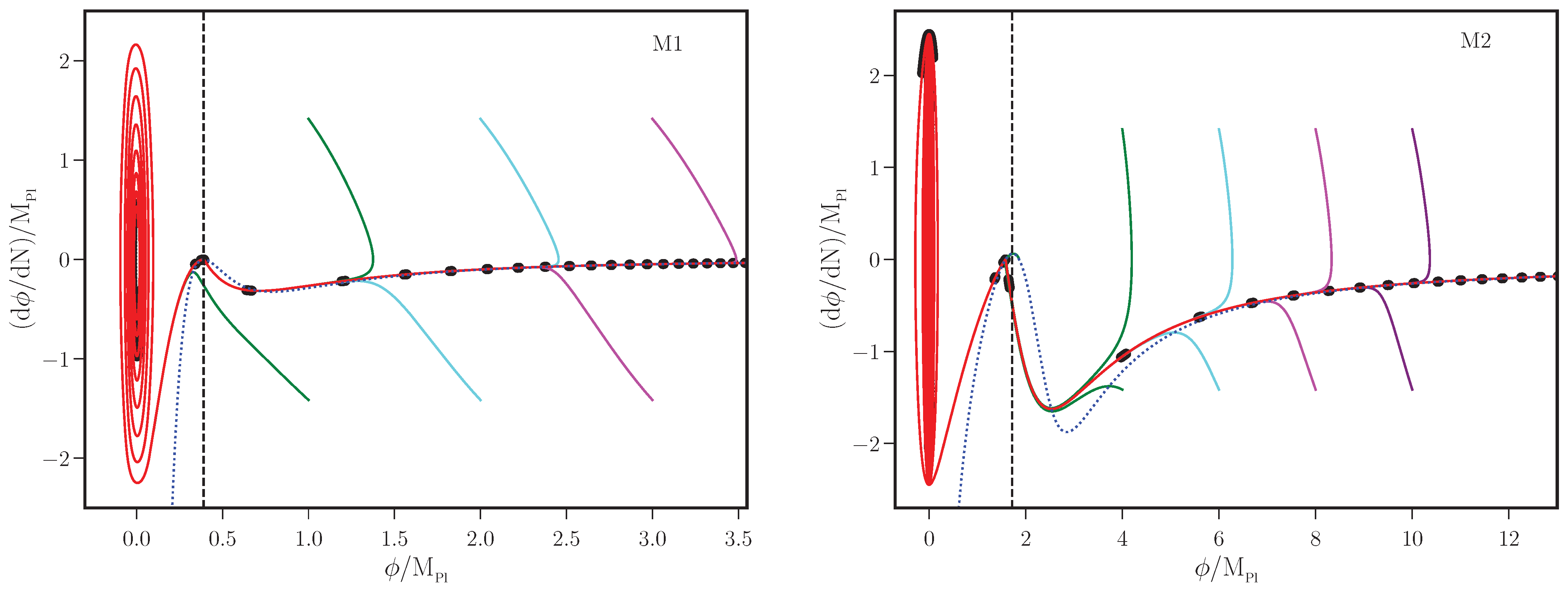
Figure 1. The portrait of the scalar field in the phase space has been illustrated for the two models M1 and M2 (on the left and the right, respectively). We have plotted the trajectories for different initial conditions (as solid curves in different colors), along with the specific initial conditions (plotted in red) that we shall be focusing on in our later discussion. For the initial conditions apart from the ones of our interest, we have considered two values of ϕ N i for each value of ϕ i (plotted in same color). In the case of the primary trajectory, we have indicated the lapse in time every two e-folds (as black dots on the red curves). We have identified the point of inflection (with black vertical lines) and we have also illustrated the evolution arrived at using the standard slow roll approximation (as dotted blue curves).
Galaxies 11 00034 g001
Figure 2. The behavior of the first two slow roll parameters ϵ 1 (on top) and ϵ 2 (at the bottom) have been plotted for the models M1 to M3 (on the left) and for M4 to M6 (on the right). In these plots, we have indicated the values of ϵ 1 = 1 and ϵ 2 = 6 (in dashed black). We should point out that, when ϵ 1 crosses unity, inflation is either interrupted (provided ϵ 1 returns to a value smaller than one soon after) or terminated (if it does not). Note that the value of ϵ 2 = 6 corresponds to the case wherein V ϕ vanishes identically, a point we have discussed in the text.
Galaxies 11 00034 g002
Figure 3. The scalar power spectrum P S ( k ) (in solid lines) and the tensor power spectrum P T ( k ) (in dashed lines) that arise in the models M1 to M6 have been plotted for the parameters and initial conditions that we have discussed. As expected, all the scalar power spectra exhibit a strong peak on small scales due to the epoch of ultra slow roll inflation that occurs in these models.
Galaxies 11 00034 g003
Figure 4. The behavior of the first two slow roll parameters ϵ 1 (on top) and ϵ 2 (at the bottom) are presented for the scenario wherein ϵ 1 ( N ) is given by Equation (33). We have plotted the slow roll parameters over a range of N 1 varied in steps of two e-folds (on the left) and Δ N 1 (on the right). While the effects of the variation in N 1 are evident in the figure, the effects of the variation of Δ N 1 are not so visible. Hence, we have included insets (on the right) to highlight the minor differences that arise in the parameters. Clearly, the slow roll parameters in the reconstructed scenario behave broadly in the same fashion as in the six, specific inflationary models we have considered.
Galaxies 11 00034 g004
Figure 5. The scalar power spectra P S ( k ) (in solid lines) and the tensor power spectra P T ( k ) (in dashed lines) that arise in the reconstructed scenario have been plotted for a range of N 1 (on top) and Δ N 1 (at the bottom). It should be clear (from the figure on top) that, earlier the onset of ultra slow roll, broader is the peak in the scalar power spectra. Also, for the effects due to the variation in Δ N 1 to be distinguishable, we have illustrated (in the figure at the bottom) the relative change in the scalar power spectrum with respect to the spectrum corresponding to the maximum value of Δ N 1 that we have considered (viz. Δ N 1 = 0.320 ). We have also indicated the wave number where the peak is located in the spectra (in dashed black). We find that, for a given value of N 1 (in this case, N 1 = 41 ), a reduction in Δ N 1 leads to an increase in the amplitude of power over the range containing the rise and the peak in the spectrum.
Galaxies 11 00034 g005
Figure 6. The variance σ 2 ( M ) of the density fluctuations has been plotted as a function of the mass M of the PBHs for the inflationary models M1 to M6.
Galaxies 11 00034 g006
Figure 7. The fraction of PBHs f PBH ( M ) that constitute the cold dark matter density in the current universe has been plotted for the inflationary models of interest. We had mentioned that the quantity f PBH ( M ) is very sensitive to the value of δ c . We find that, for the choice of δ c = 0.45 , it is only the inflationary models M2 and M6 that lead to substantial formation of PBHs. In the figure, we have also included the constraints from the different observations, corresponding to a monochromatic spectrum of PBHs.
Galaxies 11 00034 g007
Figure 8. The quantity f PBH ( M ) that arises in the reconstructed scenario has been plotted for different values of N 1 (on the left) and Δ N 1 (on the right). As N 1 is varied, we find that the peaks of f PBH ( M ) behave as M 1 / 2 (indicated in dashed teal) for reasons explained in the text. The increase in Δ N 1 , with a fixed value of N 1 = 41 , results in drastic reduction in the amplitude of f PBH (as shown in the figure on the right). This can be attributed to the fact that an increase in Δ N 1 leads to a gentler transition from slow roll to ultra slow roll inflation, and hence to a smaller height of the peak in the power spectrum. We have also included the constraints from the different observations, as in the previous figure. Note that the quantity f PBH ( M ) depends exponentially on the amplitude of the scalar power spectrum. Hence, despite the wide peaks in the scalar power spectra (cf. Figure 5), the shape of f PBH ( M ) proves to be rather narrow. Due to this reason, we believe that the constraints for the monochromatic power spectra (which we have indicated in the figure) also apply well to the situations of our interest.
Galaxies 11 00034 g008
Figure 9. The dimensionless spectral density of secondary gravitational waves today, viz. Ω GW ( f ) , arising in the inflationary models M1 to M6 has been plotted as function of the frequency f. On the top part of the figure, we have also included the sensitivity curves of the various ongoing and forthcoming GW observatories. It is clear that, in all the models we have considered, the strengths of the secondary GWs are comparable to the sensitivity curves of one or more of the observatories suggesting that it should be possible to detect such signals in the future.
Galaxies 11 00034 g009
Figure 10. The dimensionless spectral density of secondary GWs Ω GW ( f ) that arise in the reconstructed scenario has been plotted for a range of N 1 (on the left) and Δ N 1 (on right). Clearly, smaller the N 1 , longer is the epoch of ultra slow roll and wider is the peak in Ω GW ( f ) . In contrast, the variation in Δ N 1 (at least over the range we have considered) does not alter the shape of Ω GW ( f ) appreciably. We should mention that these spectra of different shapes are consistent with the current bounds on on h 2 Ω GW due to BBN. Even for the spectrum with widest of peaks, upon integration over all frequencies, the dimensionless density of GWs turns out to be about 1.40 × 10 8 . This value is substantially lower than the corresponding BBN bound of around 10 6 (in this context, see, for instance, Refs. [143,144]).
Galaxies 11 00034 g010
Figure 11. The behavior of the bispectrum G ( k 1 , k 2 , k 3 ) in the equilateral and squeezed limits have been plotted (on the left and right, respectively) for the two inflationary models M2 and M3 (in blue and green). We have chosen these models since they exhibit a sharp or a broad peak in their power spectra. Upon comparison with Figure 3, it is evident that the bispectra closely mimic the shapes of the corresponding power spectra. Note that, at small scales, the amplitudes of the bispectra are considerably higher in the equilateral limit than in the squeezed limit.
Galaxies 11 00034 g011
Figure 12. The behavior of the scalar non-Gaussianity parameter f NL ( k 1 , k 2 , k 3 ) has been presented as a density plot for the inflationary models M2 (in the top row) and M3 (in the bottom row). In arriving at these figures, we have chosen the value of k 3 to be k * (i.e., the pivot scale, on the left) or k peak (viz. the location of the peak in the scalar power spectrum, on the right). It should be clear from the density plots that the non-Gaussianity parameter is equilateral in shape near k * (i.e., over the CMB scales, indicating the slow roll evolution of the background during the early stages of inflation), whereas it is highly local in shape around k peak (i.e., on small scales, reflecting the ultra slow roll behavior of the background during the later stages of inflation).
Galaxies 11 00034 g012
Table 1. The scalar spectral index n S and tensor-to-scalar ratio r, evaluated at the pivot scale of k * = 0.05 Mpc 1 , are tabulated for the models M1 to M6. We have also listed the values of N * for the different models that we have worked with to achieve the n S and r mentioned below. Note that, apart from the case of M3, the other models lead to n S and r that are fairly inconsistent with the CMB data.
ModelsM1M2M3M4M5M6
N * 505570505050
n S 0.945 0.946 0.956 0.933 0.936 0.940
r 0.015 0.244 0.041 0.011 0.012 0.017
Disclaimer/Publisher’s Note: The statements, opinions and data contained in all publications are solely those of the individual author(s) and contributor(s) and not of MDPI and/or the editor(s). MDPI and/or the editor(s) disclaim responsibility for any injury to people or property resulting from any ideas, methods, instructions or products referred to in the content.