Abstract
Recently, using Bayesian Machine Learning, a deviation from the cold dark matter model on cosmological scales has been put forward. Such a model might replace the proposed non-gravitational interaction between dark energy and dark matter, and help solve the tension problem. The idea behind the learning procedure relies on a generated expansion rate, while the real expansion rate is just used to validate the learned results. In the present work, however, the emphasis is put on a Gaussian Process (GP), with the available data confirming the possible existence of the already learned deviation. Three cosmological scenarios are considered: a simple one, with an equation-of-state parameter for dark matter , and two other models, with corresponding parameters and . The constraints obtained on the free parameters and hint towards a dynamical nature of the deviation. The dark energy dynamics is also reconstructed, revealing interesting aspects connected with the tension problem. It is concluded, however, that improved tools and more data are needed, to reach a better understanding of the reported deviation.
1. Introduction
The tension problem is presently a hot topic in cosmology. The problem is to understand why the Planck CMB data analysis and a local measurement from the Hubble Space Telescope give different values for . More specifically, it must be understood why in the CDM scenario the Planck CMB data analysis gives km/s/Mpc, while local measurements from the Hubble Space Telescope yield km/s/Mpc [1,2,3,4]. The various mechanisms proposed to explain this unexpected discrepancy need to be understood, yet. There is even a hint that the CDM model could be challenged (see [5,6,7] and references therein for more discussion). However, one should stress that, at this stage of research, it is not clear yet if there is a need for new physics or if everything comes from an overseen mistake on the measurement side.
An attempt to challenge the CDM model was actually in place long before the tension problem appeared. Recall, in particular, the theoretical and conceptual problems caused by the cosmological constant issue, requiring either a modification of general relativity or a consideration of dynamical dark energy models. Indeed, crafting modified theories of gravity and dynamical dark energy models has a relatively long and successful history and plays a crucial role in modern cosmology. In both cases, a workable model can be designed in various ways, for instance, by considering non-gravitational interactions. Alternatively, one can avoid them and use instead a dynamical equation-of-state parameter for dark energy. On top of that, a non-gravitational interaction allows to alleviate or even solve various problems, and, recently, it has been demonstrated that the tension problem may be put among them. Besides all this, reasonable hope is coming from observational data, but from where exactly is it coming is not clear yet [5,6,7,8,9,10,11,12,13,14,15,16,17,18,19,20,21,22,23,24,25,26,27,28,29,30,31,32,33,34,35,36,37,38,39,40,41,42,43,44] (to mention some references covering several aspects of the above-mentioned topics).
Not to mention, the CDM model has a second ingredient, namely, cold dark matter, which could also be a source of tension. But why should the cold dark matter paradigm be challenged? To develop some sort of logic or intuition about this issue, one needs to go back to interacting dark energy models, described by (see, for instance, [12])
and
where and are the dark energy and dark matter energy densities, and and are their pressures, while Q stands for a non-gravitational interaction. The last indicates energy flow between dark energy and dark matter, meaning that their evolution is interconnected and affects each other’s dynamics. We can rewrite Equations (1) and (2) in a slightly different way, as
and
where and are the equation-of-state parameters for dark matter and dark energy, respectively. In this way, we have introduced some effective energy sources where the equation-of-state parameter depends on Q, too. Therefore, even if , we already have an effective non-cold dark matter involved in the dynamics. Moreover, since observational data support , from here, it follows that, by introducing a non-gravitational interaction, we induce corrections to both dark energy and dark matter, which are not in contradiction with the recent observational data. Now, from the above discussion, it seems quite natural to search for possible deviations from the cold dark matter paradigm. It is interesting to study how this approach could solve, or at least alleviate, the already-mentioned tension problems. In particular, it is worthy to discuss the possible impact of the mentioned deviation on the tension problem. Understanding this point is crucial for present-day cosmology since we have seen that this deviation could replace the non-gravitational interaction between these two dark sources, which do not share the same origin and do not operate on the same scales.
Recently, motivated by this possibility, clues for a deviation from the cold dark matter scenario have been gained from a learning procedure, which allowed us to advance towards the solution of the tension problem [6,7]. The learning method was based on a Bayesian (probabilistic) Machine Learning approach and thereby generated expansion rates. In Bayesian Machine Learning, one uses a model-based data generation process to connect physics and our initial belief, to perform the learning. This is a very convenient learning approach that allows one to avoid data-related issues and limitations, and uses instead available data only to validate the learned results. We need to stress that the choice of the initial belief can also be inferred from the data at the very initial step before the learning starts, which gives an idea about ranges where the model parameters could be defined. An alternative option is to use the model itself, supplying some reasonable values to the parameters. In short, we have two different ways to start the learning process, but in any case, the final result should be always validated using real observational data. But this can originate some doubts about the learned results; therefore, it is required—and even constitutes an urgent task—to use more traditional, frequently used tools to first validate and second better understand the learned results.
In the case at hand, we need to study and validate the deviation from the cold dark matter paradigm and understand how this affects the tension problem. To achieve our goal, we use a GP, which is one of the most frequently employed tools in modern cosmology, and it is among the most robust Machine Learning algorithms available.
It is an approach requiring data to be involved, which here will consist of 30 point samples of deduced from the differential age method and 10 data points from the BAO (see Table 1). Recently, this particular tool was used to obtain a model-independent reconstruction of gravity [8]. It has also been employed to study the string swampland criteria in the dark energy-dominated universe, in the case of general relativity and theory of gravity, in [9,10], respectively. Moreover, it has been used in a scalar field potential reconstruction, allowing to constrain any given model revealing its connection to the swampland, among others [11]. In the literature, there are several important applications of this method to study cosmological and astrophysical problems (see [45,46,47,48,49,50,51,52], to mention a few).

Table 1.
and its uncertainty in units of km . The upper panel consists of thirty samples deduced from the differential age method. The lower panel corresponds to ten samples obtained from the radial BAO method. The table is in accordance with [53,54,55,56,57,58,59,60,61,62,63,64,65,66].
In other words, the goal here is to learn and validate a previously learned deviation from the cold dark matter paradigm, using a GP and available expansion rate data (see Table 1). The goal is to reveal possible dynamics in this deviation. Therefore, besides the model with , we have also considered two more models, where the equation-of-state parameter is given by and , respectively. Indeed, the constraints on the free and parameters that we obtain reveal a hint about the dynamical nature of this deviation. On the other hand, using GP, we will reconstruct the dark energy equation-of-state parameter for each of the models considered. The reconstruction allows to reveal various interesting aspects of the dark energy dynamics and hints towards the conclusion that early dark energy could indeed solve the tension problem, among other conclusions.
The present paper is organized as follows. In Section 2, we give some details about GPs, indicating the strategy we have used to investigate a deviation from the cold dark matter model and confirming the recently obtained results where Bayesian Machine Learning was used. The description of the models and the discussion of the results obtained conform Section 3. In the three subsections thereof, the interpretation of the results in each case is explained. Finally, a summarized discussion of the key results of our study, together with some conclusions one can draw from them, is found in Section 4.
2. Gaussian Processes
In this section, a brief presentation of the approach used in the paper is given to gain some intuition about the procedure. The mean, , and the two-point covariance function, , are the key ingredients of a GP, intending to obtain a continuous realization of
and its related uncertainty ; this allows to build the realization region, described by . The last one is the posterior, which will be formed through a Bayesian iterative process. It allows for the reconstruction of the function representing the data in a completely model-independent way, directly from the data. The assumption imposing the data error distribution to be Gaussian is a very important aspect of this method. In other words, we need to consider that the observational data are also a realization of the GP. However, here, the kernel should be chosen manually based on the underlying physics producing the given data.
In the recent literature, the usefulness of various kernels in addressing different issues in cosmology is assessed. Some of the kernels most widely used for this purpose are the squared exponent
the Cauchy kernel
and the Matern () kernel
The and l parameters in Equations (6)–(8) are called the hyperparameters. The l parameter represents the correlation length along which the successive values are correlated, while the parameter is used to control the variation in relative to the mean of the process. The most suitable values of the hyperparameters are determined from the minimization of the GP marginal likelihood. This means that we need to search for the values of the parameters that maximize the probability that the GP generates the considered data. Similarly to other tools, the GPs have advantages and disadvantages that one should not dismiss. As for other Machine Learning (ML) techniques, a GP learns an underlying latent distribution in the data at hand, which strongly affects the learning process too. Therefore, it is not excluded that the algorithm can fail when an unforeseen situation appears. The goal of GP is to infer the features and not visit every single data point to understand why it is there. Because of this, it is possible that it can fail in performing certain tasks or that it will not be able to deal with unforeseen situations, giving sometimes less confident predictions. This aspect should be treated very seriously to avoid misleading results and bad conclusions and consequences. Fortunately, the size of data used in the case of cosmological applications allows for a sensible reduction in the kernel numbers to be considered (as compared to other situations) and also allows us to perform some quick numerical experiments to find where the problem can hide. Readers are invited to check the following references, dealing with how GPs can be used in cosmology, and to learn the necessary mathematics behind this approach [45,46,47,48,49,50,51,52].
Here, we give a short note on the notation to be used (with ). For the metric
and Hubble rate
describing the background dynamics of the universe, the energy conservation law for two energy components reads
and
In the above, and are the dark energy pressure and energy density, while and are the dark matter pressure and energy density, respectively.
In this paper, we take , which together with Equation (12) allows to determine the dark matter energy density dynamics. The last one allows determining the from Equation (10). On the other hand, Equation (11) allows to reconstruct the dark energy pressure, according to
where the prime stands for the derivative with respect to the redshift z. The last equation with allows to reconstruct the dark energy dynamics. In the next section, we will see that, for the three models considered in this paper, only the reconstruction of and is required. This will be performed by using the squared exponential in Equation (6), the Cauchy kernel in Equation (7), and the Matern kernel () in Equation (8). The results hint to (1) a deviation from the cold dark matter model, (2) to the dynamical nature of this deviation, and (3) to an understanding of how this is connected to the tension problem. The details of the strategy being used here will be presented in the next section. As in previous studies, we use the GaPP (Gaussian Processes in Python) package developed by Seikel et al. [67].
3. Models and Results
In this section, we present and discuss the models to be used and the constraints obtained with them. We start with the model with , where is the free parameter to constrain. During the reconstruction, we use the three kernels given by Equations (6)–(8) to understand their differentiated role in the possible deviation from the cold dark matter model. Moreover, with each kernel, we perform the reconstruction assuming three different situations. As a first case, we allow the GP to estimate the value of based on the available expansion rate data, and use it to reconstruct and . In the second case, we set km/s/Mpc together with the expansion rate data and then perform the reconstruction. Finally, in the last case, we take km/s/Mpc followed by the Planck CMB data analysis and, using it with the expansion rate data, we reconstruct and . This strategy allows to gain more intuition about how the deviation from the cold dark matter model can solve the tension problem. To save space, we refer to the upper part of Table 2 to find more about the estimated value for the kernels considered, when just the data given in Table 1 are used in the reconstruction.
Table 2.
Constraints on the parameters for the cosmological model where the deviation from the cold dark matter case is given by Equation (14) and . The constraints are obtained for three kernels, Equations (6), (7), and (8), respectively. The upper part of the table stands for the case when the value is predicted from the GP. In this case, we find , with mean , when the kernel is given by Equation (6). When the kernel corresponds to Equation (7), then with mean . Finally, with mean correspond to the kernel given by Equation (8), respectively. The middle part of the table stands for the case when the value km/s/Mpc from the Hubble Space Telescope is merged with the available expansion rate data given in Table 1 to reconstruct the values of and . Finally, the lower part of the table stands for the case when the km/s/Mpc from the Planck CMB data analysis is merged with the available expansion rate data given in Table 1 and used in the reconstruction.
The reconstruction of and when km/s/Mpc is to be found in Figure 1, in the three cases when the kernel is given by Equation (6) (top panel), by Equation (7) (middle panel), and by Equation (8) (bottom panel), respectively.
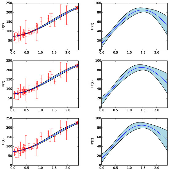
Figure 1.
GPreconstruction of and for the 40-point sample given in Table 1, when reported by the Hubble mission. The top panel depicts the reconstruction when the kernel is that of Equation (6). The middle panel corresponds to the reconstruction from the kernel given by Equation (7). And the bottom panel is the results for the kernel given by Equation (8). The ′ means the derivative with respect to the redshift z.
3.1. Model with
The first model we analyzed using a GP is the one where the dark matter dynamics is given by the following equation:
where and are the Hubble parameter and the fraction of the dark matter at , respectively. This is the model obtained from Equation (12) with and , respectivley. Therefore, for , we will have (see Equation (10))
from where it follows that is given by
After some algebra, for , Equation (13), we obtain
Having and expressed in terms of H and its derivatives, we see that it is possible to study the equation-of-state parameter for dark energy and reveal its nature when one has a deviation from the cold dark matter paradigm. In particular, for the deviation described by Equation (14), for , one obtains
In fact, from the above equations, it follows that, in this case, only the Hubble function H and its first-order derivative are required to be reconstructed. The constraints on the parameters obtained for this case can be found in Table 2. We see that the resulting constraints do hint towards a deviation from the cold dark matter paradigm encoded in the expansion rate data. In particular, for the value obtained for the reconstruction using only the available data given in Table 1, we have already found a hint that there is a deviation from the cold dark matter model (upper part of Table 2).
For the reconstruction of and , we used the value km/s/Mpc coming from the Hubble Space Telescope with the available data and again found a hint that there is a deviation from the cold dark matter model (middle part of Table 2). Eventually, when we used the km/s/Mpc (from the Planck CMB data analysis), we again found a similar hint as in the previous two cases (lower part of Table 2). The strategy used here allowed us to explore and estimate if and how the GP sees a connection between the tension problem and the deviation from the cold dark matter paradigm. In particular, a simple comparison of the constraints we obtained shows that with km/s/Mpc, the deviation from the cold dark matter model should be smaller than when km/s/Mpc. In other words, to solve the tension problem, we need to have a strong deviation from the cold dark matter model according to the expansion rate data. We also noticed that the choice of the kernel can (strongly) affect the constraints on and . However, this does not affect the main conclusion, namely, that we find a deviation from the cold dark matter paradigm on cosmological scales. The results presented in Table 2 hint towards possible new physics and deserve to be treated seriously. On the other hand, this confirms the previously obtained results that were based on Bayesian Machine Learning processes [6].
The reconstruction of and representing the behavior of the dark energy fraction and its equation of state when the kernel is given by Equation (6) can be found in Figure 2 and Figure 3, respectively. For brevity, we will only discuss two cases among all the ones we have studied, with similar qualitative results. They already shed light on the tension problem.
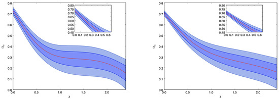
Figure 2.
GP reconstruction of for the model given by Equation (14) and . The plot on the left-hand side corresponds to the reconstruction when km has been merged to the expansion rate data used in the GP and the kernel is given by Equation (6). The right-hand side plot corresponds to the GP reconstruction when km has been merged to the expansion rate data used in the GP and the kernel is given by Equation (6).
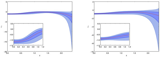
Figure 3.
GP reconstruction of , Equation (18) for the model given by Equation (14) and . The plot on the left-hand side corresponds to the reconstruction when km has been merged to the expansion rate data used in the GP and the kernel is given by Equation (6). In this case, with mean has been found. The right-hand side plot corresponds to the GP reconstruction when km has been merged to the expansion rate data used in the GP and the kernel is given by Equation (6). In this case, with mean has been found.
In Figure 2, the left-hand side plot depicts the reconstructed behavior of the dark energy fraction in a universe where the dark matter dynamics is given by Equation (14). In this case, km/s/Mpc is merged to the data given in Table 1 to be used in the reconstruction. There are various interesting scenarios that the model can reproduce. For instance, we see that in the evolutionary history of such universe, there is an epoch with , which at yields a universe where (according to the lower bound of the reconstruction). On the other hand, according to the upper bound of the reconstruction, there is also a possibility to obtain a model of the universe with an early dark energy component, where the tension problem is solved. In this scenario, at . It should be mentioned that, in the recent literature, early dark energy models have been considered an option to solve the tension problem. According to the mean of the reconstruction at , we expect that , while at , we have a model for the universe where . Moreover, the reconstruction of shows that various starting configurations and evolutionary paths leading to the recent dark energy-dominated universe can be realized within this model. Therefore, it is not surprising that a certain model-dependent parametrization (for instance, of the dark energy equation of state) will not be able to reveal a deviation from the cold dark matter model. Moreover, it is not excluded that similarly, the non-gravitational interaction for a given dark energy model can enter into the dynamics or be removed from the dynamics, respectively. The right-hand side plot of Figure 2 represents the reconstruction when km has been used in the reconstruction process. It indicates that there is a difference in the dynamics of as compared to the previous case, which strongly affects the constraints on at , too. It also affects the dynamics and the constraints on (Figure 3).
The analysis of shows that, with km/s/Mpc, there is an epoch in the history of the universe where dark energy can be in a deep phantom phase but during the evolution can change its nature, becoming quintessence dark energy. On the other hand, it is not excluded that, starting from an , it could evolve and become quintessence dark energy (see the upper bound of the reconstruction on Figure 3, left-hand side plot). We should stress that the analysis of hints that, within the considered scenario, a phantom crossing from above and from below can be realized. Moreover, the analysis of the dark energy equation of state does not reveal any strange or unusual behavior that would exclude a deviation from the cold dark matter model we have considered. During the analysis of this case, we found , with mean , for the kernel given by Equation (6). On the other hand, for the kernel of Equation (7), we obtained , with mean , while , with mean was found for the kernel given by Equation (8), respectively.
For km , we obtained that in the recent universe, the quintessence nature of dark energy is preferable. On the other hand, the phantom crossing from above and from below is still possible. For this case, with mean , for the kernel given by Equation (6). Moreover, for the kernel of Equation (7), we found , with mean , while , with mean , was obtained for the kernel in Equation (8), respectively.
To end the discussion of this model, it should be mentioned that, in all the cases considered, the cosmological constant can be recovered.
3.2. Model with
This second model is considered to investigate the possibility that the deviation from the cold dark matter model has a dynamic nature. We start from the most simple case, namely, the following linear model
The dynamics of this dark matter, given by , are
with
to be used to determine the dark energy pressure . Moreover, after a simple algebra, for and , we have
and
respectively. As a consequence, for the dark energy,
since, from Equation (13), for the pressure , we have
The constraints on , and can be found in Table 3, from which we already see a clear deviation from the cold dark matter model. For this case, we just need now to reconstruct the Hubble function H and its first-order derivative . The constraints on the model parameters—when the value has been obtained during the reconstruction using only the available data given in Table 1—can be found in the upper part of Table 3. The middle part of Table 3 depicts the constraints for the case when, during the reconstruction of and , one merges the km/s/Mpc from the Hubble Space Telescope with the available data. Finally, the lower part of Table 3 corresponds to the constraints in the case when, during the reconstruction, one merges the km/s/Mpc (from the Planck CMB data analysis) with the available data.
Table 3.
Constraints on the parameters for the cosmological model where the deviation from the cold dark matter case is described by Equations (19) and (20), respectively. The constraints are obtained for three kernels, Equations (6), (7), and (8), respectively. The upper part of the table stands for the case when the value is predicted from the GP. In this case, we find , with mean , when the kernel is given by Equation (6). For the kernel given by Equation (7), we find , with mean , while for the kernel given by Equation (8), one obtains with mean , respectively. The middle part of the table stands for the case when km/s/Mpc coming from the Hubble Space Telescope is merged with the available expansion rate data given in Table 1 to reconstruct and . Finally, the lower part of the table stands for the case when km/s/Mpc, from the Planck CMB data analysis, is merged with the available expansion rate data given in Table 1, and then used in the reconstruction.
As a first conclusion, the results indicate a clear deviation from the cold dark matter model and show also that this deviation might have a dynamic nature. Similar to the previous case, we see that for km/s/Mpc, the deviation should be smaller than when km/s/Mpc. However, the considered scenarios, including the kernels, do not affect strongly the constraints on , as it is seen in the case of the first model.
The reconstruction of and , representing the behavior of the dark energy fraction and its equation of state, can be found in Figure 4 and Figure 5, respectively, when the kernel used in the process is given by Equation (6). The left-hand side plot of Figure 4 represents the reconstructed behavior of the dark energy fraction in the universe, where the dark matter dynamics is given by Equation (20), and km/s/Mpc is merged with the data given in Table 1, to be used in the reconstruction. In this case, we find with mean when the kernel is given by Equation (6). Correspondingly, for the kernel given by Equation (7), we find with mean , while with mean is found when the kernel is given by Equation (8), respectively. The right-hand side plot of Figure 4 corresponds to the case when km is used in the reconstruction process. It clearly indicates that, in both cases, there is a difference in the dynamics of , which strongly affects the constraints on and at . Again, we need to stress that the analysis of the dark energy equation of state does not reveal any strange or unusual behavior that would exclude a deviation from the cold dark matter model. The fact that with km in the recent universe, the quintessence nature of dark energy is preferable, can be used to dive deeper into the tension problem, which will be explored using other datasets in forthcoming papers (see the right-hand side plot of Figure 5). In this case, we find with mean , when the kernel is given by Equation (6). When the kernel is that of Equation (7), we find with mean . Finally, with mean is found when the kernel is given by Equation (8). With the deviation from the cold dark matter model here considered, the cosmological constant can be recovered, yet. Indeed, the reconstruction presented in Figure 4 and Figure 5 shows that various scenarios can be reproduced, including early dark energy scenarios, and phantom crossing from above and below, respectively. The scenarios, including the transition between different states of dark energy during the evolution process, are also possible. Here, the cosmological constant can be recovered, too.
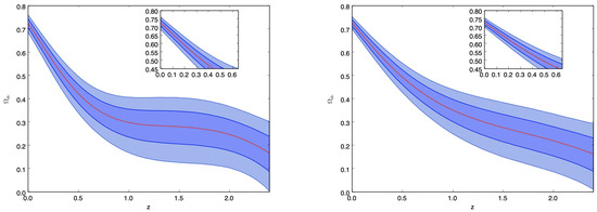
Figure 4.
GP reconstruction of for the model given by Equations (19) and (20). The plot on the left-hand side corresponds to the reconstruction when km is merged with the expansion rate data used in the GP, and the kernel is given by Equation (6). The right-hand side plot corresponds to the GP reconstruction when km is merged with the expansion rate data used in the GP and the kernel is given by Equation (6).
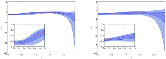
Figure 5.
GP reconstruction of , Equation (24) for the model given by Equations (19) and (20). The plot on the left-hand side corresponds to the reconstruction when km is merged with the expansion rate data used in the GP, and the kernel is given by Equation (6). In this case, one obtains , with mean . The right-hand side plot corresponds to the GP reconstruction when km is merged with the expansion rate data used in the GP, and the kernel is given by Equation (6). In this case, the result is with mean .
3.3. Model with
The last model we analyzed should be seen as a further attempt to reveal the dynamic nature of the deviation, in this case, through a non-linear model. The dark matter equation-of-state parameter has the following form:
and the dark energy state equation reads
because, for the dark energy density dynamics according to Equation (13), we already have
given that . The constraints on , and can be found in Table 4. In this case, too, we need only reconstruct the Hubble function H and its first-order derivative . The constraints on the model parameters, when is obtained during the reconstruction using only the available data given in Table 1, can be found in the upper part of Table 4. The middle part of Table 4 represents the constraints when, during the reconstruction of and , we merge the km/s/Mpc from the Hubble Space Telescope with the available data. Finally, the lower part of Table 4 depicts the constraints when, during the reconstruction, the km/s/Mpc (from the Planck CMB data analysis) is merged with the available data. In this case, too, the constraints we obtained indicate a deviation from the cold dark matter model. And, similar to the previous cases, with km/s/Mpc, the deviation looks to be smaller than when km/s/Mpc.
Table 4.
Constraints on the parameters for the cosmological model where the deviation from the cold dark matter is described by Equations (26) and (28), respectively. The constraints are obtained for three kernels, Equations (6)–(8), and for three different values of the parameter . The upper part of the table stands for the case when the value of is predicted from a GP. In this case, we find , with mean , for the case when the kernel is given by Equation (6). For the kernel given by Equation (7), we have , with mean , while with mean are the results when the kernel is given by Equation (8), respectively. The middle part of the table stands for the case when km/s/Mpc from the Hubble Space Telescope and the available expansion rate data given in Table 1 are merged to reconstruct and . Finally, the lower part of the table stands for the case when km/s/Mpc, coming from the Planck CMB data analysis, is used in the reconstruction.
The reconstruction of and , representing the behavior of the dark energy fraction and its equation of state for this model, are given in Figure 6 and Figure 7, respectively, when the kernel used in the process is the one of Equation (6). The left-hand side plot in Figure 6 corresponds to the reconstructed behavior of the dark energy fraction in the universe, where the dark matter dynamics is that of Equation (20), and km/s/Mpc is merged with the data given in Table 1 to be used in the reconstruction. In this case, we find with mean , when the kernel is given by Equation (6). For the kernel in Equation (7), we have with mean , and for the kernel of Equation (8), , with mean .
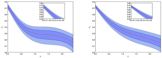
Figure 6.
GP reconstruction of for 30 samples of deduced from the differential age method with 10 additional samples obtained from the radial BAO method (Table 1), when the model is given by Equations (26) and (28). The plot on the left-hand side represents the reconstruction when km is merged with the expansion rate data used in the GP, and the kernel is given by Equation (6). The right-hand side plot corresponds to the GP reconstruction when km is merged with the expansion rate data used in the GP, and the kernel is given by Equation (6).
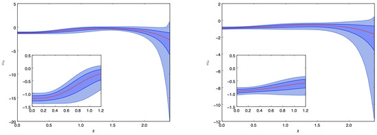
Figure 7.
GP reconstruction of , Equation (27), for the 30 samples deduced from the differential age method with 10 additional samples obtained from the radial BAO method (Table 1), when the model is given by Equations (26) and (28). The plot on the left-hand side represents the reconstruction when km is merged with the expansion rate data used in the GP, and the kernel is given by Equation (6). In this case, , with mean , is found. The right-hand side plot corresponds to the GP reconstruction when km is merged with the expansion rate data used in the GP and the kernel is given by Equation (6). In this case, we obtain with mean .
The right-hand side plot of Figure 6 is the result of the reconstruction when the value km is used in the reconstruction process. Among other results that will be shortly presented below, we find that with mean for the kernel given by Equation (6); with mean for the kernel of Equation (7); and with mean is found for the kernel given by Equation (8), respectively. Results clearly indicate that, in both cases, there is a difference in the dynamics of , which strongly affects the constraints on and at , too. The analysis of shows that for km/s/Mpc in the history of the universe, there is an epoch where dark energy can be in a deep phantom phase but during the evolution change its nature, becoming quintessence dark energy. The model here considered allows for the realization of different scenarios, similarly to previous cases. The reconstructions obtained clearly point out qualitative similarities to the previous cases, which have already been discussed.
To finish this section, we need to stress that choosing a preferable model among the ones considered, by just using a GP and expansion rate data, is indeed a hard process. Additional statistical tools should be applied to perform the model selection with guarantees. More work in this promising direction is needed as will be discussed in the next Section 4.
4. Discussion
In this paper, we use GPs to reveal a possible connection between the tension problem and its solution in terms of a deviation from the cold dark matter model. This extends previous work, where hints about such a deviation were obtained using a Bayesian Machine Learning approach. There, the learning method was based on the generated expansion rate, which already indicated that a deviation from the cold dark matter paradigm might solve the problem. Moreover, a sound possibility that the mentioned deviation could replace a proposed non-gravitational interaction between dark energy and dark matter was also put forward (see [6,7]). In this regard, a mere deviation from the cold dark matter paradigm may be considered more natural, instead of having to rely on a mechanism that generates an interaction between two energy sources, which have different acting scales and roles in our universe.
Improving that work, we here use a pure GP and real, available expansion rate data, at the expense of significantly restricting the redshift range of the analysis. The results in this case are far more reliable, and we need to stress that, despite the restricted range, here, hints indicating a deviation from the cold dark matter model are distinctly inferred. In our analysis, we use 40-point data consisting of 30-point samples deduced from the differential age method and 10-point samples obtained from the radial BAO method. Already in this prospective situation, we have found a hint that the deviation from the cold dark matter paradigm could be a source for the tension problem. Moreover, we have learned that, when the deviation is described by a free parameter, , to solve the tension problem, we would need quite a strong deviation from the cold dark matter model.
The consideration of the other two models with has confirmed this connection. Using three different kernels and three different values for the parameter, we have been able to reveal that an early dark energy component may solve the tension problem. In this case, the early dark energy model originates from the mentioned deviation, without the need to introduce auxiliary dark energy models or non-gravitational interactions of any sort. On the other hand, we have also learned, from the reconstruction, that phantom crossing from above (and/or from below) can be used to craft a solution for the tension problem, too.
For km , an indication that the quintessence nature of dark energy is preferable has been obtained. We should also stress the fact that, in all cases under study, the cosmological constant could be recovered, with the independence of the chosen scenario deployed in our study. It is not in accordance with the mean of the reconstruction; therefore, we have a hint that the tension still indicates a problem with the physics, indeed.
Finally, we should stress once more that the behavior we have obtained for (and , too) and for does not contain any indication that the deviation from the cold dark matter model is an artifact originating in the procedure employed itself. Rather, the results of the present study provide a clear image of the fact that the deviation is indeed imprinted into the observational expansion rate data. What is more, we prove that the deviation can most likely have a dynamical component, and two possibilities thereof have been explored.
The results here obtained, combined with the ones reported in [6], provide support for an interesting, alternative way to approach the solution to various fundamental problems of modern cosmology. They already support the idea of extending the analysis in various directions. The most important issue would be to understand how the deviation from the cold dark matter model affects structure formation in our universe. It is key to understand, in particular, how it may affect the constraints on neutrino physics and help (or prevent) a unified treatment of dark energy and dark matter. Also, a better understanding of how, within the discussed scenario, non-gravitational interactions could be suppressed in cosmological models is another interesting issue deserving consideration.
Author Contributions
Conceptualization, M.K. and E.E.; methodology, M.K.; software, M.K.; validation, E.E. and M.K.; writing—original draft preparation, M.K. and E.E; writing—review and editing, M.K. and E.E. All authors have read and agreed to the published version of the manuscript.
Funding
M.K. has been supported by a Juan de la Cierva-incorporación grant (IJC2020-042690-I). This research was funded by MICINN (Spain), project PID2019-104397GB-I00 of the Spanish State Research Agency program AEI/10.13039/501100011033, CSIC project 2024AEP171, by the Catalan Government AGAUR project 2021-SGR-00171, and by the program Unidad de Excelencia María de Maeztu CEX2020-001058-M.
Data Availability Statement
Data is contained within the article.
Acknowledgments
The authors are indebted with the referees for relevant comments and suggestions, which helped to improve the paper.
Conflicts of Interest
The authors declare no conflicts of interest.
References
- Planck Collaboration; Aghanim, N.; Akrami, Y.; Ashdown, M.; Aumont, J.; Baccigalupi, C.; Ballardini, M.; Banday, A.J.; Barreiro, R.B.; Bartolo, N.; et al. Planck 2018 results. VI. Cosmological parameters. Astron. Astrophys. 2020, 641, A6. [Google Scholar] [CrossRef]
- Riess, A.G.; Casertano, S.; Yuan, W.; Macri, L.; Bucciarelli, B.; Lattanzi, M.G.; MacKenty, J.W.; Bowers, J.B.; Zheng, W.; Filippenko, A.V. Milky Way Cepheid Standards for Measuring Cosmic Distances and Application to Gaia DR2: Implications for the Hubble Constant. Astrophys. J. 2018, 861, 126. [Google Scholar] [CrossRef]
- Wong, K.C.; Suyu, S.H.; Chen, G.C.-F.; Rusu, C.E.; Millon, M.; Sluse, D.; Bonvin, V.; Fassnacht, C.D.; Taubenberger, S.; Auger, M.W.; et al. H0LiCOW XIII. A 2.4% measurement of H0 from lensed quasars: 5.3σ tension between early and late-Universe probes. Mon. Not. R. Astron. Soc. 2020, 498, 1420. [Google Scholar] [CrossRef]
- Freedman, W.L.; Madore, B.F.; Hatt, D.; Hoyt, T.J.; Jang, I.S.; Beaton, R.L.; Burns, C.R.; Lee, M.G.; Monson, A.J.; Neeley, J.R.; et al. The Carnegie-Chicago Hubble Program. VIII. An Independent Determination of the Hubble Constant Based on the Tip of the Red Giant Branch. ApJ 2019, 882, 34. [Google Scholar] [CrossRef]
- Perivolaropoulos, L.; Skara, F. Challenges for LambaCDM: An update. New Astron. Rev. 2022, 95, 101659. [Google Scholar] [CrossRef]
- Elizalde, E.; Gluza, J.; Khurshudyan, M. An approach to cold dark matter deviation and the H0 tension problem by using machine learning. arXiv 2021, arXiv:2104.01077. [Google Scholar] [CrossRef]
- Khurshudyan, M. Swampland Criteria and Neutrino Generation in a Non-Cold Dark Matter Universe. Astrophysics 2023, 66, 423–440. [Google Scholar] [CrossRef]
- Cai, Y.F.; Khurshudyan, M.; Saridakis, E.N. Model-independent reconstruction of f(T) gravity from Gaussian Processes. Astrophys. J. 2020, 888, 62. [Google Scholar] [CrossRef]
- Elizalde, E.; Khurshudyan, M. Swampland criteria for a dark energy dominated universe ensuing from Gaussian processes and H(z)data analysis. Phys. Rev. D 2019, 99, 103533. [Google Scholar] [CrossRef]
- Elizalde, E.; Khurshudyan, M. Swampland criteria for f(R) gravity derived with a Gaussian process. Eur. Phys. J. C 2022, 82, 811. [Google Scholar] [CrossRef]
- Elizalde, E.; Khurshudyan, M.; Myrzakulov, K.; Bekov, S. Reconstruction of the quintessence dark energy potential from a Gaussian process. arXiv 2022, arXiv:2203.06767. [Google Scholar] [CrossRef]
- Aljaf, M.; Elizalde, E.; Khurshudyan, M.; Myrzakulov, K.; Zhadyranova, A. Solving the tension in f(T) gravity through Bayesian machine learning. Eur. Phys. J. C 2022, 82, 1130. [Google Scholar] [CrossRef]
- Yerzhanov, K.; Myrzakul, S.; Kenzhalin, D.; Khurshudyan, M. Interacting ω(q) dark energy model with phase space analysis. Mod. Phys. Lett. A 2021, 36, 2150222. [Google Scholar] [CrossRef]
- Aljaf, M.; Grigoris, D.; Khurshudyan, M. Assessing the foundation and applicability of some dark energy fluid models in the Dirac-Born-Infeld framework. Int. J. Mod. Phys. A 2022, 37, 2250211. [Google Scholar] [CrossRef]
- Elizalde, E.; Khurshudyan, M. Interplay between Swampland and Bayesian Machine Learning in constraining cosmological models. Eur. Phys. J. C 2021, 81, 335, Erratum in Eur. Phys. J. C 2021, 81, 438. [Google Scholar] [CrossRef]
- Elizalde, E.; Khurshudyan, M. Constraints on cosmic opacity from Bayesian machine learning: The hidden side of the H0tension problem. Phys. Dark Univ. 2022, 37, 101114. [Google Scholar] [CrossRef]
- Elizalde, E.; Khurshudyan, M.; Odintsov, S.D. Analysis of the H0 tension problem in the Universe with viscous dark fluid. Phys. Rev. D 2020, 102, 123501. [Google Scholar] [CrossRef]
- Elizalde, E.; Khurshudyan, M.; Nojiri, S. Cosmological singularities in interacting dark energy models with an ω(q) parametrization. Int. J. Mod. Phys. D 2019, 28, 1950019. [Google Scholar] [CrossRef]
- Khurshudyan, M.; Myrzakulov, R. Phase space analysis of some interacting Chaplygin gas models. Eur. Phys. J. C 2017, 77, 65. [Google Scholar] [CrossRef]
- Li, C.; Ren, X.; Khurshudyan, M.; Cai, Y.-F. Implications of the possible 21-cm line excess at cosmic dawn on dynamics of interacting dark energy. Phys. Lett. B 2020, 80, 135141. [Google Scholar] [CrossRef]
- Wang, B.; Abdalla, E.; Atrio-Barandela, F.; Pavon, D. Further understanding the interaction between dark energy and dark matter: Current status and future directions. arXiv 2024, arXiv:2402.00819. [Google Scholar] [CrossRef] [PubMed]
- Linden, S.; Virey, J.-M. Test of the Chevallier-Polarski-Linder parametrization for rapid dark energy equation of state transitions. Phys. Rev. D 2008, 78, 023526. [Google Scholar] [CrossRef]
- Odintsov, S.D.; Oikonomou, V.K.; Tretyakov, P.V. Phase space analysis of the accelerating multifluid Universe. Phys. Rev. D 2017, 96, 044022. [Google Scholar] [CrossRef]
- Bamba, K.; Capozziello, S.; Nojiri, S.; Odintsov, S.D. Dark energy cosmology: The equivalent description via different theoretical models and cosmography tests. Astrophys. Space Sci. 2012, 342, 155. [Google Scholar] [CrossRef]
- Yang, W.; Pan, S.; Vagnozzi, S.; Valentino, E.D.; Mota, F.D.; Capozziello, S. Dawn of the dark: Unified dark sectors and the EDGES Cosmic Dawn 21-cm signal. J. Cosmol. Astropart. Phys. 2019, 1911, 044. [Google Scholar] [CrossRef]
- Yang, W.; Pan, S.; Valentino, E.D.; Saridakis, E.N.; Chakraborty, S. Observational constraints on one-parameter dynamical dark-energy parametrizations and the H0 tension. Phys. Rev. D 2019, 99, 043543. [Google Scholar] [CrossRef]
- Elizalde, E.; Khurshudyan, M. Cosmology with an interacting van der Waals fluid. Int. J. Mod. Phys. D 2018, 27, 1850037. [Google Scholar] [CrossRef]
- Aljaf, M.; Gregoris, D.; Khurshudyan, M. Phase space analysis and singularity classification for linearly interacting dark energy models. Eur. Phys. J. C 2020, 80, 112. [Google Scholar] [CrossRef]
- Sadri, E.; Khurshudyan, M.; Zeng, D.-F. Scrutinizing various phenomenological interactions in the context of holographic Ricci dark energy models. Eur. Phys. J. C 2020, 80, 393. [Google Scholar] [CrossRef]
- Amirhashchi, H.; Yadav, A.K.; Ahmad, N.; Yadav, V. Interacting Dark Sectors in Anisotropic Universe: Observational Constraints and H0 Tension. Phys. Dark Universe 2022, 36, 101043. [Google Scholar] [CrossRef]
- Alestas, G.; Kazantzidis, L.; Perivolaropoulos, L. H0 Tension, Phantom Dark Energy and Cosmological Parameter Degeneracies. Phys. Rev. D 2020, 101, 123516. [Google Scholar] [CrossRef]
- Wang, D.; Mota, D. Can f(T) gravity resolve the H0 tension? Phys. Rev. D 2020, 102, 063530. [Google Scholar] [CrossRef]
- Blinov, N.; Keith, C.; Hooper, D. Warm Decaying Dark Matter and the Hubble Tension. J. Cosmol. Astropart. Phys. 2020, 6, 005. [Google Scholar] [CrossRef]
- Li, E.K.; Du, M.; Zhou, Z.-H.; Zhang, H.; Xu, L. Testing the effect of H0 on fσ8 tension using a Gaussian Process method. MNRAS 2021, 501, 4452–4463. [Google Scholar] [CrossRef]
- Valentino, E.D.; Melchiorri, A.; Mena, O.; Vagnozzi, S. Nonminimal dark sector physics and cosmological tensions. Phys. Rev. D 2020, 101, 063502. [Google Scholar] [CrossRef]
- Valentino, E.D.; Mukherjee, A.; Sen, A.A. Dark Energy with Phantom Crossing and the H0 tension. Entropy 2021, 23, 404. [Google Scholar] [CrossRef] [PubMed]
- Nunes, R.C. Structure formation in f(T) gravity and a solution for H0 tension. J. Cosmol. Astropart. Phys. 2018, 5, 052. [Google Scholar] [CrossRef]
- Brevik, I.; Elizalde, E.; Odintsov, S.D.; Timoshkin, A.V. Inflationary universe in terms of a van der Waals viscous fluid. Int. J. Geom. Meth. Mod. Phys. 2017, 14, 1750185. [Google Scholar] [CrossRef]
- Capozziello, S.; D’Agostino, R.; Giambo, R.; Luongo, O. Effective field description of the Anton-Schmidt cosmic fluid. Phys. Rev. D 2019, 99, 023532. [Google Scholar] [CrossRef]
- Nojiri, S.; Odintsov, S.D. Inhomogeneous equation of state of the universe: Phantom era, future singularity, and crossing the phantom barrier. Phys. Rev. D 2005, 72, 023003. [Google Scholar] [CrossRef]
- Brevik, I.; Obukhov, V.V.; Osetrin, K.E.; Timoshkin, A.V. Little rip cosmological models with time dependent equation of state. Mod. Phys. Lett. A 2012, 27, 1250210. [Google Scholar] [CrossRef]
- Brevik, I.; Gron, O.; de Haro, J.; Odintsov, S.D.; Saridakis, E.N. Viscous cosmology for early- and late-time Universe. J. Mod. Phys. D 2017, 26, 1730024. [Google Scholar] [CrossRef]
- Odintsov, S.D.; Oikonomou, V.K.; Timoshkin, A.V.; Saridakis, E.N.; Myrzakulov, R. Cosmological fluids with logarithmic equation of state. Ann. Phys. 2018, 398, 238–253. [Google Scholar] [CrossRef]
- Odintsov, S.D.; Gomez, D.S.-C.; Sharov, G.S. Testing the equation of state for viscous dark energy. Phys. Rev. D 2020, 101, 044010. [Google Scholar] [CrossRef]
- Rin, X.; Yan, S.-F.; Zhao, Y.; Cai, Y.-F.; Saridakis, E.N. Gaussian processes and effective field theory of f(T) gravity under the H0 tension. Astrophys. J. 2022, 932, 131. [Google Scholar] [CrossRef]
- Wu, P.; Qi, J.-Z.; Zhang, X. Null test for cosmic curvature using Gaussian process. Chin. Phys. C 2023, 47, 055106. [Google Scholar] [CrossRef]
- Said, J.L.; Mifsud, J.; Sultana, J.; Adami, K.Z. Reconstructing teleparallel gravity with cosmic structure growth and expansion rate data. J. Cosmol. Astropart. Phys. 2021, 6, 015. [Google Scholar] [CrossRef]
- Gomez-Valent, A.; Amendola, L. H0 from cosmic chronometers and Type Ia supernovae, with Gaussian Processes and the novel Weighted Polynomial Regression method. J. Cosmol. Astropart. Phys. 2018, 1804, 051. [Google Scholar] [CrossRef]
- Dhawan, S.; Alsing, J.; Vagnozzi, S. Non-parametric spatial curvature inference using late-universe cosmological probes. Mon. Not. R. Astron. Soc. 2021, 506, L1. [Google Scholar] [CrossRef]
- Colgain, E.O.; Sheikh-Jabbari, M.M. Elucidating cosmological model dependence with H0. arXiv 2021, arXiv:2101.08565. [Google Scholar] [CrossRef]
- Bernardo, R.C.; Said, J.L. A data-driven Reconstruction of Horndeski gravity via the Gaussian processes. J. Cosmol. Astropart. Phys. 2021, 9, 014. [Google Scholar] [CrossRef]
- Bernardo, R.C.; Said, J.L. Towards a model-independent reconstruction approach for late-time Hubble data. J. Cosmol. Astropart. Phys. 2021, 8, 027. [Google Scholar] [CrossRef]
- Zhang, C.; Zhang, H.; Yuan, S.; Liu, S.; Zhang, T.-J.; Sun, Y.-C. Four new observational H(z) data from luminous red galaxies in the Sloan Digital Sky Survey data release seven. Res. Astron. Astrophys. 2014, 14, 1221. [Google Scholar] [CrossRef]
- Moresco, M.; Pozzetti, L.; Cimatti, A.; Jimenez, R.; Maraston, C.; Verde, L.; Thomas, D.; Citro, A.; Tojeiro, R.; Wilkinson, D. A 6% measurement of the Hubble parameter at z≈0.45: Direct evidence of the epoch of cosmic re-acceleration. J. Cosmol. Astropart. Phys. 2016, 5, 014. [Google Scholar] [CrossRef]
- Jimenez, R.; Verde, L.; Treu, T.; Stern, D. Constraints on the equation of state of dark energy and the Hubble constant from stellar ages and the CMB. Astrophys. J. 2003, 593, 622. [Google Scholar] [CrossRef]
- Stern, D.; Jimenez, R.; Verde, L.; Kamionkowski, M.; Stanford, S.A. Cosmic chronometers: Constraining the equation of state of dark energy. I: H(z) measurements. J. Cosmol. Astropart. Phys. 2010, 2, 008. [Google Scholar] [CrossRef]
- Moresco, M.; Cimatti, A.; Jimenez, R.; Pozzetti, L.; Zamorani, G.; Bolzonella, M.; Dunlop, J.; Lamareille, F.; Mignoli, M.; Pearce, H.; et al. Improved constraints on the expansion rate of the Universe up to z≈1.1 from the spectroscopic evolution of cosmic chronometers. J. Cosmol. Astropart. Phys. 2012, 8, 006. [Google Scholar] [CrossRef]
- Simon, J.; Verde, L.; Jimenez, R. Constraints on the redshift dependence of the dark energy potential. Phys. Rev. D 2005, 71, 123001. [Google Scholar] [CrossRef]
- Moresco, M. Raising the bar: New constraints on the Hubble parameter with cosmic chronometers at z≈2. Mon. Not. R. Astron. Soc. Lett. 2015, 450, L16. [Google Scholar] [CrossRef]
- Gaztanaga, E.; Cabre, A.; Hui, L. Clustering of luminous red galaxies – IV. Baryon acoustic peak in the line-of-sight direction and a direct measurement of H(z). Mon. Not. R. Astron. Soc. 2009, 399, 1663. [Google Scholar] [CrossRef]
- Blake, C.; Brough, S.; Colless, M.; Contreras, C.; Couch, W.; Croom, S.; Croton, D.; Davis, T.M.; Drinkwater, M.J.; Forster, K.; et al. The WiggleZ Dark Energy Survey: Joint measurements of the expansion and growth history at z < 1. Mon. Not. R. Astron. Soc. 2012, 425, 405. [Google Scholar] [CrossRef]
- Xu, X.; Cuesta, A.J.; Padmanabhan, N.; Eisenstein, D.J.; McBride, C.K. Measuring DA and H at z = 0.35 from the SDSS DR7 LRGs using baryon acoustic oscillations. Mon. Not. R. Astron. Soc. 2013, 431, 2834. [Google Scholar] [CrossRef]
- Busca, N.G.; Delubac, T.; Rich, J.; Bailey, S.; Font-Ribera, A.; Kirkby, D.; Le Goff, J.-M.; Pieri, M.M.; Slosar, A.; Aubourg, A.; et al. Baryon acoustic oscillations in the Lyα forest of BOSS quasars*. Astron. Astrophys. 2013, 552, A96. [Google Scholar] [CrossRef]
- Delubac, T.; Bautista, J.E.; Busca, N.G.; Rich, J.; Kirkby, D.; Bailey, S.; Font-Ribera, A.; Slosar, A.; Lee, K.-G.; Pieri, M.M.; et al. Baryon acoustic oscillations in the Lyα forest of BOSS DR11 quasars*. Astron. Astrophys. 2015, 574, A59. [Google Scholar] [CrossRef]
- Samushia, L.; Reid, B.A.; White, M.; Percival, W.J.; Cuesta, A.J.; Lombriser, L.; Manera, M.; Nichol, R.C.; Schneider, D.P.; Bizyaev, D.; et al. The clustering of galaxies in the SDSS-III DR9 Baryon Oscillation Spectroscopic Survey: Testing deviations from λ and general relativity using anisotropic clustering of galaxies. Mon. Not. R. Astron. Soc. 2013, 429, 1514. [Google Scholar] [CrossRef]
- Font-Ribera, A.; Kirkby, D.; Busca, N.; Miralda-Escude, J.; Ross, N.P.; Slosar, A.; Rich, J.; Aubourg, E.; Bailey, S.; Bhardwaj, V.; et al. Quasar-Lyman α Forest Cross-Correlation from BOSS DR11: Baryon Acoustic Oscillations. J. Cosmol. Astropart. Phys. 2014, 5, 027. [Google Scholar] [CrossRef]
- Seikel, M.; Clarkson, C.; Smith, M. Reconstruction of dark energy and expansion dynamics using Gaussian processes. J. Cosmol. Astropart. Phys. 2012, 6, 036. [Google Scholar] [CrossRef]
Disclaimer/Publisher’s Note: The statements, opinions and data contained in all publications are solely those of the individual author(s) and contributor(s) and not of MDPI and/or the editor(s). MDPI and/or the editor(s) disclaim responsibility for any injury to people or property resulting from any ideas, methods, instructions or products referred to in the content. |
© 2024 by the authors. Licensee MDPI, Basel, Switzerland. This article is an open access article distributed under the terms and conditions of the Creative Commons Attribution (CC BY) license (https://creativecommons.org/licenses/by/4.0/).