
LAMOST Spectroscopy and Gaia Photo-Astrometry for an Interstellar Extinction Study


Abstract
1. Introduction
2. Data and Method
2.1. Observational Data
2.2. Estimation of Total Galactic Extinction
2.3. Error Budget
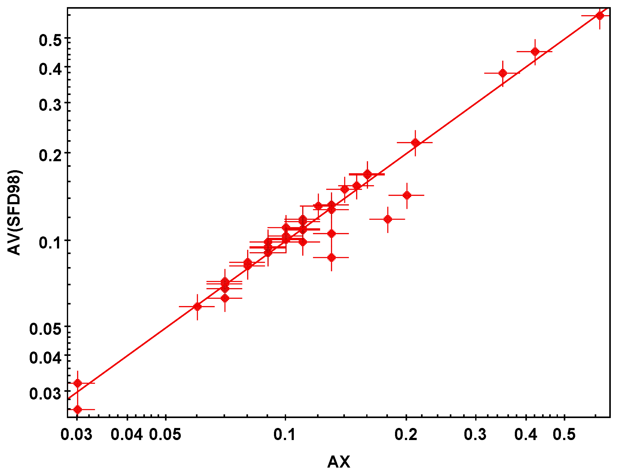
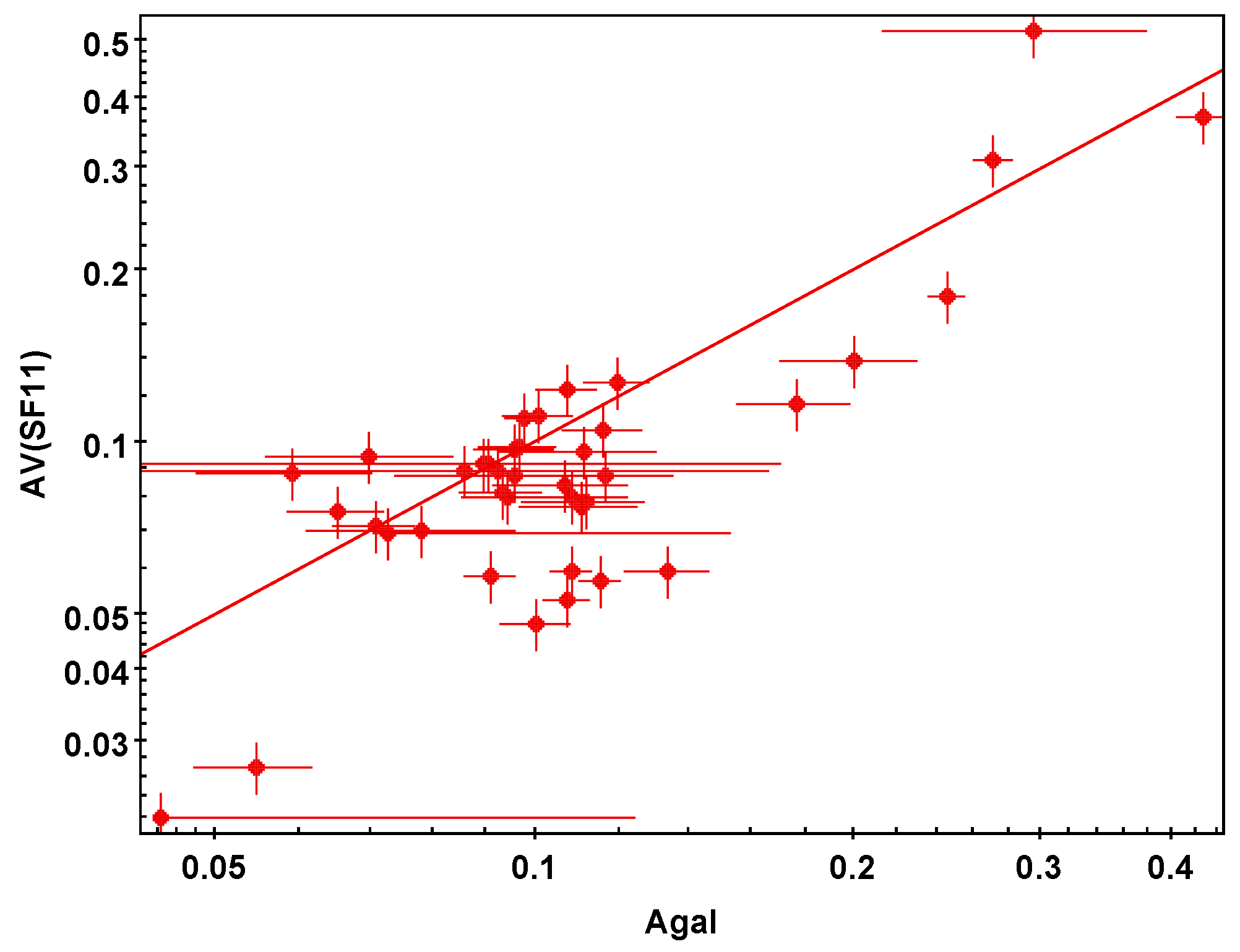
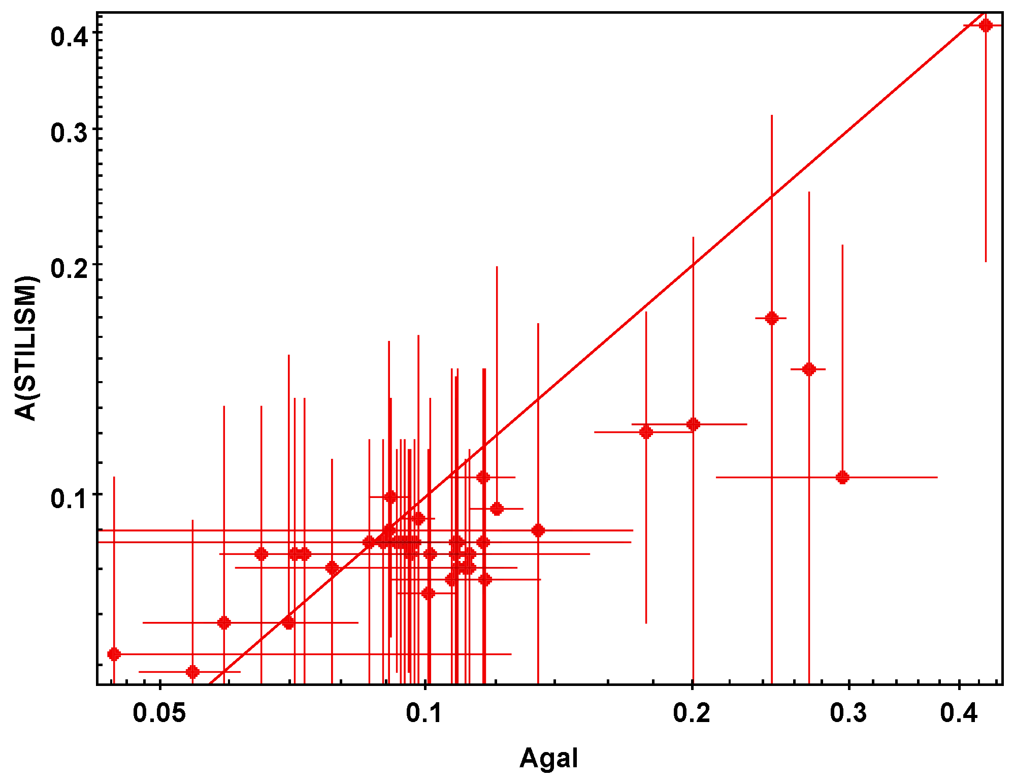
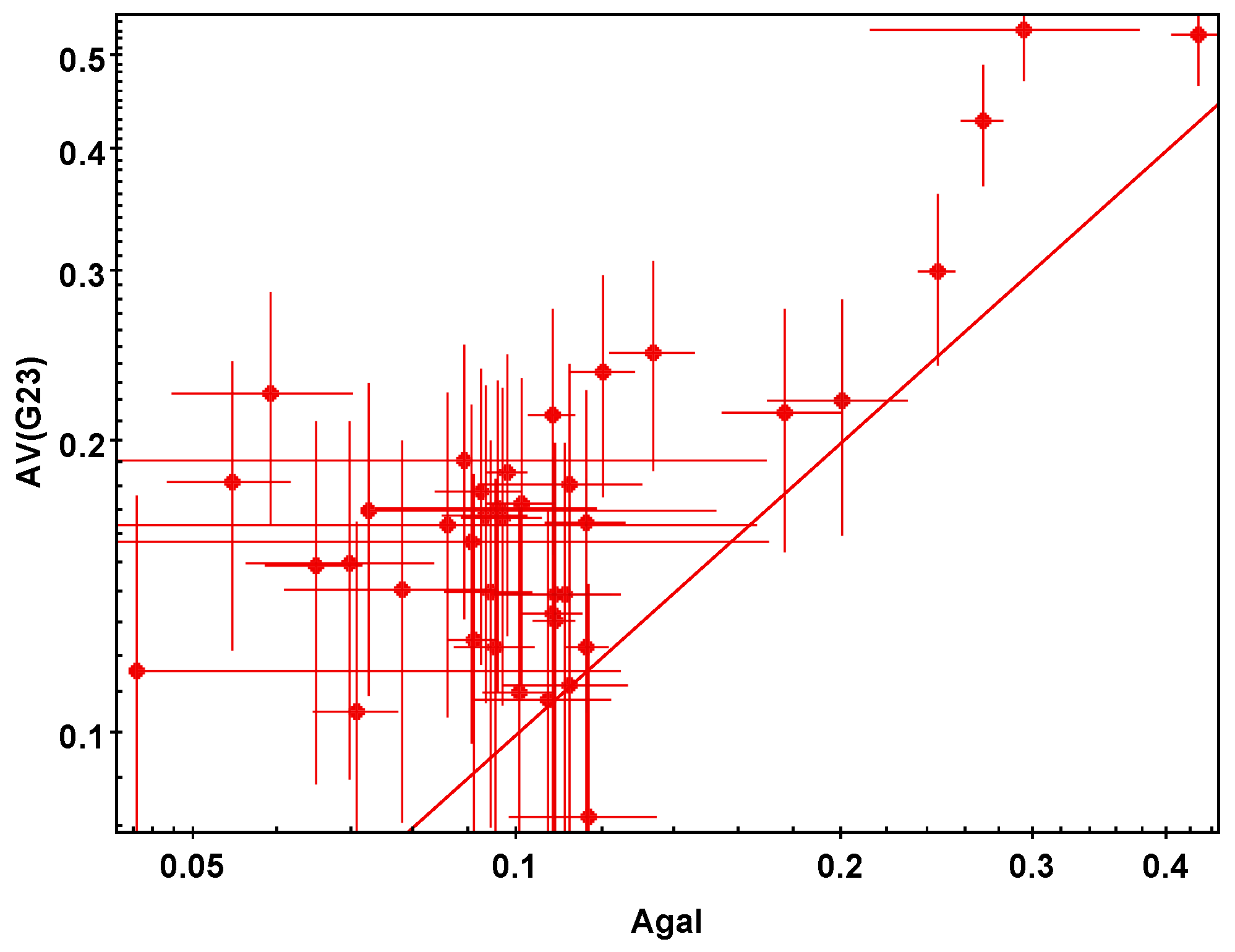
3. Comparison of with Other Maps
3.1. Area Centres
3.2. 2D Maps of Galactic Extinction
3.3. STILISM Service
3.4. G23 Map
4. Conclusions
Author Contributions
Funding
Data Availability Statement
Acknowledgments
Conflicts of Interest
References
- Parenago, P.P. On interstellar extinction of light. Astron. Zh. 1940, 13, 3. [Google Scholar]
- Fitzgerald, M.P. The Distribution of Interstellar Reddening Material. Astron. J. 1968, 73, 983. [Google Scholar] [CrossRef]
- Neckel, T.; Klare, G. The spatial distribution of the interstellar extinction. Astron. Astrophys. Suppl. Ser. 1980, 42, 251. [Google Scholar]
- Pandey, A.K.; Mahra, H.S. Interstellar extinction and Galactic structure. Mon. Not. R. Astron. Soc. 1987, 226, 635–643. [Google Scholar] [CrossRef]
- Arenou, F.; Grenon, M.; Gomez, A. A tridimensional model of the galactic interstellar extinction. Astron. Astrophys. 1992, 258, 104–111. [Google Scholar]
- Gontcharov, G.A. Influence of the Gould belt on interstellar extinction. Astron. Lett. 2009, 35, 780–790. [Google Scholar] [CrossRef]
- Gontcharov, G.A.; Marchuk, A.A.; Khovrichev, M.Y.; Mosenkov, A.V.; Savchenko, S.S.; Il’in, V.B.; Poliakov, D.M.; Smirnov, A.A. New Interstellar Extinction Maps Based on Gaia and Other Sky Surveys. Astron. Lett. 2023, 49, 673–696. [Google Scholar] [CrossRef]
- Sale, S.E.; Drew, J.E.; Barentsen, G.; Farnhill, H.J.; Raddi, R.; Barlow, M.J.; Eislöffel, J.; Vink, J.S.; Rodríguez-Gil, P.; Wright, N.J. A 3D extinction map of the northern Galactic plane based on IPHAS photometry. Mon. Not. R. Astron. Soc. 2014, 443, 2907–2922. [Google Scholar] [CrossRef]
- Lallement, R.; Capitanio, L.; Ruiz-Dern, L.; Danielski, C.; Babusiaux, C.; Vergely, L.; Elyajouri, M.; Arenou, F.; Leclerc, N. Three-dimensional maps of interstellar dust in the Local Arm: Using Gaia, 2MASS, and APOGEE-DR14. Astron. Astrophys. 2018, 616, A132. [Google Scholar] [CrossRef]
- Green, G.M.; Schlafly, E.; Zucker, C.; Speagle, J.S.; Finkbeiner, D. A 3D Dust Map Based on Gaia, Pan-STARRS 1, and 2MASS. Astrophys. J. 2019, 887, 93. [Google Scholar] [CrossRef]
- Chen, B.Q.; Huang, Y.; Yuan, H.B.; Wang, C.; Fan, D.W.; Xiang, M.S.; Zhang, H.W.; Tian, Z.J.; Liu, X.W. Three-dimensional interstellar dust reddening maps of the Galactic plane. Mon. Not. R. Astron. Soc. 2019, 483, 4277–4289. [Google Scholar] [CrossRef]
- Leike, R.H.; Glatzle, M.; Enßlin, T.A. Resolving nearby dust clouds. Astron. Astrophys. 2020, 639, A138. [Google Scholar] [CrossRef]
- Nekrasov, A.; Grishin, K.; Kovaleva, D.; Malkov, O. Approximate analytical description of the high latitude extinction. Eur. Phys. J. Spec. Top. 2021, 230, 2193–2205. [Google Scholar] [CrossRef]
- Brown, A.G.A. et al. [Gaia Collaboration] Gaia Early Data Release 3. Summary of the contents and survey properties. Astron. Astrophys. 2021, 649, A1. [Google Scholar] [CrossRef]
- Luo, A.L.; Zhao, Y.H.; Zhao, G.; Deng, L.C.; Liu, X.W.; Jing, Y.P.; Wang, G.; Zhang, H.T.; Shi, J.R.; Cui, X.Q.; et al. The first data release (DR1) of the LAMOST regular survey. Res. Astron. Astrophys. 2015, 15, 1095. [Google Scholar] [CrossRef]
- Luo, A.L.; Zhao, Y.H.; Zhao, G. VizieR Online Data Catalog: LAMOST DR5 catalogs (Luo+, 2019). In VizieR Online Data Catalog; NASA: Washington, DC, USA, 2019; p. V-164. [Google Scholar]
- Avdeeva, A.; Kovaleva, D.; Malkov, O.; Nekrasov, A. Fitting procedure for estimating interstellar extinction at high galactic latitudes. Open Astron. 2021, 30, 168–175. [Google Scholar] [CrossRef]
- Steinmetz, M. et al. [RAVE Collaboration] The Sixth Data Release of the Radial Velocity Experiment (RAVE). II. Stellar Atmospheric Parameters, Chemical Abundances, and Distances. Astron. J. 2020, 160, 83. [Google Scholar] [CrossRef]
- Burstein, D.; Heiles, C. Reddenings derived from H I and galaxy counts: Accuracy and maps. Astron. J. 1982, 87, 1165–1189. [Google Scholar] [CrossRef]
- Schlegel, D.J.; Finkbeiner, D.P.; Davis, M. Maps of Dust Infrared Emission for Use in Estimation of Reddening and Cosmic Microwave Background Radiation Foregrounds. Astrophys. J. 1998, 500, 525–553. [Google Scholar] [CrossRef]
- Schlafly, E.F.; Finkbeiner, D.P. Measuring Reddening with Sloan Digital Sky Survey Stellar Spectra and Recalibrating SFD. Astrophys. J. 2011, 737, 103. [Google Scholar] [CrossRef]
- Vallenari, A. et al. [Gaia Collaboration] Gaia Data Release 3. Summary of the content and survey properties. Astron. Astrophys. 2023, 674, A1. [Google Scholar] [CrossRef]
- Bailer-Jones, C.A.L.; Rybizki, J.; Fouesneau, M.; Mantelet, G.; Andrae, R. Estimating Distance from Parallaxes. IV. Distances to 1.33 Billion Stars in Gaia Data Release 2. Astron. J. 2018, 156, 58. [Google Scholar] [CrossRef]
- Perlmutter, S.; Aldering, G.; Goldhaber, G.; Knop, R.A.; Nugent, P.; Castro, P.G.; Deustua, S.; Fabbro, S.; Goobar, A.; Groom, D.E.; et al. Measurements of Ω and Λ from 42 High-Redshift Supernovae. Astrophys. J. 1999, 517, 565–586. [Google Scholar] [CrossRef]
- Bono, G.; Iannicola, G.; Braga, V.F.; Ferraro, I.; Stetson, P.B.; Magurno, D.; Matsunaga, N.; Beaton, R.L.; Buonanno, R.; Chaboyer, B.; et al. On a New Method to Estimate the Distance, Reddening, and Metallicity of RR Lyrae Stars Using Optical/Near-infrared (B, V, I, J, H, K) Mean Magnitudes: ω Centauri as a First Test Case. Astrophys. J. 2019, 870, 115. [Google Scholar] [CrossRef]
- Cardelli, J.A.; Clayton, G.C.; Mathis, J.S. The Relationship between Infrared, Optical, and Ultraviolet Extinction. Astrophys. J. 1989, 345, 245. [Google Scholar] [CrossRef]
- Jordi, C.; Gebran, M.; Carrasco, J.M.; de Bruijne, J.; Voss, H.; Fabricius, C.; Knude, J.; Vallenari, A.; Kohley, R.; Mora, A. Gaia broad band photometry. Astron. Astrophys. 2010, 523, A48. [Google Scholar] [CrossRef]
- Pecaut, M.J.; Mamajek, E.E. Intrinsic Colors, Temperatures, and Bolometric Corrections of Pre-main-sequence Stars. Astrophys. J. Suppl. Ser. 2013, 208, 9. [Google Scholar] [CrossRef]
- Newville, M.; Stensitzki, T.; Allen, D.B.; Ingargiola, A. LMFIT: Non-Linear Least-Square Minimization and Curve-Fitting for Python; Zenodo: Geneve, Switzerland, 2014. [Google Scholar] [CrossRef]
- Schlafly, E.F.; Finkbeiner, D.P.; Schlegel, D.J.; Jurić, M.; Ivezić, Ž.; Gibson, R.R.; Knapp, G.R.; Weaver, B.A. The Blue Tip of the Stellar Locus: Measuring Reddening with the Sloan Digital Sky Survey. Astrophys. J. 2010, 725, 1175–1191. [Google Scholar] [CrossRef]
- Fitzpatrick, E.L. Correcting for the Effects of Interstellar Extinction. Publ. Astron. Soc. Pac. 1999, 111, 63–75. [Google Scholar] [CrossRef]
- O’Donnell, J.E. R v-dependent Optical and Near-Ultraviolet Extinction. Astrophys. J. 1994, 422, 158. [Google Scholar] [CrossRef]
- Betoule, M.; Kessler, R.; Guy, J.; Mosher, J.; Hardin, D.; Biswas, R.; Astier, P.; El-Hage, P.; Konig, M.; Kuhlmann, S.; et al. Improved cosmological constraints from a joint analysis of the SDSS-II and SNLS supernova samples. Astron. Astrophys. 2014, 568, A22. [Google Scholar] [CrossRef]
- Scolnic, D.M.; Jones, D.O.; Rest, A.; Pan, Y.C.; Chornock, R.; Foley, R.J.; Huber, M.E.; Kessler, R.; Narayan, G.; Riess, A.G.; et al. The Complete Light-curve Sample of Spectroscopically Confirmed SNe Ia from Pan-STARRS1 and Cosmological Constraints from the Combined Pantheon Sample. Astrophys. J. 2018, 859, 101. [Google Scholar] [CrossRef]
- Brout, D.; Scolnic, D.; Popovic, B.; Riess, A.G.; Carr, A.; Zuntz, J.; Kessler, R.; Davis, T.M.; Hinton, S.; Jones, D.; et al. The Pantheon+ Analysis: Cosmological Constraints. Astrophys. J. 2022, 938, 110. [Google Scholar] [CrossRef]
- Taylor, M.B. TOPCAT STIL: Starlink Table/VOTable Processing Software. In Astronomical Society of the Pacific Conference Series, Proceedings of the Astronomical Data Analysis Software and Systems XIV, Pasadena, CA, USA, 24–27 October 2004; Shopbell, P., Britton, M., Ebert, R., Eds.; Astronomical Society of the Pacific: San Francisco, CA, USA, 2005; Volume 347, p. 29. [Google Scholar]


| No | SN | l | b | N | SFD98 | SF11 | G23 | ||||
|---|---|---|---|---|---|---|---|---|---|---|---|
| 1 | 1992bi | 63.26 | 47.24 | 76 | 0.054 | 0.007 | 0.03 | 0.032 | 0.027 | 0.019 | 0.182 |
| 2 | 1994F | 258.61 | 68.13 | 65 | 0.070 | 0.014 | 0.11 | 0.118 | 0.094 | 0.022 | 0.150 |
| 3 | 1994G | 162.89 | 52.78 | 89 | 0.044 | 0.080 | 0.03 | 0.026 | 0.022 | 0.02 | 0.116 |
| 4 | 1994H | 173.06 | −1.52 | 22 | 0.116 | 0.018 | 0.1 | 0.104 | 0.087 | 0.025 | 0.082 |
| 5 | 1994al | 163.16 | −1.82 | 27 | 0.427 | 0.024 | 0.42 | 0.449 | 0.369 | 0.132 | 0.526 |
| 6 | 1994am | 173.10 | −1.56 | 23 | 0.107 | 0.015 | 0.1 | 0.101 | 0.084 | 0.025 | 0.108 |
| 7 | 1994an | 69.41 | −1.08 | 115 | 0.245 | 0.010 | 0.21 | 0.218 | 0.18 | 0.055 | 0.300 |
| 8 | 1995aq | 113.34 | −1.60 | 34 | 0.134 | 0.012 | 0.07 | 0.072 | 0.059 | 0.029 | 0.247 |
| 9 | 1995ar | 127.66 | −1.47 | 166 | 0.108 | 0.005 | 0.07 | 0.071 | 0.059 | 0.028 | 0.131 |
| 10 | 1995as | 127.76 | −1.34 | 162 | 0.116 | 0.005 | 0.07 | 0.068 | 0.057 | 0.028 | 0.123 |
| 11 | 1995at | 129.27 | −1.14 | 145 | 0.107 | 0.005 | 0.07 | 0.063 | 0.053 | 0.028 | 0.213 |
| 12 | 1995aw | 165.47 | −1.08 | 284 | 0.098 | 0.004 | 0.12 | 0.132 | 0.11 | 0.03 | 0.186 |
| 13 | 1995ax | 166.06 | −1.91 | 278 | 0.090 | 0.080 | 0.11 | 0.11 | 0.091 | 0.029 | 0.158 |
| 14 | 1995ay | 176.87 | −1.45 | 116 | 0.270 | 0.012 | 0.35 | 0.378 | 0.31 | 0.047 | 0.428 |
| 15 | 1995az | 202.11 | −1.50 | 44 | 0.295 | 0.082 | 0.61 | 0.6 | 0.521 | 0.034 | 0.532 |
| 16 | 1995ba | 215.99 | 22.98 | 273 | 0.100 | 0.007 | 0.06 | 0.059 | 0.048 | 0.024 | 0.110 |
| 17 | 1996cf | 250.45 | 50.01 | 135 | 0.101 | 0.008 | 0.13 | 0.133 | 0.111 | 0.027 | 0.173 |
| 18 | 1996cg | 220.77 | 22.15 | 148 | 0.111 | 0.019 | 0.11 | 0.116 | 0.096 | 0.027 | 0.181 |
| 19 | 1996ci | 333.11 | 62.08 | 88 | 0.065 | 0.007 | 0.09 | 0.091 | 0.075 | 0.027 | 0.149 |
| 20 | 1996ck | 301.41 | 62.10 | 33 | 0.059 | 0.011 | 0.13 | 0.106 | 0.088 | 0.022 | 0.224 |
| 21 | 1996cl | 256.57 | 48.67 | 157 | 0.095 | 0.008 | 0.18 | 0.118 | 0.097 | 0.028 | 0.123 |
| 22 | 1996cm | 10.89 | 46.74 | 107 | 0.120 | 0.009 | 0.15 | 0.155 | 0.127 | 0.031 | 0.236 |
| 23 | 1996cn | 334.31 | 61.81 | 91 | 0.073 | 0.080 | 0.08 | 0.084 | 0.069 | 0.027 | 0.170 |
| 24 | 1997F | 204.47 | −1.45 | 1 | 0.13 | 0.133 | 0.112 | 0.037 | 0.234 | ||
| 25 | 1997G | 202.33 | −1.51 | 35 | 0.176 | 0.022 | 0.2 | 0.143 | 0.116 | 0.039 | 0.214 |
| 26 | 1997H | 202.37 | −1.21 | 31 | 0.200 | 0.029 | 0.16 | 0.169 | 0.138 | 0.04 | 0.220 |
| 27 | 1997I | 202.37 | −1.21 | 31 | 0.200 | 0.029 | 0.16 | 0.17 | 0.138 | 0.04 | 0.220 |
| 28 | 1997J | 209.92 | 15.37 | 84 | 0.116 | 0.010 | 0.13 | 0.128 | 0.105 | 0.034 | 0.165 |
| 29 | 1997K | 216.35 | 16.08 | 163 | 0.091 | 0.005 | 0.07 | 0.068 | 0.058 | 0.032 | 0.125 |
| 30 | 1997L | 220.03 | 21.88 | 172 | 0.078 | 0.017 | 0.08 | 0.082 | 0.07 | 0.026 | 0.141 |
| 31 | 1997N | 220.66 | 22.10 | 153 | 0.096 | 0.022 | 0.1 | 0.102 | 0.087 | 0.027 | 0.171 |
| 32 | 1997O | 220.07 | 22.45 | 172 | 0.108 | 0.013 | 0.09 | 0.095 | 0.08 | 0.026 | 0.139 |
| 33 | 1997P | 256.58 | 48.25 | 137 | 0.089 | 0.080 | 0.1 | 0.111 | 0.091 | 0.028 | 0.191 |
| 34 | 1997Q | 256.88 | 48.38 | 139 | 0.093 | 0.008 | 0.09 | 0.099 | 0.081 | 0.028 | 0.168 |
| 35 | 1997R | 256.95 | 48.50 | 142 | 0.094 | 0.009 | 0.11 | 0.099 | 0.08 | 0.028 | 0.140 |
| 36 | 1997S | 256.96 | 48.70 | 146 | 0.092 | 0.008 | 0.11 | 0.109 | 0.089 | 0.028 | 0.178 |
| 37 | 1997ac | 220.01 | 22.49 | 171 | 0.111 | 0.014 | 0.09 | 0.091 | 0.077 | 0.026 | 0.139 |
| 38 | 1997af | 220.03 | 22.42 | 169 | 0.112 | 0.015 | 0.09 | 0.094 | 0.078 | 0.026 | 0.112 |
| 39 | 1997ai | 249.96 | 50.36 | 141 | 0.107 | 0.007 | 0.14 | 0.15 | 0.123 | 0.027 | 0.133 |
| 40 | 1997aj | 256.60 | 48.22 | 133 | 0.086 | 0.080 | 0.11 | 0.11 | 0.089 | 0.028 | 0.164 |
| 41 | 1997am | 256.34 | 49.06 | 168 | 0.097 | 0.008 | 0.11 | 0.119 | 0.098 | 0.028 | 0.167 |
| 42 | 1997ap | 333.65 | 61.90 | 95 | 0.071 | 0.006 | 0.13 | 0.087 | 0.071 | 0.027 | 0.105 |
Disclaimer/Publisher’s Note: The statements, opinions and data contained in all publications are solely those of the individual author(s) and contributor(s) and not of MDPI and/or the editor(s). MDPI and/or the editor(s) disclaim responsibility for any injury to people or property resulting from any ideas, methods, instructions or products referred to in the content. |
© 2024 by the authors. Licensee MDPI, Basel, Switzerland. This article is an open access article distributed under the terms and conditions of the Creative Commons Attribution (CC BY) license (https://creativecommons.org/licenses/by/4.0/).
Share and Cite
Malkov, O.; Avdeeva, A.; Kovaleva, D. LAMOST Spectroscopy and Gaia Photo-Astrometry for an Interstellar Extinction Study. Galaxies 2024, 12, 65. https://doi.org/10.3390/galaxies12050065
Malkov O, Avdeeva A, Kovaleva D. LAMOST Spectroscopy and Gaia Photo-Astrometry for an Interstellar Extinction Study. Galaxies. 2024; 12(5):65. https://doi.org/10.3390/galaxies12050065
Chicago/Turabian StyleMalkov, Oleg, Aleksandra Avdeeva, and Dana Kovaleva. 2024. "LAMOST Spectroscopy and Gaia Photo-Astrometry for an Interstellar Extinction Study" Galaxies 12, no. 5: 65. https://doi.org/10.3390/galaxies12050065
APA StyleMalkov, O., Avdeeva, A., & Kovaleva, D. (2024). LAMOST Spectroscopy and Gaia Photo-Astrometry for an Interstellar Extinction Study. Galaxies, 12(5), 65. https://doi.org/10.3390/galaxies12050065