Grey-Fuzzy Hybrid Optimization for Thermohydrodynamic Performance Prediction of Misaligned Rough Elliptic Bore Journal Bearing

Abstract

Rough elliptic bore misaligned journal bearing performance involves many geometric and operational parameters, which directly or indirectly affect the thermohydrodynamic performance output. Improper design and manufacturing of journal bearings lead to enhanced friction, reduced operational life, and poor serviceability. A rule of thumb is to understand the operational efficiency of the bearing through modelling and simulation and to implement the knowledge of bearing critical parameters in manufacturing and operation. Therefore, decision-making in bearing parameter selection is a crucial process, for which several optimization tools and techniques have been developed from time to time. Moreover, these techniques have their own merits and demerits. This paper proposes a grey-based fuzzy approach to optimize the thermohydrodynamic performance of journal bearings with roughness, bore non-circularity, and shaft misalignment. Based on the results, the optimal level of factors is ε₁ (0.3)-β₁ (0.5)-G₃ (2)-y₁ (0.1), while at this condition, the optimal solutions for responses, such as W_is, W_th, F_is, F_th, Q_is, and Q_th are 3.684, 2.84, 165.2, 178.3, 5.67, and 6.32, respectively.

1. Introduction

Journal bearings with an elliptic bore are an all-time possibility in machine application due to manufacturing constraints and small-amplitude vibrations during machining operations. With the wide-scale application of journal bearings, it is necessary to develop an appropriate methodology to understand the effect of small-scale irregularities, such as roughness and large-scale irregularities, such as bore-out-of-roundness on the lubrication performance.

In 1966, Hamilton et al. [1] developed a micro-scale lubrication model to analyze the effect of surface irregularities on hydrodynamic pressure development and the load carrying capacity of a contact conjunction. After a period of time, many numerical and experimental investigations were carried out from time to time into the mechanism of load carrying capacity (LCC). The LCC is an output that depends on many geometrical and operational parameters. The optimization of journal bearing performance using an enhanced artificial neural network [2] (ANN) is one commendable contribution, which is an intelligence system developed to minimize film temperature and lubricant flow in a short journal bearing. A comparative analysis of genetic algorithms and successive quadratic programming shows good agreement and reliability of ANN in optimizing bearing problems.

Moreover, in regard to bearing optimization, Song et al. [3] developed the EALA algorithm. It is a hybrid model that deals with an artificial life algorithm (ALA) and a random tabu method (r-tabu method) to eliminate the demerits of the individual methods. Furthermore, Hirani et al. [4] developed an optimization technique to minimize the lubricant flow-in and power loss of a journal bearing subjected to a steady load. This design method uses radial clearance, L/D ratio, oil groove geometry, oil viscosity, and supply pressure as input variables. The uncertainties that affect the load carrying capacity can be analyzed using fuzzy logic [5]. The stochastic Monte Carlo simulation is useful in uncertainties of both the design and maintenance of tilt pad bearing. Diwedi [6] predicted a fuzzy approach for the selection of fluid film bearing (hydrostatic, hydrodynamic or hybrid journal bearing). Decision-making with fuzzy logic is found in the case of magnetic bearing for stability analysis [7], using the linear matrix inequality method to maximize stability [8] and performance. Moreover, this process has been proven to be helpful in the critical analysis of design, manufacturing, and operation of various systems, including journal bearing, rolling element bearing [9,10], and manufacturing process, such as hard turning [11,12].

Bearing design charts are often based on a smooth circular bore with aligned shaft considerations. Therefore, the predicted performance through charts differs from the experimental performance output. To converge the numerical and experimental performance output, more accurate dimensions of bearing systems need to be quantified, including bore irregularities and shaft misalignment. Although the current state-of-the-art for journal bearing simulation and modelling [13] addressed bore ellipticity [14,15] non-circularity, stochastic/deterministic roughness pattern [16,17] misalignment [18] thermos-hydrodynamic [17,19], cavitation-induced flow in bearing [20], etc., individually or in combination, the involvement of multiple parameters in determining the rough elliptic bore misaligned journal bearing performance as well as the critical analysis of these parameters and their highly non-linear effect on bearing performance should be investigated through the application of prediction tools, such as the grey-fuzzy hybrid optimization technique. Therefore, this is the main contribution of this research paper.

2. Theories of the Model

2.1. Film Thickness of Misaligned Rough Elliptic Bore Journal Bearing

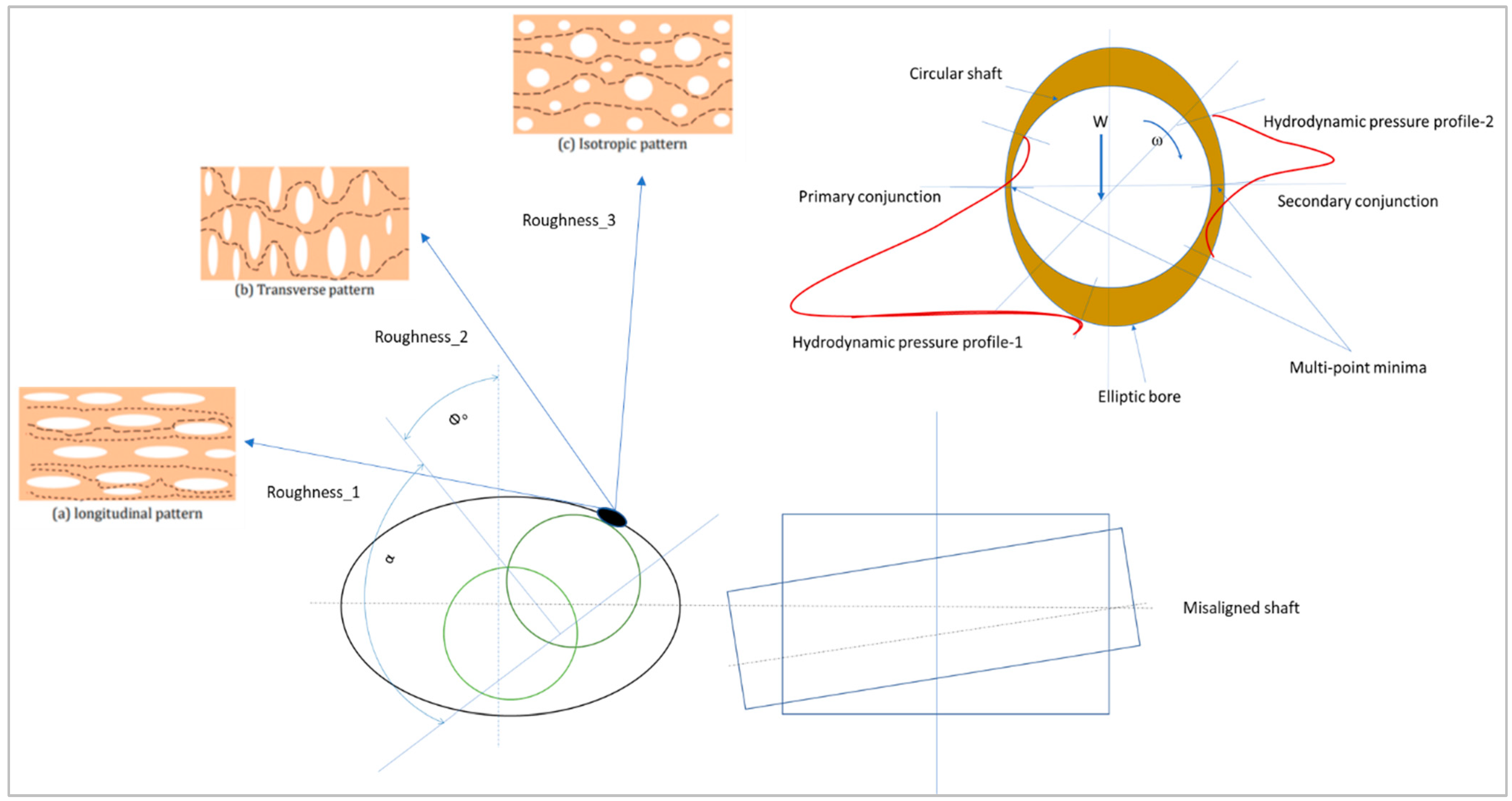
Film thickness is one of the primary parameters for bearing performance evaluation. Mishra [18] developed a film parameter for rough elliptic bore misaligned journal bearing, involving bore eccentricity(ε), ellipticity (G), misalignment (D_m), transverse, and longitudinal roughness [21] orientation (h_t, h_l). The instantaneous film profile of rough elliptic bore misaligned journal bearing in [16] is shown in Equation (1):

$$h_s=c\left\{\begin{array}{l}1+G{\cos }^2\left(\theta -\alpha \right)+{\in }_o\cos \left(\theta -{\varphi }_o\right)\\ +\psi {\tau }^{*}\cos \left(\theta -\alpha -{\varphi }_o\right)\end{array}\right\}-h_t+h_l$$

(1)

where

$$\psi =D_m{\psi }_{\max }$$

In addition,

$${\psi }_{\max }=2\left\{{\left(1-{\in }_o^2{\sin }^2\alpha \right)}^{\frac{1}{2}}-{\in }_o\cos \alpha \right\}$$

The model has a limitation of working within 0.1 < ε < 0.9, 0 < D_m < 0.9, 0 < G < 3.0. The roughness pattern in both transverse and longitudinal directions is assumed to be a sinusoidal wave with a roughness amplitude of 5 µm. The schematic of the misaligned rough elliptic bore journal bearing is shown in Figure 1. Table 1 shows the expectancy operators for the rough bearing.

$$h_t=A_t\sin \left(\frac{2\pi x}{\lambda t}\right)$$

In addition,

$$h_l=A_l\sin \left(\frac{2\pi x}{\lambda l}\right)$$

Figure 1. Misaligned rough elliptic bore journal bearing schematic.

Figure 1. Misaligned rough elliptic bore journal bearing schematic.

Table 1. Expectancy operator.

Film Terms	Value
$\xi \left(h\right)$	$1+G{\cos }^2\theta +\in \cos \theta$
$\xi \left(\frac{1}{h}\right)$	$\frac{35}{37y^7}\left\{6\left(y^2-h^2\right)\log \left(\frac{y+h}{y-h}\right)+\frac{2}{5}yh\left(15h^4-40y^2{h}^2+33y^4\right)\right\}$
$\xi \left(h^3\right)$	$h^3+\frac{h{y}^2}{3}$

Table 1. Expectancy operator.

Film Terms	Value
$\xi \left(h\right)$	$1+G{\cos }^2\theta +\in \cos \theta$
$\xi \left(\frac{1}{h}\right)$	$\frac{35}{37y^7}\left\{6\left(y^2-h^2\right)\log \left(\frac{y+h}{y-h}\right)+\frac{2}{5}yh\left(15h^4-40y^2{h}^2+33y^4\right)\right\}$
$\xi \left(h^3\right)$	$h^3+\frac{h{y}^2}{3}$

2.2. Thermohydrodynamics of Misaligned Rough Elliptic Bore Journal Bearing

Lubrication performance is quantitatively determined using the Reynolds equation [18]. Both hydrodynamic as well as elasto-hydrodynamic lubrication principles were developed mathematically to formulate and solve the film pressure by involving the film profile, lubricant rheology, shaft rotational speed, etc., as the input to these models [18]. The Reynolds equation is case-specific and involves modification based on geometry and operational requirements. Dien et al. [22] developed a time-dependent Careau viscosity model based on the modified Reynolds equation, as shown in Equation (2).

$$\frac{\partial }{\partial x}\left(\frac{\rho \xi \left(h^3\right)}{\eta }\frac{\partial p}{\partial x}\right)+\frac{\partial }{\partial z}\left(\frac{\rho \xi \left(h^3\right)}{{\mu }^{*}}\frac{\partial p}{\partial z}\right)=6\omega r_j\left(1-\frac{2}{\omega }\stackrel{*}{\mathsf{\Phi }}\right)+12\rho \stackrel{*}{e}\cos \left(\theta -\mathsf{\Phi }\right)$$

(2)

where

$$\lambda ={\mu }^{*}+2{\lambda }^2{\left(\frac{u_2-u_1}{\xi \left(h\right)}\right)}^2\left({\mu }_0-{\mu }_{\infty }\right)\left(\frac{n-1}{2}\right){\left(1+{\lambda }^2{\left(\frac{u_2-u_1}{\xi \left(h\right)}\right)}^2\right)}^{\frac{n-3}{2}}$$

In addition,

$${\mu }^{*}={\mu }_{\infty }+\left({\mu }_{\infty }-{\mu }_0\right){(1+{\lambda }^2\mathsf{\Gamma })}^{\frac{n-3}{2}}$$

Moreover,

$$\mathsf{\Gamma }=\frac{{\left(u_2-u_1\right)}^2+{\left(v_2-v_1\right)}^2}{\xi \left(h^2\right)}$$

Jamali and Al-Hammad [20] developed a dimensionless density (θ_c = ρ/ρ_cav) based on the Reynolds equation, which is capable of performance evaluation in both the full-fluid film and cavitation region [16], as shown in Equation (3).

$$\begin{array}{l}\frac{\partial }{\partial x}\left(\frac{{\rho }_c\xi \left(h^3\right)g{\beta }_b}{\eta }\frac{\partial {\theta }_c}{\partial x}\right)+\frac{\partial }{\partial z}\left(\frac{{\rho }_c\xi \left(h^3\right)g{\beta }_b}{{\mu }^{*}}\frac{\partial {\theta }_c}{\partial z}\right)\hspace{0.17em}\\ \hspace{0.17em}=\hspace{0.17em}\hspace{0.17em}\\ 6\omega r_j\left(1-\frac{2}{\omega }\stackrel{*}{\mathsf{\Phi }}\right)\frac{\partial {\rho }_c\xi \left(h\right){\theta }_c}{\partial x}+12{\rho }_c{\theta }_c\stackrel{*}{e}\cos \left(\theta -\mathsf{\Phi }\right)\end{array}$$

(3)

The finite difference method is used to solve these second-order partial differential equations. The boundary value problem involves mass-conserving boundary conditions. The method involves a switch function, g(θ_c), that plays an importance role in the cavitation index, where g(θ_c) = 1 for p ≥ p_cav and ρ ≥ ρ_cav, while g(θ_c) = 0 for p ≤ p_cav and ρ ≤ ρ_cav. In this Reynolds equation, the Poiseuille term is centrally discretized, while the Couette equation uses backward differentiation. The latter is more dominant in the cavitation region. The numerical technique involves the low-relaxation effective influence Newton-Raphson iterative method for pressure error convergence. In the zone of cavitation, the liquid mass content is controlled by ρ_cav, θ_c, and h (as ρ_cav.θ_c.h), where h is the film thickness. This variable is the dimensionless density, which is the fraction of lubricant content in the cavitation zone. Here, (1 − θ_c) is the cavity void fraction. When a solution to θ_c is obtained, the pressure profile can be reconstructed. The unwrapped bearing surface is discretized to form a grid of (94 × 16), which gives a square grid element for the stable hydrodynamic pressure [18] of film geometry. Film geometry plays an important role in the 3D hydrodynamic pressure profile. Misalignment reduces the longitudinal distribution of the pressure into a small area of bearing surface with a more concentrated pressure profile [18]. Due to non-circularity in terms of ellipticity, secondary pressure bumps with reduced peaks are formed. The roughness-induced pressure profile distorted from the smooth profile is due to many micro-scale lubricating conjunctions.

Rheology of the model. The hydrodynamic pressure in a contact conjunction was greatly affected due to an increase in the temperature of lubricant as a result of shear thinning. This thermally modified pressure can be estimated through viscosity-pressure-temperature interrelationship and density-pressure-temperature interrelationship, as shown by Roeland [23] and Dowson-Higginson [24]

$${\mu }^{*}={\mu }_0\exp \left(\ln {\mu }_0+9.67\right)\left(-1+{\left(1+5.1\times {10}^{-9}p\right)}^z\right)-\gamma \left(T-T_0\right)$$

(3a)

In addition,

$$\rho ={\rho }_0\left(1+\frac{0.6\times {10}^{-9}p}{1+1.7\times {10}^{-9}p}\right)\left(1-{\beta }_t\left(T-T_0\right)\right)$$

(3b)

2.3. Numerical Method for Film Temperature Evaluation

The intermediate lubricant layer moves rapidly and relatively, due to which fluid friction arises. This friction leads to a rise in temperature due to frictional heat generation [25]. The temperature distribution across the film depends largely on the fluid flow and rapid change in fluid geometry. Heat generation in the lubricating system is due to the heat of viscous shear and compression, whereas heat generation out of the system is due to cooling by convection across the oil film and by conduction through the shaft and sleeve. In Equation (4), the energy equation using the Carreau viscosity model [18] is shown, which is a partial differential equation involving film pressure and temperature as variables. It can be solved by the finite difference method, with a known initial value of pressure and a boundary value of temperature.

$$\begin{array}{l}\left\{\left(\rho c_f\frac{u_2}{2}\xi \left(h\right)-\rho c_f\frac{\xi \left(h^3\right)}{12\eta }\frac{\partial p}{\partial x}\right)\frac{\partial T_m}{\partial x}-\left(\rho c_f\frac{\xi \left(h^3\right)}{12{\mu }^{*}}\frac{\partial p}{\partial z}\right)\frac{\partial T_m}{\partial z}\right\}\\ =\\ \left\{\begin{array}{l}{\mu }^{*}\left(\frac{u_2{}^2}{\xi \left(h\right)}\right)+\left({\beta }_t\xi \left(h\right)T_m\frac{u_2}{2}\right)\frac{\partial p}{\partial x}+\left(\frac{\xi \left(h^3\right)}{12\eta }-{\beta }_t{T}_m\frac{\xi \left(h^3\right)}{12\eta }\right){\left(\frac{\partial p}{\partial x}\right)}^2\\ +\left(\frac{\xi \left(h^3\right)}{12{\mu }^{*}}-{\beta }_t{T}_m\frac{\xi \left(h^3\right)}{12{\mu }^{*}}\right){\left(\frac{\partial p}{\partial z}\right)}^2+{\beta }_t\xi \left(h\right)T_m\frac{\partial p}{\partial T}-\rho c_f\xi \left(h\right)\frac{\partial T_m}{\partial t}\end{array}\right\}\end{array}$$

(4)

The mean temperature is derived from Equation (4) and shown as Equation (5).

$$T_m=\frac{\left\{\begin{array}{l}\left(\rho c_f\frac{u_2}{2}\xi \left(h\right)-\rho c_f\frac{\xi \left(h^3\right)}{12\eta }\frac{\partial p}{\partial x}\right)\frac{\partial T_m}{\partial x}-\left(\rho c_f\frac{\xi \left(h^3\right)}{12{\mu }^{*}}\frac{\partial p}{\partial z}\right)\frac{\partial T_m}{\partial z}-\\ {\mu }^{*}\left(\frac{u_2{}^2}{\xi \left(h\right)}\right)-\hspace{0.17em}\frac{\xi \left(h^3\right)}{12\eta }{\left(\frac{\partial p}{\partial x}\right)}^2-\frac{\xi \left(h^3\right)}{12{\mu }^{*}}{\left(\frac{\partial p}{\partial z}\right)}^2-\rho c_f\xi \left(h\right)\left(\frac{\partial T_m}{\partial t}\right)\end{array}\right\}}{\left({\beta }_t\xi \left(h\right)T_m\frac{u_2}{2}\right)\frac{\partial p}{\partial x}-{\beta }_t\frac{\xi \left(h^3\right)}{12\eta }{\left(\frac{\partial p}{\partial x}\right)}^2-{\beta }_t\frac{\xi \left(h^3\right)}{12{\mu }^{*}}{\left(\frac{\partial p}{\partial z}\right)}^2+{\beta }_t\left(\frac{\partial p}{\partial t}\right)}$$

(5)

The solution of the abovementioned equation of temperature uses the finite difference method to discretize the right-hand side with the central differentiation technique [26]. The low-relaxation iterative algorithm is used for temperature error convergence. The generated conjunction heat is dissipated to the rotating journal and stationary sleeve. It is assumed that the heat of convection through the fluid film in the flow direction (along circumference) is significantly less compared to the side leakage direction (along the bearing length). The temperature at the first node is considered ambient, which indicates that T (0, z) = T_o. The temperature at the inlet is equal to the temperature at the outlet along the length of the bearing, which indicates that T (θ, z) = T (θ, −z).

Table 2. Model input parameters.

Input Variables	Values	Input Variables	Values
Shaft radius, (rj)	0.025 m	Characteristic relaxation	4.0 × 10−6
Bearing length, (L)	0.030 m	Time constant, (λ)	3.0 × 10−6
Radial clearance, (c)	60 µm	Lubricant density, (ρ)	860 kg/m3
Rotational speed, (N)	7000 rpm	Lubricant specific heat, (Cf)	1950 J/kgK
Wavelength of roughness, (γl/γt)	0.005 m	Inlet lubricant temperature, (To)	315 K
Lubricant details		Viscosity pressure index, (Z)	0.65
Lubricant type	SAE10W50	Temperature coefficient of viscosity, (γ)	0.0310225 K−1
Limiting viscosity at low shear rate (µ0)	0.105 PaS	Coefficient of thermal expansion, (βt)	0.000792 K−1
Limiting viscosity at high shear rate (µ∞)	0.055 PaS

shows the model input parameters required for the simulation. The bearing considered for analysis is a self-aligning journal bearing with bearing code of SA 35M/S4170, which is lubricated with an oil ring and has a maximum load capacity of 10 kN.

The load carrying capacity of the bearing is estimated by integrating the hydrodynamic pressure over the area of conjunction. The resolved component of this reactive force is shown as:

$$F_x=-{\displaystyle \underset{0}{\overset{L}{\mathsf{\int }}}{\displaystyle \underset{0}{\overset{\theta }{\mathsf{\int }}}\left(pr\cos \theta \right)}}d\theta dz$$

(6)

$$F_y=-{\displaystyle \underset{0}{\overset{L}{\mathsf{\int }}}{\displaystyle \underset{0}{\overset{\theta }{\mathsf{\int }}}\left(pr\sin \theta \right)}}d\theta dz$$

(7)

Furthermore, the hydrodynamic action can be resolved in radial and circumferential directions as follows:

$$F_r=-F_x\cos \varphi -F_z\sin \varphi$$

(8)

$$F_{\varphi }=-F_x\sin \varphi -F_z\cos \varphi$$

(9)

The resultant bearing load and attitude angle is shown as:

$$W={\left(F_r{}^2+F_{\varphi }{}^2\right)}^{\frac{1}{2}}$$

(10)

$$\varphi ={\tan }^{-1}\left(-\frac{F_{\varphi }}{F_r}\right)$$

(11)

Linearization of bearing equation [27] is shown as:

$$\frac{1}{r_j{}^2}\frac{\partial }{\partial \theta }\left(\frac{\rho \xi \left(h_s{}^3\right)}{12\eta }\frac{\partial p_s}{\partial \theta }\right)+\frac{\partial }{\partial z}\left(\frac{\rho \xi \left(h_s{}^3\right)}{12{\mu }^{*}}\frac{\partial p_s}{\partial z}\right)=\frac{U}{2r_j}\frac{\partial \rho \xi \left(h_s\right)}{\partial \theta }$$

(12)

Or

$$\begin{array}{l}\frac{1}{r_j{}^2}\frac{\partial }{\partial \theta }\left(\frac{\rho \xi \left(h_s{}^3\right)}{12\eta }\frac{\partial p_x}{\partial \theta }\right)+\frac{\partial }{\partial z}\left(\frac{\rho \xi \left(h_s{}^3\right)}{12{\mu }^{*}}\frac{\partial p_x}{\partial z}\right)\\ =\\ \frac{U}{2r_j}\frac{\partial \left(\rho \cos \theta \right)}{\partial \theta }-\frac{1}{r_j{}^2}\frac{\partial }{\partial \theta }\left(\frac{\rho \xi \left(h_s{}^2\right)\cos \theta }{4\eta }\frac{\partial p_s}{\partial \theta }\right)\\ -\frac{\partial }{\partial z}\left(\frac{\rho \xi \left(h_s{}^2\right)\cos \theta }{4{\mu }^{*}}\frac{\partial p_s}{\partial z}\right)\end{array}$$

(13)

Therefore,

$$\frac{1}{r_j{}^2}\frac{\partial }{\partial \theta }\left(\frac{\rho \xi \left(h_s{}^3\right)}{12\eta }\frac{\partial p_{x*}}{\partial \theta }\right)+\frac{\partial }{\partial z}\left(\frac{\rho \xi \left(h_s{}^3\right)}{12{\mu }^{*}}\frac{\partial p_{x*}}{\partial z}\right)=\rho \cos \theta$$

(14)

In addition,

$$\frac{1}{r_j{}^2}\frac{\partial }{\partial \theta }\left(\frac{\rho \xi \left(h_s{}^3\right)}{12\eta }\frac{\partial p_{z*}}{\partial \theta }\right)+\frac{\partial }{\partial z}\left(\frac{\rho \xi \left(h_s{}^3\right)}{12{\mu }^{*}}\frac{\partial p_{z*}}{\partial z}\right)=\rho \sin \theta$$

(15)

The dimensionless spring and damping coefficients are shown as:

$$\left(\begin{array}{cc}{K}_{xx}& K_{xz}\\ K_{zx}& K_{zz}\end{array}\right)=-\frac{c}{W}\left(\begin{array}{cc}{\displaystyle \underset{0}{\overset{L}{\mathsf{\int }}}{\displaystyle \underset{0}{\overset{2\pi }{\mathsf{\int }}}{p}_x{r}_j\cos \theta d\theta dz}}& {\displaystyle \underset{0}{\overset{L}{\mathsf{\int }}}{\displaystyle \underset{0}{\overset{2\pi }{\mathsf{\int }}}{p}_z{r}_j\cos \theta d\theta dz}}\\ {\displaystyle \underset{0}{\overset{L}{\mathsf{\int }}}{\displaystyle \underset{0}{\overset{2\pi }{\mathsf{\int }}}{p}_x{r}_j\sin \theta d\theta dz}}& {\displaystyle \underset{0}{\overset{L}{\mathsf{\int }}}{\displaystyle \underset{0}{\overset{2\pi }{\mathsf{\int }}}{p}_z{r}_j\sin \theta d\theta dz}}\end{array}\right)$$

(16)

$$\left(\begin{array}{cc}{B}_{xx}& B_{xz}\\ B_{zx}& B_{zz}\end{array}\right)=-\frac{c\omega }{W}\left(\begin{array}{cc}{\displaystyle \underset{0}{\overset{L}{\mathsf{\int }}}{\displaystyle \underset{0}{\overset{2\pi }{\mathsf{\int }}}{p}_{x*}{r}_j\cos \theta d\theta dz}}& {\displaystyle \underset{0}{\overset{L}{\mathsf{\int }}}{\displaystyle \underset{0}{\overset{2\pi }{\mathsf{\int }}}{p}_{y*}{r}_j\cos \theta d\theta dz}}\\ {\displaystyle \underset{0}{\overset{L}{\mathsf{\int }}}{\displaystyle \underset{0}{\overset{2\pi }{\mathsf{\int }}}{p}_{x*}{r}_j\sin \theta d\theta dz}}& {\displaystyle \underset{0}{\overset{L}{\mathsf{\int }}}{\displaystyle \underset{0}{\overset{2\pi }{\mathsf{\int }}}{p}_{y*}{r}_j\sin \theta d\theta dz}}\end{array}\right)$$

(17)

$${\mathsf{\Omega }}^2{M}_{CR}=\frac{B_{xx}{K}_{zz}+B_{zz}{K}_{xx}-B_{zx}{K}_{xz}-B_{xz}{K}_{zx}}{B_{xx}+B_{zz}}$$

(18)

$${\mathsf{\Omega }}^2=\frac{\left(K_{xx}-{\mathsf{\Omega }}^2{M}_{CR}\right)\left(K_{zz}-{\mathsf{\Omega }}^2{M}_{CR}\right)-K_{xz}{K}_{zx}}{B_{xx}{B}_{zz}-B_{xz}-B_{zx}}$$

(19)

2.4. Method for Grey-Fuzzy Hybrid Optimization Model of Rough Elliptic Bore Misaligned Journal Bearing

The present work utilized integrated algorithms of grey relational analysis and fuzzy logic to optimize the various responses. The process outline of this hybrid optimization is represented through a flowchart and is shown in Figure 2.

In the grey theory, the term grey denotes the primitive data with deprived, incomplete, and unclear information. Moreover, it provides the incomplete connection of information among these data. Grey relational analysis (GRA) utilizes the quantitative exploration to define the degree of relationship among experimentally obtained results and a target value in the grey system. The extent of relationship among these sequences can be expressed as the grey relational coefficient. In the grey relational analysis, the raw data of W_is, W_th, F_is, F_th, Q_is, and Q_th are initially normalized in the range between 0 and 1 (four avoiding the unit of responses) and this process is known as the grey relational generation. For normalization, the responses, such as W_is, W_th, Q_is, and Q_th have followed the larger-the-better characteristics (Equation (20)), while the other responses (F_is and F_th) have followed the smaller-the-better characteristics (Equation (21)).

$$X_i(x)=\frac{Z_i(x)-\min Z_i(x)}{\max Z_i(x)-\min Z_i(x)}$$

(20)

$$X_i(x)=\frac{\max Z_i(x)-Z_i(x)}{\max Z_i(x)-\min Z_i(x)}$$

(21)

where ‘X_i (x)’ is the normalized data of ith experiment for xth response, Z is the response data, ‘i’ symbolizes the number of experiments, i.e., i = 1, 2, 3, …, 27, ‘x’ is the number of response, i.e., x =1, 2, 3, …, 6, and ‘min Z_i(x)’ and ‘max Z_i(x)’ are the least and largest value of ‘Z_i(x)’ for xth response, respectively.

Furthermore, considering normalized data, the grey relational coefficient (GRC) for each response is evaluated using Equation (22).

$$C_i(x)=\frac{K_{\min }+\lambda K_{\max }}{K_{0i}(x)+\lambda K_{\max }}$$

(22)

where $K_{0i}(x)=\Vert {\epsilon }_0(x)-{\epsilon }_i(x)\Vert$ is the absolute value of difference between the $K_0(x)$ and $K_i(x)$, $K_{\min }$ and $K_{\max }$ are the least and largest value of $K_{0i}(x)$ independently, and ‘λ’ is a distinguishing term which lies between 0 and 1. In the current work, ‘λ’ is considered as 0.5.

Furthermore, the grey relational grade (GRG) is a single response data that is estimated using Equation (23).

$$G_i=\frac{1}{m}{\displaystyle \sum _{x=1}^m{\lambda }_i(x)}$$

(23)

where ‘G_i’ is the grey relational grade for ith experiment and m denotes the number of response characteristics.

The fuzzy logical system is an artificial intelligence technique that can deal with uncertainty and anticipate future outcomes [28]. The fuzzy model comprises the fuzzifier, modem’s membership relations, rule inference (as shown in Figure 3), inference engine, and de-fuzzifier. Initially, the fuzzifier applies the modem’s membership relations to fuzzify the grey relational coefficients (GRC). The membership function (MF) defines the mapping of inputs and outputs. Several types of MF, such as Trapezoidal, Sigmoidal, Gaussian, and Triangular have been found in the literature. Among these types, Gaussian membership function is the most popular due to several advantageous features, such as local although not stringently compact, exhibiting a very smooth output, and predictions that are non-probabilistic [12]. Therefore, Gaussian membership function is utilized here to achieve the grey-fuzzy grade (GFG) value. Seven numbers of MF (VVL—very very low, VL—very low, L—low, M—medium, H—high, VH—very high, and VVH—very very high) are considered for each input and output. Moreover, the membership graph for each input and output is displayed in Figure 4 and Figure 5, respectively. Furthermore, 20 different fuzzy rules are utilized to achieve the predicted data of GFG. To de-fuzzify the output data, most of the prevailing centroid technique is utilized to achieve more crispy output results [29]. The fuzzy rules viewer is utilized to achieve the GFG data for all the experimental runs. All these activities for predicting GFG are accomplished using the ‘fuzzy’ tool available in Matlab-R2013a software from MathWorks.

3. Results and Discussion

3.1. Rough Elliptic Bore Misaligned Journal Bearing Static Performance Analysis

Due to the presence of geometrical abnormalities, the film profile varies accordingly. In the case of an elliptic bore, two conjunctions (converging diverging zones) exist with two minima, which are symmetrically located with respect to the mean position, as compared to the single point minima in the case of circular bore [16]. Furthermore, a circular bore with misalignment bears a single point of minima in arbitrary positions, while the induction of roughness creates micro-conjunctions of 0.2 µm in amplitude.

The film thickness and hydrodynamic pressure profile in three-dimensional form is shown in Figure 6a,b, respectively. In Equation (3), the hydrodynamic pressure is more evenly distributed in the case of an elliptic bore bearing without misalignment compared with misalignment. In the former case, there is a 20% increase in pressure spike, whereas in the case of a circular misaligned case, there is a concentrated pressure which may lead to a metal-to-metal contactor with a higher degree of instability. The rough elliptic bore misaligned journal bearing configuration provides a more distributed pressure profile compared with the misaligned smooth elliptic bore, although the peak hydrodynamic pressure is reduced to 33%. However, the bearing stability is better in the former case.

The rapid shear of the lubricant layer develops a temperature in the film. Therefore, the developed heat was transferred across the film to the rotating shaft and stationary bore through the conduction mode. The viscosity and density dependence of temperature is shown in Equation (3a,b). For G = 1.0, ε = 0.6, and D_m = 0, the isotherms are regular with an 8 °C difference in temperature. Figure 7a,b shows the temperature contour of bearing surface for the longitudinal and transverse pattern of roughness, respectively, with the highest temperature as 47 °C. At the angular location of minimum film thickness, with a degree of misalignment of D_m = 0.8, the trend of the isotherm changed (moved to a different location) and the maximum temperature was reduced to 43 °C in the corresponding region. Reduction in temperature is due to turbulence in the conjunction as a result of rough-elliptic-misaligned geometry. The presence of transverse/longitudinal roughness leads to a variation in higher order isotherms and their contour profile on the bearing surface. Although no significant profile variation on lower order isotherms exists, the misaligned rough elliptic bore journal bearing has dynamic characteristics.

With the increasing eccentricity ratio, K_xx decreases by 62% between 0.3 < and < 0.9. For a particular eccentricity in this range, the K_xx is higher for a higher degree of misalignment, with is a 68% increase in K_xx for ΔD_m = 0.9. The power index (PI) has little or no effect on K_xx. However, for a higher degree of misalignment, the K_xx is higher for any PI. The highest value of K_xx of 0.61 occurs at a PI of 0.6 and D_m = 0.0. Similarly, the angular speed has little or no effect on K_xx. The maximum K_xx is 0.61 at 3000 rpm for 0.9 degrees of misalignment (D_m). At particular G, K_xx increases with the increase in D_m. For ΔD_m = 0.9, a 76.4% increase in K_xx is observed. The increment follows a parabolic trend, with K_xx having a lower value at the higher value of G.

The K_xz and K_zx have a reversing trend. The K_xz increases with an increasing eccentricity ratio; (dK_xz/dε) = 0.45 for D_m = 0; (dK_xz/dε) = 0.56 for D_m = 0.5; and (dK_xz/dε) = 0.63 for Dm = 0.9. Similar to K_xx, K_xz has negligible change with an increase in PI and angular speed (N) of the shaft. At particular PI, (K_xz)_Dm=0 > (K_xz)_Dm=0.5 > (K_xz)_Dm=0.9. The K_xz response to D_m follows a parabolic trend with various ellipticities (G). For a particular non-circularity, K_xz increases with the increasing D_m. At a certain degree of misalignment (D_m), K_xz is higher for higher non-circularity. Details of all dynamic stability parameters are shown in Table 3, Table 4, Table 5 and Table 6. Variations of K_xx, K_xz, K_zx, K_zz, B_xx, B_xz, B_zx, B_zz, M_cr, and Ω for various combinations of (ε,D_m), (PI,D_m), (N,D_m), and (G,D_m) are stated in these tables.

Figure 6. Misaligned rough elliptic bore journal bearing. (a) Three-dimensional film profile [18]; (b) three-dimensional pressure profile [18].

Figure 6. Misaligned rough elliptic bore journal bearing. (a) Three-dimensional film profile [18]; (b) three-dimensional pressure profile [18].

Figure 7. Misaligned rough elliptic bore journal bearing temperature counter. (a) Longitudinal pattern [18]; (b) transverse pattern [18].

Figure 7. Misaligned rough elliptic bore journal bearing temperature counter. (a) Longitudinal pattern [18]; (b) transverse pattern [18].

Table 3. Combined eccentricity and misalignment effect on stability parameters.

	Kxx	Kxz	Kzx	Kzz	Bxx	Bxz	Bzx	Bzz	Mcr	Ω
ε (0.3), Dm (0)	0.45	−1.1	3.2	1.5	5.0	−2.4	−4.8	2.8	3.3	0.145
ε (0.3), Dm (0.5)	0.33	−0.8	5.1	2.4	8.5	−3.7	−7.6	4.5	5.3	0.145
ε (0.3), Dm (0.9)	0.22	−0.45	5.4	2.6	9.1	−4.0	−8.1	5.0	5.6	0.145
ε (0.6), Dm (0)	0.75	−0.9	2.1	1.0	3.0	−1.7	−3.3	1.9	2.3	0.145
ε (0.6), Dm (0.5)	0.55	−1.25	3.6	1.7	5.6	−2.6	−5.2	3.2	3.7	0.145
ε (0.6), Dm (0.9)	0.21	−0.78	3.8	1.9	6.0	−2.9	−5.7	3.4	3.9	0.145
ε (0.9), Dm (0)	0.8	−1.95	1.2	0.6	1.3	−1.0	−1.9	1.0	1.4	0.145
ε (0.9), Dm (0.5)	0.45	−1.35	1.9	1.0	2.8	−1.6	−3.2	1.8	2.2	0.145
ε (0.9), Dm (0.9)	0.33	−0.85	2.1	1.2	2.97	−1.8	−3.5	1.9	2.35	0.145

Table 3. Combined eccentricity and misalignment effect on stability parameters.

	Kxx	Kxz	Kzx	Kzz	Bxx	Bxz	Bzx	Bzz	Mcr	Ω
ε (0.3), Dm (0)	0.45	−1.1	3.2	1.5	5.0	−2.4	−4.8	2.8	3.3	0.145
ε (0.3), Dm (0.5)	0.33	−0.8	5.1	2.4	8.5	−3.7	−7.6	4.5	5.3	0.145
ε (0.3), Dm (0.9)	0.22	−0.45	5.4	2.6	9.1	−4.0	−8.1	5.0	5.6	0.145
ε (0.6), Dm (0)	0.75	−0.9	2.1	1.0	3.0	−1.7	−3.3	1.9	2.3	0.145
ε (0.6), Dm (0.5)	0.55	−1.25	3.6	1.7	5.6	−2.6	−5.2	3.2	3.7	0.145
ε (0.6), Dm (0.9)	0.21	−0.78	3.8	1.9	6.0	−2.9	−5.7	3.4	3.9	0.145
ε (0.9), Dm (0)	0.8	−1.95	1.2	0.6	1.3	−1.0	−1.9	1.0	1.4	0.145
ε (0.9), Dm (0.5)	0.45	−1.35	1.9	1.0	2.8	−1.6	−3.2	1.8	2.2	0.145
ε (0.9), Dm (0.9)	0.33	−0.85	2.1	1.2	2.97	−1.8	−3.5	1.9	2.35	0.145

Table 4. Power index and misalignment effect on stability parameters.

	Kxx	Kxz	Kzx	Kzz	Bxx	Bxz	Bzx	Bzz	Mcr	Ω
PI (0.2), Dm (0)	0.36	−0.89	0.25	1.2	4.65	−1.8	−3.6	4.1	44	0.148
PI (0.2), Dm (0.5)	0.35	−1.25	0.41	2.0	7.54	−2.7	−5.8	3.8	41	0.148
PI (0.2), Dm (0.9)	0.34	−1.48	0.44	2.25	7.98	−2.48	−6.5	2.5	27.0	0.148
PI (0.34), Dm (0)	0.56	−0.9	0.23	1.1	4.8	−1.7	−3.8	4.0	45	0.148
PI (0.34), Dm (0.5)	0.55	−1.32	0.40	1.98	7.6	−2.74	−6.1	3.7	42	0.148
PI (0.34), Dm (0.9)	0.52	−1.4	0.45	2.05	8.1	−2.5	−6.6	2.4	26.3	0.148
PI (0.6), Dm (0)	0.61	−0.92	0.27	1.15	4.91	−1.8	−3.9	3.9	47	0.148
PI (0.6), Dm (0.5)	0.60	−1.50	0.43	1.96	7.63	−2.8	−6.2	3.6	42.5	0.148
PI (0.6), Dm (0.9)	0.58	−1.52	0.47	2.14	8.25	−2.6	−6.7	2.3	27.3	0.148

Table 4. Power index and misalignment effect on stability parameters.

	Kxx	Kxz	Kzx	Kzz	Bxx	Bxz	Bzx	Bzz	Mcr	Ω
PI (0.2), Dm (0)	0.36	−0.89	0.25	1.2	4.65	−1.8	−3.6	4.1	44	0.148
PI (0.2), Dm (0.5)	0.35	−1.25	0.41	2.0	7.54	−2.7	−5.8	3.8	41	0.148
PI (0.2), Dm (0.9)	0.34	−1.48	0.44	2.25	7.98	−2.48	−6.5	2.5	27.0	0.148
PI (0.34), Dm (0)	0.56	−0.9	0.23	1.1	4.8	−1.7	−3.8	4.0	45	0.148
PI (0.34), Dm (0.5)	0.55	−1.32	0.40	1.98	7.6	−2.74	−6.1	3.7	42	0.148
PI (0.34), Dm (0.9)	0.52	−1.4	0.45	2.05	8.1	−2.5	−6.6	2.4	26.3	0.148
PI (0.6), Dm (0)	0.61	−0.92	0.27	1.15	4.91	−1.8	−3.9	3.9	47	0.148
PI (0.6), Dm (0.5)	0.60	−1.50	0.43	1.96	7.63	−2.8	−6.2	3.6	42.5	0.148
PI (0.6), Dm (0.9)	0.58	−1.52	0.47	2.14	8.25	−2.6	−6.7	2.3	27.3	0.148

Table 5. Combined angular speed and misalignment effect on stability parameters.

	Kxx	Kxz	Kzx	Kzz	Bxx	Bxz	Bzx	Bzz	Mcr	Ω
N (3000), Dm (0)	0.33	−8.4	0.22	1.20	1.4	−0.7	−1.4	0.8	6	4.4
N (3000), Dm (0.5)	0.30	−13.65	0.35	1.85	2.3	−0.95	−1.9	1.3	5.2	4.4
N (3000), Dm (0.9)	0.29	−14.68	0.41	2.0	2.6	−1.1	−2.2	1.4	5.0	4.4
N (6000), Dm (0)	0.53	−8.7	0.25	1.25	3.1	−1.2	−2.7	1.6	11.0	2.2
N (6000), Dm (0.5)	0.51	−13.7	0.4	1.95	4.8	−1.95	−4.0	2.5	18.0	2.2
N (6000), Dm (0.9)	0.49	−14.7	0.43	2.12	5.2	−2.2	−4.7	2.7	20.0	2.2
N (9000), Dm (0)	0.62	−8.8	0.2	1.32	4.5	−1.7	−4.0	2.4	25.0	1.5
N (9000), Dm (0.5)	0.59	−13.72	0.34	1.98	7.3	−3.0	−6.1	3.7	41.0	1.5
N (9000), Dm (0.9)	0.57	−14.73	0.44	2.31	7.8	−3.2	−6.3	4.1	45.0	1.5

Table 5. Combined angular speed and misalignment effect on stability parameters.

	Kxx	Kxz	Kzx	Kzz	Bxx	Bxz	Bzx	Bzz	Mcr	Ω
N (3000), Dm (0)	0.33	−8.4	0.22	1.20	1.4	−0.7	−1.4	0.8	6	4.4
N (3000), Dm (0.5)	0.30	−13.65	0.35	1.85	2.3	−0.95	−1.9	1.3	5.2	4.4
N (3000), Dm (0.9)	0.29	−14.68	0.41	2.0	2.6	−1.1	−2.2	1.4	5.0	4.4
N (6000), Dm (0)	0.53	−8.7	0.25	1.25	3.1	−1.2	−2.7	1.6	11.0	2.2
N (6000), Dm (0.5)	0.51	−13.7	0.4	1.95	4.8	−1.95	−4.0	2.5	18.0	2.2
N (6000), Dm (0.9)	0.49	−14.7	0.43	2.12	5.2	−2.2	−4.7	2.7	20.0	2.2
N (9000), Dm (0)	0.62	−8.8	0.2	1.32	4.5	−1.7	−4.0	2.4	25.0	1.5
N (9000), Dm (0.5)	0.59	−13.72	0.34	1.98	7.3	−3.0	−6.1	3.7	41.0	1.5
N (9000), Dm (0.9)	0.57	−14.73	0.44	2.31	7.8	−3.2	−6.3	4.1	45.0	1.5

Table 6. Combined non-circularity and misalignment effect on stability parameters.

	Kxx	Kxz	Kzx	Kzz	Bxx	Bxz	Bzx	Bzz	Mcr	Ω
G (1.0), Dm (0)	0.18	−0.5	0.97	3.3	2.0	−0.8	−1.8	5.9	45	0.215
G (1.0), Dm (0.5)	0.26	−0.0.7	1.04	5.0	2.3	−0.9	−2.0	6.4	49	0.215
G (1.0), Dm (0.9)	0.28	−0.78	1.08	5.3	2.4	−1.2	−2.2	6.6	50	0.215
G (2.0), Dm (0)	0.36	−0.95	0.36	1.0	4.5	−1.8	−3.7	2.3	17	0.215
G (2.0), Dm (0.5)	0.58	−1.5	0.41	1.7	5.0	−1.9	−4.1	2.5	19	0.215
G (2.0), Dm (0.9)	0.6	−1.57	0.44	2.1	5.2	−2.0	−4.3	2.7	20	0.215
G (3.0), Dm (0)	0.98	−2.5	0.12	0.6	12.0	−4.8	−9.7	1.1	8	0.215
G (3.0), Dm (0.5)	1.46	−3.6	0.19	1.1	12.7	−4.9	−10.3	1.3	9	0.215
G (3.0), Dm (0.9)	1.5	−3.8	0.21	1.34	13.2	−5.1	−10.6	1.4	10	0.215

Table 6. Combined non-circularity and misalignment effect on stability parameters.

	Kxx	Kxz	Kzx	Kzz	Bxx	Bxz	Bzx	Bzz	Mcr	Ω
G (1.0), Dm (0)	0.18	−0.5	0.97	3.3	2.0	−0.8	−1.8	5.9	45	0.215
G (1.0), Dm (0.5)	0.26	−0.0.7	1.04	5.0	2.3	−0.9	−2.0	6.4	49	0.215
G (1.0), Dm (0.9)	0.28	−0.78	1.08	5.3	2.4	−1.2	−2.2	6.6	50	0.215
G (2.0), Dm (0)	0.36	−0.95	0.36	1.0	4.5	−1.8	−3.7	2.3	17	0.215
G (2.0), Dm (0.5)	0.58	−1.5	0.41	1.7	5.0	−1.9	−4.1	2.5	19	0.215
G (2.0), Dm (0.9)	0.6	−1.57	0.44	2.1	5.2	−2.0	−4.3	2.7	20	0.215
G (3.0), Dm (0)	0.98	−2.5	0.12	0.6	12.0	−4.8	−9.7	1.1	8	0.215
G (3.0), Dm (0.5)	1.46	−3.6	0.19	1.1	12.7	−4.9	−10.3	1.3	9	0.215
G (3.0), Dm (0.9)	1.5	−3.8	0.21	1.34	13.2	−5.1	−10.6	1.4	10	0.215

The bearing stiffness coefficient along the z-z direction (K_zz) increases with an increase in misalignment. At ε_0.3 for ΔD_m0.9, a 73% increase in K_zz is observed. Similarly, at ε_0.6, it is increased by 90% due to the degree of misalignment of ΔD_m0.9. It increases further at ɛ_0.9 for ΔD_m0.9 and is found to be 100%. Due to the combined effect of PI and misalignment, K_zz increases with the increasing value of D_m at particular PI_0.2/0.34/0.6. For PI_0.2 and ΔD_m0.9, the increase in K_zz is observed to be 89.6%. Similarly, for PI_0.34 and ΔD_m0.9, an 86.3% increase in K_zz is observed. At the highest power index (PI_0.9) and ΔD_m0.9, K_zz increases by 86.1%. At the highest D_m0.9, for ΔP_0.2–0.34, K_zz decreases by 10.3%_.

The combined effect of angular speed and misalignment shows that for ΔN_3000–9000, K_zz increases by 10%. For aligned bearing (D_m0.0) at 3000 rpm due to the first 50% increase in misalignment (ΔD_m0.0–0.5), K_zz increases by 66.7%. At this angular speed, which is further due to ΔD_m0.5–0.9, the K_zz increases by 8.1%. Similarly, at 6000 rpm, K_zz increases by 56% for a misalignment difference of ΔD_m0.0–0.5. Once again, for ΔD_m0.5–0.9, an 8.7% increase in K_zz is observed for the same angular speed. At 9000 rpm, the lower-level change in misalignment ΔD_m0.0–0.5, induces 50% more K_zz, whereas in the upper-level change in misalignment ΔD_m0.5–0.9, it increases by 16.7%. At a particular degree of misalignment, D_m0/0.5/0.9, K_zz increases with the increasing angular speed. At D_m0, for ΔN_3000–6000 and ΔN_6000–9000, an increase in K_zz is observed to be 4.17% and 5.6%, respectively. For an aligned bearing (D_m0.0), K_zz decreases with an increase in non-circularity range, ΔG_1.0–2.0, and ΔG_2.0–3.0, at a rate of 60% and 40%, respectively.

The misaligned cases exhibit a similar trend to the aligned cases. For G_1.0, at ΔD_m0.0–0.5, K_zz increases by 34%, whereas it increases by 6% for ΔD_m0.5.0–0.9 misalignment increment. For G_2.0, at ΔD_m0.0–0.5 and ΔD_m0.5–0.9, K_zz is observed to increase by 70% and 23.5%, respectively. For higher non-circularity G_3.0 and lower-level increment of ΔD_m0.0–0.5, K_zz is observed to increase by 83.3%, whereas for higher-level increment of ΔD_m0.5–0.9, it increases by 21.8%. The combination of lower non-circularity and misalignment elevates K_zz, while the higher non-circularity and misalignment has a diminishing effect on K_zz. There are four damping coefficients (B_xx, B_xz, B_zx, B_zz) associated with the bearing stability analysis, among which B_xx and B_zz are considered positive, while B_xz and B_zx are considered negative. The highest value of B_xx is 13.2 at G_3.0 and D_m0.9, whereas the lowest is 1.4 at N₃₀₀₀ and D_m0.0. At a particular eccentricity ratio (ε_0.3/0.6/0.9), B_xx increases with the increasing misalignment. At lower eccentricity, ε_0.3, for ΔD_m0.0–0.5, B_xx is observed to increase by 70%, while for the same eccentricity and upper misalignment range, ΔD_m0.5–0.9, a 7% increase in B_xx is observed. At medium eccentricity, ε_0.6, a 7.1% increase in B_xx is observed for ΔD_m0.0–0.5 and ΔD_m0.5–0.9, respectively. At higher eccentricity, ɛ_0.9, B_xx growth is lowest. The rate of growth is 115% and 6%, respectively for the misalignment range of ΔD_m0.0–0.5 and ΔD_m0.5–0.9.

For aligned shafts, D_m0.0, B_xx decreases slightly for a range of PI_{0.2–0.34–0.6}. At a particular PI_0.2/0.34/0.6, for a lower range of misalignment ΔD_m0.0–0.5, B_xx is observed to increase by 62.1%, 58.4%, and 55.4% for the respective power index. Meanwhile, for higher misalignment range ΔD_m0.5–0.9, B_xx is observed to increase by 5.8%, 6.5%, and 8.1%. B_xx increases with the combined effect of angular speed and misalignment. The lowest is 1.4 at N₃₀₀₀ and D_m0.0, whereas the highest is 7.8 at N₉₀₀₀ and D_m0.9. B_xx increases with the combined effect of non-circularity (G_{1.0–2.0–3.0}) and misalignment (D_{m0.0–0.5–0.9}). The lowest is 2.0 at G_1.0 and D_m0.0, whereas the highest is 13.2 at G_3.0 and D_m0.9.

The damping coefficients, B_xz and B_zx, have a negative trend and increase with the combined effect of angular speed and misalignment, the lowest being −0.7 and −1.4, respectively, at 3000 rpm at D_m0.0 and the highest being −3.2 and −6.3, respectively. The next important damping coefficient is B_zz, acting in the z-z direction. B_zz increases with the increasing D_{m0.0–0.5–0.9} for lower eccentricities. At lower eccentricity, ε_0.3, for ΔD_m0.0–0.5, B_zz is observed to increase by 60.7%, while for the same eccentricity and upper misalignment range, ΔD_m0.5–0.9, an 11.1% increase in B_zz is observed. For aligned shafts, B_zz decreases with an increase in ε_{0.3–0.6–0.9}. Due to the combined effect of ε and D_m changes, the highest value of B_zz is 5.0 at ε_0.3 and D_m0.9. At a particular power index (PI_{0.2–0.34–0.6}), B_zz decreases with an increasing misalignment degree. The highest value of B_zz is 4.1 at PI_0.2 and D_m0.0. The lowest value of B_zz is 2.3 at PI_0.6 and D_m0.9. Due to the combined effect of angular speed and misalignment, B_zz increases N_{3000–6000-9000} and D_{m0.0–0.5–0.9}. The highest B_zz occurs in this condition at N₉₀₀₀ and D_m0.9, whereas the lowest is 0.8 at N₃₀₀₀ and D_m0.0. For both aligned and misaligned cases, B_zz increases with an increase in D_{m0.0–0.5–0.9} and particular non-circularity, G_1.0/2.0/3.0. For the combined effect of non-circularity and misalignment, the highest value of B_zz is observed at G_1.0 and D_m0.0, while the lowest is found to be 1.1 at G_3.0 and D_m0.0.

In bearing stability consideration, critical mass (M_cr) is one important parameter. At a particular degree of misalignment, D_{m0.0–0.5–0.9}, M_cr decreases with an increase in eccentricities, ε_{0.3–0.6–0.9}. The highest M_cr is observed to be 5.6 at ɛ_0.3 and D_m0.9, whereas the lowest is 1.4 at ε_0.9 and D_m0.0. Due to the combined effect of power index and misalignment, M_cr increases with an increase in PI_{0.2–0.34–0.6} for a particular degree of misalignment, D_m0.0/0.5/0.9. In this case, the highest value of M_cr is 47 at PI_0.6 and D_m0.0, whereas the lowest is found to be 26.3 at PI_0.34 and D_m0.9. The combined effect of angular speed and misalignment leads to the highest value that elevates the M_cr. The highest value of M_cr at this condition is 45 for N₉₀₀₀ and D_m0.9, whereas the lowest is 6 for N₃₀₀₀ and D_m0.0. The combined effect of non-circularity and misalignment has a reducing effect on M_cr. In this specific condition, the highest value of M_cr occurs at G_1.0 and D_m0.0, whereas the lowest value of M_cr is 8 at G_3.0 and D_m0.0.

Whirl ratio (Ω) is the last stability parameter, which fluctuates more due to the combined effect of angular speed and misalignment. The highest value of Ω was observed to be 4.4 at N₃₀₀₀ for all D_{m0.0–0.5–0.9}, whereas the lowest is 1.5 at N₉₀₀₀ for all D_{m0.0–0.5–0.9}. For other combinations of parameters, the whirl ratio is estimated as 0.145, 0.148, and 0.215, respectively.

3.2. Grey-Fuzzy Hybrid Result of Rough Elliptic Bore Misaligned Journal Bearing

The orthogonal array for design of experiment (DOE) L₂₇ deals with four input parameters and six output parameters [30], as shown in

Table 7. Orthogonal array L₂₇ of the simulation [30] runs with results (at D_m = 0.9).

Run	Input Variables				Performance Characteristics
	Factor-1 (ε)	Factor-2 (β)	Factor-3 (G)	Factor-4 (y)	Wis	Wth	Fis	Fth	Qis	Qth
1	0.3	0.5	0.5	0.1	3.9176	1.302	52.95	22.51	4.4394	5.2438
2	0.3	0.5	0.5	0.2	3.882	1.302	33.85	14.83	4.4388	5.2429
3	0.3	0.5	0.5	0.3	3.8245	1.3026	33.73	14.83	4.4382	5.2415
4	0.3	1.0	1.0	0.1	5.806	3.432	88.09	46.01	4.8875	5.8628
5	0.3	1.0	1.0	0.2	5.7681	3.432	30.83	13.12	4.8875	5.8605
6	0.3	1.0	1.0	0.3	5.7063	3.432	30.12	13.12	4.8875	5.8567
7	0.3	2.0	2.0	0.1	5.4342	3.214	94.27	58.46	5.2134	6.342
8	0.3	2.0	2.0	0.2	5.41	3.321	38.32	15.43	5.1121	6.123
9	0.3	2.0	2.0	0.3	5.13	3.133	36.31	14.35	5.0032	6.0021
10	0.5	0.5	1.0	0.1	5.6321	1.7324	102.67	42.15	5.5016	7.0872
11	0.5	0.5	1.0	0.2	5.5731	1.7324	33.53	12.98	5.5016	7.0863
12	0.5	0.5	1.0	0.3	5.4786	1.7324	32.71	12.98	5.5016	7.0847
13	0.5	1.0	2.0	0.1	5.9403	2.1872	95.36	36.65	5.324	6.832
14	0.5	1.0	2.0	0.2	5.9018	2.3413	40.32	14.32	5.123	6.342
15	0.5	1.0	2.0	0.3	5.81	2.43	38.43	13.78	5.006	6.213
16	0.5	2.0	0.5	0.1	10.5943	5.397	63.31	54.38	5.5016	5.7148
17	0.5	2.0	0.5	0.2	10.465	5.3972	38.23	31.18	5.5016	5.7116
18	0.5	2.0	0.5	0.3	10.2577	5.3972	38.09	31.18	5.5016	5.7063
19	0.8	0.5	2.0	0.1	8.8186	4.345	68.231	40.824	5.756	5.821
20	0.8	0.5	2.0	0.2	8.6272	4.234	40.13	40.021	5.754	5.281
21	0.8	0.5	2.0	0.3	8.2216	4.132	40.012	38.293	5.345	5.221
22	0.8	1.0	0.5	0.1	24.5895	6.19	74.78	31.49	5.9745	6.0376
23	0.8	1.0	0.5	0.2	23.8265	6.19	42.39	17.11	5.9745	6.0356
24	0.8	1.0	0.5	0.3	22.7026	6.19	40.52	17.11	5.9745	6.0324
25	0.8	2.0	1.0	0.1	17.9991	6.3785	17.9991	6.3785	6.4226	6.2705
26	0.8	2.0	1.0	0.2	17.6003	6.3785	17.6003	6.3785	6.4226	6.2675
27	0.8	2.0	1.0	0.3	16.7014	6.3785	16.7014	6.3785	6.4226	6.2625

. The eccentricity (ε) of 0.3, 0.5, and 0.8; the L/D ratio (β) of 0.5, 1.0, and 2.0; the non-circularity (G) of 0.5, 1.0, and 2.0; and the roughness coefficient(y) of 0.1, 0.2, and 0.3 are considered as input levels for the development of the DOE for this particular analysis.

Table 8. Estimated GRC, GRG, and GFG values.

Sequential Order	Grey Relation Coefficient (GRC)						GRG	GFG
	Wis	Wth	Fis	Fth	Qis	Qth
1	0.748	0.750	0.461	0.405	0.750	0.744	0.643	0.622
2	0.749	0.750	0.350	0.331	0.750	0.744	0.612	0.625
3	0.750	0.750	0.349	0.331	0.750	0.745	0.612	0.625
4	0.702	0.540	0.665	0.630	0.637	0.578	0.626	0.622
5	0.703	0.540	0.332	0.315	0.637	0.579	0.518	0.533
6	0.705	0.540	0.328	0.315	0.637	0.580	0.517	0.533
7	0.711	0.562	0.701	0.750	0.555	0.450	0.621	0.619
8	0.712	0.551	0.376	0.337	0.580	0.508	0.511	0.533
9	0.719	0.570	0.364	0.327	0.608	0.541	0.521	0.533
10	0.706	0.708	0.750	0.593	0.482	0.250	0.582	0.586
11	0.708	0.708	0.348	0.313	0.482	0.250	0.468	0.479
12	0.710	0.708	0.343	0.313	0.482	0.251	0.468	0.479
13	0.699	0.663	0.707	0.541	0.527	0.318	0.576	0.519
14	0.700	0.648	0.387	0.326	0.577	0.450	0.515	0.533
15	0.702	0.639	0.376	0.321	0.607	0.484	0.522	0.533
16	0.587	0.347	0.521	0.711	0.482	0.618	0.544	0.533
17	0.590	0.347	0.375	0.488	0.482	0.619	0.483	0.482
18	0.595	0.347	0.374	0.488	0.482	0.620	0.484	0.482
19	0.630	0.450	0.550	0.581	0.418	0.589	0.536	0.486
20	0.634	0.461	0.386	0.573	0.418	0.734	0.535	0.533
21	0.644	0.471	0.386	0.556	0.522	0.750	0.555	0.532
22	0.250	0.269	0.588	0.491	0.363	0.531	0.415	0.427
23	0.268	0.269	0.399	0.353	0.363	0.532	0.364	0.370
24	0.295	0.269	0.389	0.353	0.363	0.533	0.367	0.370
25	0.409	0.250	0.258	0.250	0.250	0.469	0.314	0.382
26	0.418	0.250	0.255	0.250	0.250	0.470	0.316	0.382
27	0.440	0.250	0.250	0.250	0.250	0.471	0.318	0.372

and

Table 9. Fuzzy rules.

Rules Nos.	Description of Rules
1	If (GRC-Wis is VVH) and (GRC-Wth is VVH) and (GRC-Fis is M) and (GRC-Fth is L) and (GRC-Qis is VVH) and (GRC-Qth is VVH) then (GFGrade is VVH)
2	If (GRC-Wis is VVH) and (GRC-Wth is VVH) and (GRC-Fis is VL) and (GRC-Fth is VL) and (GRC-Qis is VVH) and (GRC-Qth is VVH) then (GFGrade is VVH)
3	If (GRC-Wis is VH) and (GRC-Wth is M) and (GRC-Fis is VH) and (GRC-Fth is VH) and (GRC-Qis is VH) and (GRC-Qth is H) then (GFGrade is VVH)
4	If (GRC-Wis is VH) and (GRC-Wth is M) and (GRC-Fis is VL) and (GRC-Fth is VL) and (GRC-Qis is VH) and (GRC-Qth is H) then (GFGrade is H)
5	If (GRC-Wis is VVH) and (GRC-Wth is H) and (GRC-Fis is VH) and (GRC-Fth is VVH) and (GRC-Qis is M) and (GRC-Qth is L) then (GFGrade is VVH)
6	If (GRC-Wis is VVH) and (GRC-Wth is H) and (GRC-Fis is L) and (GRC-Fth is VL) and (GRC-Qis is H) and (GRC-Qth is M) then (GFGrade is H)
7	If (GRC-Wis is VH) and (GRC-Wth is VH) and (GRC-Fis is VVH) and (GRC-Fth is H) and (GRC-Qis is VVL) and (GRC-Qth is VH) then (GFGrade is H)
8	If (GRC-Wis is VH) and (GRC-Wth is VH) and (GRC-Fis is VL) and (GRC-Fth is VL) and (GRC-Qis is M) and (GRC-Qth is VVL) then (GFGrade is M)
9	If (GRC- Wis is VH) and (GRC-Wth is VH) and (GRC-Fis is L) and (GRC-Fth is M) and (GRC-Qis is M) and (GRC-Qth is VL) then (GFGrade is VH)
10	If (GRC-Wis is VH) and (GRC-Wth is VH) and (GRC-Fis is L) and (GRC-Fth is VL) and (GRC-Qis is H) and (GRC-Qth is L) then (GFGrade is H)
11	If (GRC-Wis is VH) and (GRC-Wth is VH) and (GRC-Fis is M) and (GRC-Fth is VL) and (GRC-Qis is VH) and (GRC-Qth is L) then (GFGrade is H)
12	If (GRC-Wis is H) and (GRC-Wth is VL) and (GRC-Fis is L) and (GRC-Fth is VVH) and (GRC-Qis is M) and (GRC-Qth is VH) then (GFGrade is H)
13	If (GRC-Wis is H) and (GRC-Wth is VL) and (GRC-Fis is L) and (GRC-Fth is M) and (GRC-Qis is M) and (GRC-Qth is VH) then (GFGrade is M)
14	If (GRC-Wis is H) and (GRC-Wth is VL) and (GRC-Fis is M) and (GRC-Fth is M) and (GRC-Qis is M) and (GRC-Qth is VH) then (GFGrade is M)
15	If (GRC-Wis is VH) and (GRC-Wth is L) and (GRC-Fis is L) and (GRC-Fth is H) and (GRC-Qis is L) and (GRC-Qth is H) then (GFGrade is H)
16	If (GRC-Wis is VH) and (GRC-Wth is M) and (GRC-Fis is L) and (GRC-Fth is H) and (GRC-Qis is L) and (GRC-Qth is VVH) then (GFGrade is H)
17	If (GRC-Wis is VH) and (GRC-Wth is M) and (GRC-Fis is H) and (GRC-Fth is H) and (GRC-Qis is M) and (GRC-Qth is VVH) then (GFGrade is VH)
18	If (GRC-Wis is VVL) and (GRC-Wth is VVL) and (GRC-Fis is L) and (GRC-Fth is M) and (GRC-Qis is L) and (GRC-Qth is M) then (GFGrade is L)
19	If (GRC-Wis is VVL) and (GRC-Wth is VVL) and (GRC-Fis is L) and (GRC-Fth is VL) and (GRC-Qis is L) and (GRC-Qth is M) then (GFGrade is VL)
20	If (GRC-Wis is L) and (GRC-Wth is VVL) and (GRC-Fis is L) and (GRC-Fth is VVL) and (GRC-Qis is VVL) and (GRC-Qth is M) then (GFGrade is VVL)

shows the estimated GRC, GRG, and GFG values, and fuzzy rules respectively.

Figure 8 shows the plot for GFG. Furthermore, the mean GFG is estimated with respect to the input factors and their levels as displayed in

Table 10. Mean grey-fuzzy grade value.

Input Factors	Levels			Delta = (Maximum–Minimum)	Rank of Input Factors	Optimal Levels
	1st	2nd	3rd
ε	0.583	0.514	0.428	0.155	1	1
β	0.552	0.493	0.480	0.072	2	1
G	0.504	0.485	0.536	0.050	3	3
y	0.533	0.510	0.495	0.037	4	1

. The delta value for each factor is estimated to know the impact of input terms on GFG. Based on delta values, the rank has been determined. The largest magnitude of delta confirms the highest rank and similarly, the ranks are estimated for each input factor. From these statistics, the factor (ε) exhibited the largest impact on output (GFG), while ‘y’ exhibited the least impact. A larger mean value of GFG of individual input indicates that the optimal level of corresponding factors is ε₁ (0.3)-β₁ (0.5)-G₃ (2)-y₁ (0.1).

Table 11. Percentage contribution of input terms on GFG by ANOVA.

Factors	DF	Adj SS	Adj MS	F	P	Contribution (%)
ε	2	0.107927	0.053963	44.72	0.000	61.36
β	2	0.026438	0.013219	10.96	0.001	15.03
G	2	0.011654	0.005827	4.83	0.021	6.63
y	2	0.008147	0.004073	3.38	0.057	4.62
Residuals	18	0.021719	0.001207			12.36
Sum	26	0.175884				100

show the percentage contribution of input terms, while Table 12 shows optimal and predicted results.

3.3. Confirmation Test

To verify the betterment performance at the optimal setting of input terms, a confirmation test was carried out and outputs, such as W_is, W_th, F_is, F_th, Q_is, and Q_th are 3.684, 2.84, 165.2, 178.3, 5.67, and 6.32, respectively. Furthermore, the obtained result from the confirmation test was expressed by the obtained grey-fuzzy grade (γ_o). The grey-fuzzy grade for the optimal parametric combination is estimated using Equation (23).

Table 12. Optimal and predicted results.

Measured Responses	Initial Parameters ε3-β3-G2-y1	Optimal Parameters ε1-β1-G3-y1
		Prediction	Optimization
Wis	17.9991	3.917	3.684
Wth	6.3785	2.932	2.840
Fis	17.9991	166.243	165.200
Fth	6.3785	179.341	178.300
Qis	6.4226	6.660	5.671
Qth	6.2705	6.21	6.32
GFG	0.382	0.679	0.686
Improvement		0.297	0.304

Table 12. Optimal and predicted results.

Measured Responses	Initial Parameters ε3-β3-G2-y1	Optimal Parameters ε1-β1-G3-y1
		Prediction	Optimization
Wis	17.9991	3.917	3.684
Wth	6.3785	2.932	2.840
Fis	17.9991	166.243	165.200
Fth	6.3785	179.341	178.300
Qis	6.4226	6.660	5.671
Qth	6.2705	6.21	6.32
GFG	0.382	0.679	0.686
Improvement		0.297	0.304

4. Conclusions

This paper investigated the grey-fuzzy hybrid optimization of misaligned rough elliptic bore journal bearing considering misalignment. The obtained results were summarized as follows:

• Rough elliptic bore misaligned journal bearing has a reduced temperature distribution of 20% with less peak pressure; however, it is spread to a more contact area.
• Angular speed and power index have limited influence on bearing dynamic characteristics, except for whirl ratio. The whirl ratio increases with an increase in angular speed. However, at the same angular speed, the whirl ratio shows negligible change with the variation of degree of misalignment.
• The grey-fuzzy hybrid optimization tool provided the optimal level of input parameters, as follows: ε₁ (0.3)-β₁ (0.5)-G₃ (2)-y₁ (0.1). At the optimal input parameter condition, the GFG was enhanced by 79.5% from the initial setting value, which ensured the excellent capability of this hybrid tool to optimize misaligned rough elliptic bore journal bearing parameters.
• At the estimated optimal condition, the optimal solutions in terms of W_is, W_th, F_is, F_th, Q_is and Q_th are 3.684, 2.84, 165.2, 178.3, 5.67, and 6.32, respectively.

Finally, the limitation of the model is that it is yet to be validated with experimental outcomes. The immediate implications are to validate the numerical output and to develop an intelligence system to predict the random set of input parameters. This will be applied to journal bearing design using a fuzzy-based optimization technique. If this rule-based optimization technique is tuned with real-life bearing in operation, it can evaluate the optimum performance. The algorithm and methodology developed can be utilized to create intelligence based on neural network.

References

- Hamilton, D.B.; Walowit, J.A.; Allen, C.M. A Theory of Lubrication by Microirregularities. J. Basic Eng. 1966, 88, 177. [Google Scholar] [CrossRef]
- Yang, B.S.; Lee, Y.H.; Choi, B.K.; Kim, H.J. Optimum Design of Short Journal Bearings by Artificial Life Algorithm. Tribol. Int. 2001, 34, 427–435. [Google Scholar] [CrossRef]
- Song, J.-D.; Yang, B.-S.; Choi, B.-G.; Kim, H.-J. Optimum design of short journal bearings by enhanced artificial life optimization algorithm. Tribol. Int. 2005, 38, 403–412. [Google Scholar] [CrossRef]
- Hirani, H.; Suh, N.P. Journal bearing design using multi-objective genetic algorithm and axiomatic design approaches. Tribol. Int. 2005, 38, 481–491. [Google Scholar] [CrossRef]
- Cavalini, A.A.; Dourado AG, S.; Lara-Molina, F.A.; Steffen, V. Uncertainty Analysis of a Tilting-Pad Journal Bearing Using Fuzzy Logic Techniques. J. Vib. Acoust. 2016, 138, 061016. [Google Scholar] [CrossRef]
- Diwedi, V.K. Fuzzy Based Decision Making for Selection of Fluid Film Journal Bearing. Int. J. Fuzzy Log. Syst. 2012, 2, 59–68. [Google Scholar]
- Hong, S.K.; Langari, R.; Joh, J. Fuzzy modelling and control of a nonlinear magnetic bearing system. In Proceedings of the 1997 IEEE International Conference on Control Applications, Hartford, CT, USA, 5–7 October 1997. [Google Scholar] [CrossRef]
- Adiletta, G. Stability Effects of Non-Circular Geometry in Floating Ring Bearings. Lubricants 2020, 8, 99. [Google Scholar] [CrossRef]
- Bhasker, B.; Seetharamaiah, N.; Ramesh Babu, P.; Gugulothu, S.K. Hydrodynamic Bearing Performance Trade-off Study and Fuzzy Based Multi-Objective Optimisation on an Offset Surface Textured Journal Bearing. Adv. Mater. Process. Technol. 2020, 7, 17. [Google Scholar] [CrossRef]
- Zhang, Z.; Zheng, J. A fuzzy logic neural network algorithm for compressor crankshaft-rolling bearing system optimization. J. Intell. Fuzzy Syst. 2021, 41, 4891–4897. [Google Scholar] [CrossRef]
- Kumar, R.; Sahoo, A.K.; Mishra, P.C.; Das, R. An investigation to study the wear characteristics and comparative performance of cutting inserts during hard turning. Int. J. Mach. Mach. Mater. 2018, 20, 320–344. [Google Scholar] [CrossRef]
- Palanisamy, D.; Senthil, P. Application of Grey-Fuzzy Approach for Optimization of CNC Turning Process. Mater. Today Proc. 2018, 5, 6645–6654. [Google Scholar] [CrossRef]
- Pradhan, S.K.; Kumar, R.; Mishra, P.C. Application of Grey-Fuzzy Approach for Optimization of CNC Turning Process. Mater. Today Proc. 2021, 44, 1021–1027. [Google Scholar] [CrossRef]
- Crosby, W.A. An investigation of performance of journal bearings with slightly irregular bore. Tribol. Int. 1992, 25, 199–204. [Google Scholar] [CrossRef]
- Mishra, P.C.; Rahnejat, H. Tribology of big-end bearings. In Tribology and Dynamics of Engine and Powertrain; Woodhead Publishing: Sawston, UK, 2010; pp. 635–659. [Google Scholar] [CrossRef]
- Christensen, H. Stochastic models for hydrodynamic lubrication of rough surfaces. Proc. Inst. Mech. Eng. 1969, 184, 1013–1026. [Google Scholar] [CrossRef]
- Vo, A.T.; Fillon, M.; Bouyer, J. Numerical Study of a Journal Bearing with Scratches: Validation with Literature and Comparison with Experimental Data. Lubricants 2021, 9, 61. [Google Scholar] [CrossRef]
- Mishra, P.C. Mathematical modelling of stability in rough elliptic bore misaligned journal bearing considering thermal and non-Newtonian effects. Appl. Math. Model. 2013, 37, 5896–5912. [Google Scholar] [CrossRef]
- Rahmani, F.; Pandey, R.K.; Dutta, J.K. Influence of Elliptic Bore and non-Newtonian Rheology of Lubricant on the Performance and Stability of Journal Bearing. Procedia Technol. 2016, 23, 28–35. [Google Scholar] [CrossRef] [Green Version]
- Jamali, H.; Al-Hammod, A. Effect of Cavitation on the Performance of Journal Bearings Lubricated with Non-Newtonian Lubricant. Tribol. Ind. 2020, 42, 666–678. [Google Scholar] [CrossRef]
- Dowson, D.; Higginson, G.R. Elastohydrodynamic Lubrication: The Fundamentals of Roller and Gear Lubrication; Pergamon: Oxford, UK, 1966. [Google Scholar]
- Dien, I.K.; Elrod, H.G. A generalized steady-state Reynolds equation for non-Newtonian fluids, with application to journal bearings. ASME J. Lubr. Technol. 1983, 105, 385–390. [Google Scholar] [CrossRef]
- Roelands, C.J.A. Correlational Aspects of the Viscosity–Temperature–Pressure Relationship of Lubricating Oils. Ph.D. Thesis, Technical University of Delft, Delft, The Netherlands, 1966. [Google Scholar]
- Dowson, D. Elastohydrodynamic and micro-elastohydrodynamic lubrication. Wear 1995, 190, 125–138. [Google Scholar] [CrossRef]
- Mishra, P.C. Thermal analysis of elliptic bore journal bearing. Tribol. Trans. 2007, 50, 137–144. [Google Scholar] [CrossRef]
- Mishra, P.C.; Pandey, R.K.; Athre, K. Temperature profile of an elliptic bore journal bearing. Tribol. Int. 2007, 40, 453–458. [Google Scholar] [CrossRef]
- Snyder, T.; Braun, M. Comparison of Perturbed Reynolds Equation and CFD Models for the Prediction of Dynamic Coefficients of Sliding Bearings. Lubricants 2018, 6, 5. [Google Scholar] [CrossRef] [Green Version]
- Pattnaik, S.; Karunakar, D.B.; Jha, P.K. Multi-characteristic optimization of wax patterns in the investment casting process using grey-fuzzy logic. Int. J. Adv. Manuf. Technol. 2013, 67, 1577–1587. [Google Scholar] [CrossRef]
- Senthilkumar, N.; Sudha, J.; Muthukumar, V. A grey-fuzzy approach for optimizing machining parameters, and the approach angle in turning AISI 1045 steel. Adv. Prod. Eng. Manag. 2015, 10, 195–208. [Google Scholar] [CrossRef]
- Pradhan, S.K.; Mishra, P.; Mishra, P.C. Application of artificial neural network for lubrication performance evaluation of rough elliptic bore journal bearing. J. Comput. Des. Eng. 2022, 9, 279–295. [Google Scholar] [CrossRef]
Figure 2.
Flowchart of grey-fuzzy hybrid optimization.
Figure 3.
Fuzzy inference system.
Figure 4.
The membership graph of input.
Figure 5.
The membership graph of output.
Figure 8.
Plot for grey-fuzzy grade (GFG).