Mixed EHL Problems: An Efficient Solution to the Fluid–Solid Coupling Problem with Consideration of Elastic Deformation and Cavitation

Abstract

For transient mixed Elastohydrodynamic lubrication (EHL) problems, a novel solution is required to predict friction loss and wear in sliding or rolling parts. However, existing solutions have numerous limitations. In general, the lower the oil film thickness is, the more serious the non-linear problem is. This paper presents an efficient solution to tackle the non-linearity of the mixed EHL problem. The elastic deformation in the fluid–solid iteration coupling problem is divided into two parts: One is induced by the hydrodynamic pressure. This part of the deformation is obtained by the unsteady EHL-FBNS (Fischer–Burmeister–Newton–Schur) solver by considering both mass-conserving cavitation and elastic deformation. The other part of the deformation is introduced by the asperity contact pressure. It can be obtained by the Newton–Raphson method. After some limited iterations, the mixed EHL problems can be solved by evaluating the residual total pressure (including hydrodynamic pressure and asperity contact pressure). The proposed methodology was validated against the results from the published literature and applied to characterize the tribological performance of point contact with moving texturing. It appears that the developed method can be effectively used for tracking the tribological behavior of friction pairs.

1. Introduction

For industrial applications, most machine elements work under Mixed EHL conditions. In order to reduce friction, prevent wear and improve the service life of the machine elements, studying the frictional behavior under mixed EHL conditions is required. Developing methodologies aimed at correctly predicting the tribological behavior of lubricated contact is mandatory. However, there are several difficulties when approaching lubrication problems with elastic deformation in consideration, due to its strong non-linearity. The lubricated gap (oil film thickness) is critical for engineering applications. This is due to the fact that both the hydrodynamic support and asperity contact load are influenced by the lubricated gap. When elastic deformation is considered, the lubricated gap becomes affected. The hydrodynamic pressure distribution is influenced by the cavitation effect and elastic deformations, while the distribution of asperity contact pressure is also influenced by the elastic deformations. When the MOFT (minimum oil film thickness) is limited, the convergence problem caused by non-linearity arises. When a large amount of discretization cells is employed, efficient methods are required to model the effects of cavitation and elastic deformation. The mixed lubrication phenomenon of rough friction pairs in industries is the focus of numerous researchers [1].

For the lubrication problem of mixed lubrication, the Reynolds equation, instead of the full Navier–Stokes equation, is commonly employed to tackle the lubrication problem. In the majority of relevant cases, the assumptions on which the Reynolds equation is based are satisfied. Various formulations have been proposed for the Reynolds equation to handle the cavitation phenomenon. Under severe loading conditions, direct solid-to-solid contact may also occur. Therefore, one part of the load would be supported by the arising asperity contact pressure.

When the asperity contact load is considered, the EHL problem becomes the mixed EHL problem. One of the most famous mixed EHL models was presented by Zhu and Hu [2,3]. One unified Reynolds system was developed in their works, while the real rough surface was utilized to simulate the direct contact of asperities numerically. Their model had a broad universality range from full-film EHL to serious asperities contact, and even included complete dry contact. Later, several improved methods were used to improve this mixed lubrication model. These improved algorithms include discrete convolution and FFT (DC-FFT) [4], differential strategy [5], and progressive mesh densification (PMD) [6], et al. The effect of mass-conserving cavitation is crucial and has been considered in the work of Liu et al. [7]. The coupling of pressure, mass-conserving cavitation, elastic deformation, and the asperity contact model was achieved by Ferretti [8]. Hansen et al. [9] proposed a new updated film parameter framework. The new parameter can account for the EHL effects induced by surface irregularities on the microscopic scale (micro-EHL). Furthermore, Wang et al. [10] employed a proportional integral derivative (PID) controller to meet the load balance equation for EHL problems through adjustment of the rigid body displacement. Tošić et al. [11] delt with the experimental and numerical analysis of EHL problems with consideration for non-Newtonian rheology and thermal effects.

The mixed EHL process is a complicated fluid–solid coupling problem. It is challenging to solve the problem directly. This work aims to build an efficient solution to the fluid–solid coupling problem that takes the effect of elastic deformation and cavitation into account. As an application, the developed method would be adopted to evaluate the transient performances of point contact with moving texturing.

2. Numerical Methods

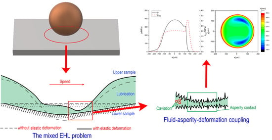
2.1. Analysis of Mixed EHL Problems

For rough contacts, when the clearance between two rough surfaces is limited, hydrodynamic lubrication and asperity contact exist at the same time. They produce elastic deformation. The elastic deformation influences the oil film thickness. The change in oil film thickness leads to a change in hydrodynamic support and asperity contact load.

The current solution is to analyze the single physical process involved in the problem first, and then consider the coupling between each physical field. The developed solution consists of a coupled hydrodynamic lubrication analysis, asperity contact analysis, and elastic deformation analysis. The way to couple these physical fields is to find the oil film thickness for which the asperity contact load, hydrodynamic support, and applied load are in equilibrium. The nomenclature for all symbols in the following sentences can be found in Nomenclature.

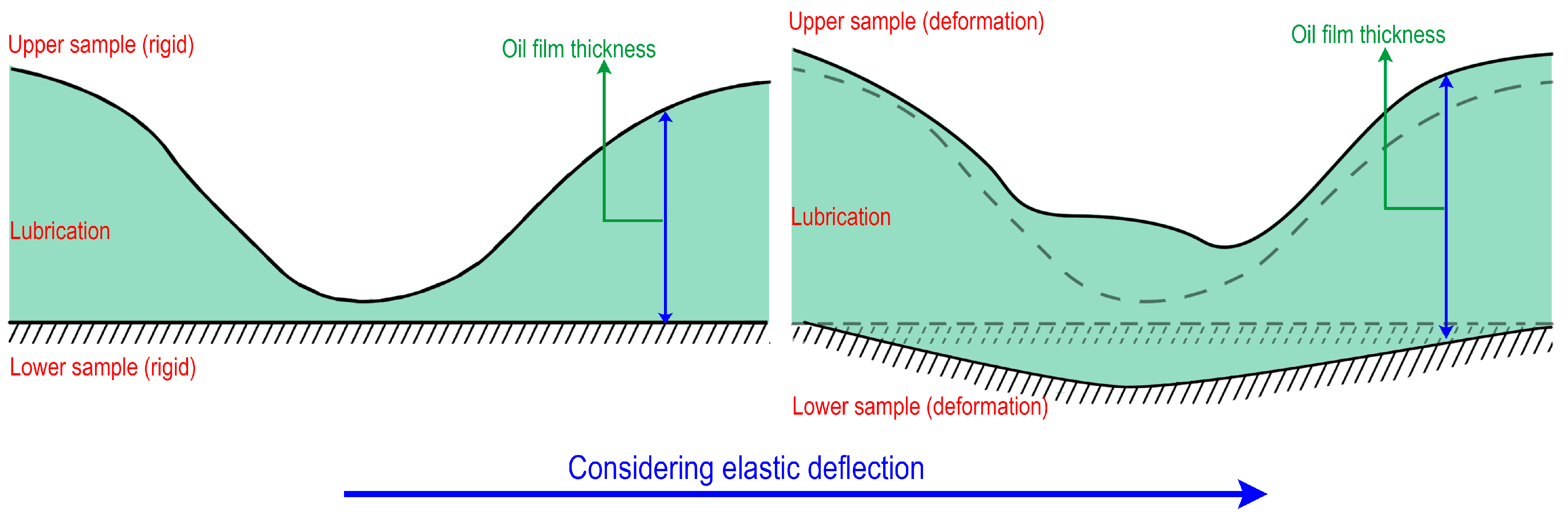
2.2. Elastic Deflection

The dependence of the oil film thickness on pressure (including hydrodynamic pressure and asperity contact pressure) cannot be neglected when the two mating bodies are elastic. As shown in Figure 1, the oil film thickness $h$ is given by the sum of $h_{prof}$ and $\delta$. The variable $h_{prof}$ is the oil film thickness in the case of rigid bodies. The deflection of the solid surfaces $\delta$ is expressed as $\delta ={\delta }_{hyd}+{\delta }_{asp}$. The variable ${\delta }_{hyd}$ is the deflection of the solid surface due to the hydrodynamic pressure, $\mathrm{while} {\delta }_{asp}$ is the deflection of the solid surface due to the asperity contact pressure:

$$h=h_{prof}+\delta =h_{prof}+{\delta }_{hyd}+{\delta }_{asp}$$

(1)

$${\delta }_{hyd}\left(x,y\right)=\frac{2}{\pi E^{\prime }}{{\displaystyle \iint }}_{\mathsf{\Omega }}\frac{p\left(s,t\right)}{\sqrt{{\left(x-s\right)}^2+{\left(y-t\right)}^2}}dsdt$$

(2)

$${\delta }_{asp}\left(x,y\right)=\frac{2}{\pi E^{\prime }}{{\displaystyle \iint }}_{\mathsf{\Omega }}\frac{p_{asp}\left(s,t\right)}{\sqrt{{\left(x-s\right)}^2+{\left(y-t\right)}^2}}dsdt$$

(3)

where the term ${\delta }_{hyd}$ and ${\delta }_{asp}$ can be calculated quickly based on a fast Fourier transform (FFT) method [12]. The variable $E^{\prime }$ is a combined elastic modulus of the contact bodies. It can be represented as:

$$\frac{1}{E^{\prime }}=\frac{1}{2}\left(\frac{1-{\upsilon }_1^2}{E_1}+\frac{1-{\upsilon }_2^2}{E_2}\right)$$

(4)

where $E_1$ and ${\upsilon }_1$ are the elastic modulus and Poisson’s ratio of the upper surfaces, respectively. $E_2$ and ${\upsilon }_2$ are for the lower surface.

Likewise, the equations above can be re-written as the summation of the products of influence coefficients $D_{i,j}^{k,l}$ and pressures $p\left(i,j\right)$ (or $p_{asp}\left(i,j\right)$). They are expressed as:

$${\delta }_{hyd}\left(x_k,y_l\right)=\frac{2}{\pi E^{\prime }}\sum _{i=1}^{N_{px}}\sum _{j=1}^{N_{py}}{D}_{i,j}^{k,l}p\left(i,j\right)\hspace{1em}\left(k=1,2\dots N_{dx},l=1,2\dots N_{dy}\right)$$

(5)

$${\delta }_{asp}\left(x_k,y_l\right)=\frac{2}{\pi E^{\prime }}\sum _{i=1}^{N_{px}}\sum _{j=1}^{N_{py}}{D}_{i,j}^{k,l}{p}_{asp}\left(i,j\right)\hspace{1em}\left(k=1,2\dots N_{dx},l=1,2\dots N_{dy}\right)$$

(6)

where $N_{px}$, $N_{py}$ are related to the pressures. They represent the total number of nodes in the $x$, $y$ directions. $N_{dx}$, $N_{dy}$ are related to the deformation. The influence coefficients $D_{i,j}^{k,l}$ can be calculated as:

$$\begin{gathered} D_{i,j}^{k,l}=\left(x_{k-i}+l_x\right)\ln \left[\frac{ℱ\left(y_{l-j}+l_y,x_{k-i}+l_x\right)}{ℱ\left(y_{l-j}-l_y,x_{k-i}+l_x\right)}\right] \\ \hspace{1em}\hspace{1em}\hspace{1em}\hspace{1em}\hspace{1em}\hspace{1em}\hspace{1em}\hspace{1em}\hspace{1em}\hspace{1em}\hspace{1em}+\left(y_{l-j}+l_y\right)\ln \left[\frac{ℱ\left(x_{k-i}+l_x,y_{l-j}+l_y\right)}{ℱ\left(x_{k-i}-l_x,y_{l-j}+l_y\right)}\right] \\ \hspace{1em}\hspace{1em}\hspace{1em}\hspace{1em}\hspace{1em}\hspace{1em}\hspace{1em}\hspace{1em}\hspace{1em}\hspace{1em}\hspace{1em}+\left(x_{k-i}-l_x\right)\ln \left[\frac{ℱ\left(y_{l-j}-l_y,x_{k-i}-l_x\right)}{ℱ\left(y_{l-j}+l_y,x_{k-i}-l_x\right)}\right] \\ \hspace{1em}\hspace{1em}\hspace{1em}\hspace{1em}\hspace{1em}\hspace{1em}\hspace{1em}\hspace{1em}\hspace{1em}\hspace{1em}\hspace{1em}+\left(y_{l-j}-l_y\right)\ln \left[\frac{ℱ\left(x_{k-i}-l_x,y_{l-j}-l_y\right)}{ℱ\left(x_{k-i}+l_x,y_{l-j}-l_y\right)}\right] \end{gathered}$$

(7)

as

$$ℱ\left(\mathrm{x},\mathrm{y}\right)=x+\sqrt[]{x^2+y^2}$$

(8)

where $l_x$ and $l_y$ are the half-lengths of the rectangular integration element. $x_{k-i}=x_k-x_i$ and $y_{l-j}=y_l-y_j$.

2.3. Fluid Mechanics

In order to predict the distribution of hydrodynamic lubrication, the two-scale model for fluid flow was employed here. A complementary formulation of the Reynolds equation needed to be adopted to solve the cavitation problem. The JFO (Jacobsson–Floberg–Olsson) [13,14] cavitation boundary condition was used in this model to consider the effect of cavitation from the perspective of a global scale. The classic flow factor methodology [15] was incorporated into this model to deal with the local (roughness) scale. The equation can be expressed as follows [16]:

$$\begin{array}{l}\frac{\partial }{\partial x}\left({\varphi }_x\frac{\rho }{\mu }{h}^3\frac{\partial p}{\partial x}\right)+\frac{\partial }{\partial y}\left({\varphi }_y\frac{\rho }{\mu }{h}^3\frac{\partial p}{\partial y}\right)\\ \hspace{1em}\hspace{1em}\hspace{1em}\hspace{1em}\hspace{1em}\hspace{1em}=12U_m{\varphi }_c\frac{\partial \left[\left(1-\theta \right)\rho h\right]}{\partial x}+12U_m\sigma \frac{\partial \left[\left(1-\theta \right)\rho {\varphi }_s\right]}{\partial x}\\ \hspace{1em}\hspace{1em}\hspace{1em}\hspace{1em}\hspace{1em}\hspace{1em}+12{\varphi }_c\frac{\partial \left[\left(1-\theta \right)\rho h\right]}{\partial t}\end{array}$$

(9)

With

$$p+\theta -\sqrt{p^2+{\theta }^2}=0$$

(10)

where $p$ is hydrodynamic pressure, and $\theta$ is the cavity fraction. The variable $h$ represents the oil film thickness, $\rho$ is the density of the lubricant, $\mu$ denotes the viscosity, $U_m=\frac{U_{upper}+U_{lower}}{2}$: $U_{upper}$ is the velocity of the upper surface, while $U_{lower}$ is the velocity of the lower surface. The variable $\sigma$ represents the equivalent surface roughness, which is obtained as $\sigma =\sqrt{{\sigma }_1^2+{\sigma }_2^2}$. The variables ${\varphi }_x$ and ${\varphi }_y$ are the pressure flow factors, and ${\varphi }_s$ represents the shear flow factor [15,17]. The variable ${\varphi }_c$ is the contact factor.

2.4. Lubricant Property

The lubricant viscosity is determined by various factors. Using the Roelands Equation [18], the effect of pressure on the viscosity can be characterized as:

$$\mu ={\mu }_{0}exp\left\{\left(ln{\mu }_0+9.67\right)\left[{\left(1+5.1\times {10}^{-9}p\right)}^{\alpha }-1\right]\right\}$$

(11)

where $\alpha$ is characteristics specific to particular lubricants, and is usually considered to be around 0.68.

In addition, the density-pressure relationship proposed by Dowson and Higginson [19] was adopted here. It reads:

$$\rho ={\rho }_0\left(1+\frac{0.6\times {10}^{-9}p}{1+1.7\times {10}^{-9}p}\right)$$

(12)

where ${\rho }_0$ is the lubricant density under atmospheric pressure.

2.5. Contact Mechanics

The asperity contact pressure can be obtained by the GT (Greenwood–Tripp) model [20]. The GT model is one of the multi-asperity models. The asperity contact pressure is given by:

$$p_{asp}=\frac{16\sqrt{2}\pi }{15}{\left(\eta \beta \sigma \right)}^2\sqrt{\frac{\sigma }{\beta }}\frac{E_1{E}_2}{E_2\left(1-{\upsilon }_1^2\right)+E_1\left(1-{\upsilon }_2^2\right)}{{\displaystyle \int }}_{\lambda }^{\infty }{\left(\overline{\xi }-\lambda \right)}^{2.5}{\varphi }^{*}\left(\overline{\xi }\right)d\overline{\xi }$$

(13)

where ${\varphi }^{*}\left(\overline{\xi }\right)$ is the normalized height distribution. The random variable $\xi$ is the combined roughness. $\overline{\xi }=\xi /\sigma$ and $\lambda =h/\sigma$. The variables $\eta \beta \sigma$ and $\sigma /\beta$ are the roughness-related parameters [21]. By generating $\varphi \left(\xi \right)$ with a known mean, $\sigma$, $S_k$, and $K_u$ can be found in the work of Kotwal et al. [22].

3. Method of Solution

In the simulation of the transient mixed EHL problem, due to the stiff nature of the problem, the results are more sensitive to the updated oil film thickness distribution. The oil film thickness distribution is influenced by the deformation induced by the asperity contact and hydrodynamic pressures. At the same time, the asperity contact and hydrodynamic pressures are also influenced by the distribution of oil film thickness. A robust and computational efficiency solution was urgently required.

In this paper, a novel solution was proposed to solve the mixed EHL problem. The EHL-FBNS algorithm was used to deal with the hydrodynamic lubrication, with cavitation and elastic deformation effects taken into consideration. The algorithm was first developed by Hansen et al. [23]. For the completeness of this article, the way of solving the EHL-FBNS algorithm using the Newton method is briefly recalled in the following sentences. For the lubrication model, there are two systems: $\mathit{F}\left(\mathit{p},\mathit{\theta }\right)=\mathit{p}+\mathit{\theta }-\sqrt{{\mathit{p}}^2+{\mathit{\theta }}^2}=\mathit{0}$ and $\mathit{G}\left(\mathit{p},\mathit{\theta }\right)=\mathit{A}\mathit{p}+\mathit{B}\mathit{\theta }+\mathit{c}=\mathit{0}$. After computing $\mathit{G}$ and $\mathit{F}$, the Newton–Raphson method can be used to determine the updates in pressure $\mathsf{\Delta }p$ and cavity fraction $\mathsf{\Delta }\theta$. Four Jacobian matrices are then constructed. They are ${\mathit{J}}_{\mathit{G},\mathit{p}}=\mathit{A}$, ${\mathit{J}}_{\mathit{G},\mathit{\theta }}=\mathit{B}$, ${\mathit{J}}_{\mathit{F},\mathit{p}}=\frac{\mathit{\partial }\mathit{F}}{\mathit{\partial }\mathit{p}}$, and ${\mathit{J}}_{\mathit{F},\mathit{\theta }}=\frac{\mathit{\partial }F}{\mathit{\partial }\theta }$.

$$\mathit{J}\left[\begin{array}{c}\Delta {\mathit{p}}^k\\ \Delta {\mathit{\theta }}^k\end{array}\right]=\left[\begin{array}{cc}{\mathit{J}}_{\mathit{F},\mathit{p}}& {\mathit{J}}_{\mathit{F},\mathit{\theta }}\\ {\mathit{J}}_{\mathit{G},\mathit{p}}& {\mathit{J}}_{\mathit{G},\mathit{\theta }}\end{array}\right]\left[\begin{array}{c}\Delta {\mathit{p}}^k\\ \Delta {\mathit{\theta }}^k\end{array}\right]=-\left[\begin{array}{c}\mathit{F}\\ \mathit{G}\end{array}\right]$$

(14)

The Jacobian matrices ${\mathit{J}}_{\mathit{F},\mathit{p}}$ and ${\mathit{J}}_{\mathit{F},\mathit{\theta }}$ are the diagonal matrices. The values of the elements on the diagonal are $J_{F,p}=1-\frac{p}{\sqrt{p^2+{\theta }^2}}$, and $J_{F,\theta }=1-\frac{\theta }{\sqrt{p^2+{\theta }^2}}$. For the EHL-FBNS algorithm, when elastic deformation is taken into account, the pressure Jacobian ${\mathit{J}}_{\mathit{G},\mathit{p}}$ of the Reynolds equation should be treated specially. The operation is to consider the dependence $\mathit{h}$ by inserting it into $\mathit{c}$, thus creating the matrix A. Due to the kernel function, this operation results in A being a full matrix. It causes unstable behavior in the iteration process. In this case, the influence of elastic deformation on matrix A is approximately represented by its main diagonal.

The influence coefficient $D\left(i,j\right)$ only depends on the grid geometry. When $D\left(0,0\right)$ is aligned with $p\left(i,j\right)$, ${\delta }_{hyd}\left(i,j\right)$ can be approximately equal to the following expression:

$$\begin{array}{c}{\delta }_{hyd}\left(i,j\right)\approx D\left(0,0\right)p\left(i,j\right)+D\left(-1,0\right)p\left(i+1,j\right)+D\left(1,0\right)p\left(i-1,j\right)\\ \hspace{1em}\hspace{1em}\hspace{1em}+D\left(0,1\right)p\left(i,j-1\right)+D\left(0,-1\right)p\left(i,j+1\right)\end{array}$$

(15)

as

$$h=\underset{fixed}{\underbrace{h_{prof}+{\delta }_{asp}}}+\underset{changed}{\underbrace{{\delta }_{hyd}}}$$

(16)

The following two terms from Equation (9) can be discretized:

$$\begin{gathered} \begin{array}{l}\frac{\partial \left[\rho h\right]}{\partial x}=\frac{{\rho }_P{h}_P-{\rho }_W{h}_W}{dx}=\frac{{\rho }_P{\delta }_{hyd,P}-{\rho }_W{\delta }_{hyd,W}}{dx}\\ \approx \frac{\hspace{1em}{\rho }_P\left[\begin{array}{c}D\left(0,0\right)p\left(i,j\right)+D\left(-1,0\right)p\left(i+1,j\right)+D\left(1,0\right)p\left(i-1,j\right)\\ +D\left(0,1\right)p\left(i,j-1\right)+D\left(0,-1\right)p\left(i,j+1\right)\end{array}\right] \\ -{\rho }_W\left[\begin{array}{c}D\left(-1,0\right)p\left(i,j\right)+D\left(-2,0\right)p\left(i+1,j\right)+D\left(0,0\right)p\left(i-1,j\right)\\ +D\left(-1,1\right)p\left(i,j-1\right)+D\left(-1,-1\right)p\left(i,j+1\right)\end{array}\right]}{dx}\end{array} \end{gathered}$$

(17)

In addition, ${\delta }_{hyd}\left(i,j\right)$ can be used to obtain the Jacobians of the term $\frac{\partial \left[\rho h\right]}{\partial t}$ in a similar fashion. In this way, the matrix ${\mathit{J}}_{\mathit{G},\mathit{p}}$ with the effect of deformation in consideration can be obtained. Later, in order to make it well-conditioned, the Jacobian $\mathit{J}$ should be restructured into a new Jacobian ${\mathit{J}}^{\prime }$ by swapping the corresponding columns when finding $J_{F,p}<J_{F,\theta }$.

$${\mathit{J}}^{\prime }\left[\begin{array}{c}\Delta \mathit{a}\\ \Delta \mathit{b}\end{array}\right]=\left[\begin{array}{c}{\mathit{A}}_{\mathit{F}}{\mathit{B}}_{\mathit{F}}\\ {\mathit{A}}_{\mathit{G}}{\mathit{B}}_{\mathit{G}}\end{array}\right]\left[\begin{array}{c}\Delta \mathit{a}\\ \Delta \mathit{b}\end{array}\right]=-\left[\begin{array}{c}\mathit{F}\\ \mathit{G}\end{array}\right]$$

(18)

$$\{\begin{array}{c}\left({\mathit{B}}_{\mathit{G}}-{\mathit{A}}_{\mathit{G}}{\mathit{A}}_{\mathit{F}}^{-\mathbf{1}}{\mathit{B}}_{\mathit{F}}\right)\mathsf{\Delta }\mathit{b}=-\mathit{G}+{\mathit{A}}_{\mathit{G}}{\mathit{A}}_{\mathit{F}}^{-\mathbf{1}}\mathit{F}\\ \mathsf{\Delta }\mathit{a}={\mathit{A}}_{\mathit{F}}^{-\mathbf{1}}\left(-\mathit{F}-{\mathit{B}}_{\mathit{F}}\mathsf{\Delta }\mathit{b}\right)\end{array}$$

(19)

After obtaining the solutions $\mathsf{\Delta }\mathit{a}$ and $\mathsf{\Delta }\mathit{b}$, the updated increment vectors $\mathsf{\Delta }\mathit{p}$ and $\mathsf{\Delta }\mathit{\theta }$ can be obtained by reverse reordering the variables $\Delta \mathit{a}$ and $\Delta \mathit{b}$. According to equations $\mathit{p}=\mathit{p}+\Delta \mathit{p}$ and $\mathit{\theta }=\mathit{\theta }+\Delta \mathit{\theta }$, the new $\mathit{p}$ and $\mathit{\theta }$ are obtained and can be used to calculate the Jacobian matrices again. The solution continues until the following evaluation criterion $A$ is satisfied.

$$Max\left(\left|\Delta \mathit{p}\right|, \left|\Delta \mathit{\theta }\right|, \left|\mathit{F}\right|, \left|\mathit{G}\right|\right)<{10}^{-6}$$

(20)

It should be noted that solving the EHL-FBNS algorithm is computationally efficient. It was reported that the execution time of the presented algorithm scales almost reached $Nlog\left(N\right),$ where $N$ is the number of computational grid points. To make it robust, the relaxation factors can be used in the update of $p$ and $\theta$ by $\mathit{p}=\mathit{p}+{\omega }_1\Delta \mathit{p}$ and $\mathit{\theta }=\mathit{\theta }+{\omega }_1\Delta \mathit{\theta }$. The variable ${\omega }_1$ can be set between 0.05 and 1 to balance the convergence speed and stability. For more detailed information, the reader can refer to the work of Hansen et al. [23].

The coupling of fluid and deformation can be studied by solving the EHL-FBNS algorithm, while the coupling of asperity contact and deformation can be analyzed by the following method. Equation (13) cannot be directly employed in order to correct the MOFT as a function of the contact pressure $p_{asp}$, since a severe non-linear problem usually arises. For the asperity contact deformation coupling problem, the non-linear system of equations can be described as:

$$\mathit{Q}=\mathit{f}\left(\mathit{h}\right)=\mathit{h}-\underset{fixed}{\underbrace{\left({\mathit{h}}_{\mathit{p}\mathit{r}\mathit{o}\mathit{f}}+{\mathit{\delta }}_{\mathit{h}\mathit{y}\mathit{d}}\right)}}-\underset{changed}{\underbrace{{\mathit{\delta }}_{\mathit{a}\mathit{s}\mathit{p}}\left(\mathit{h}\right)}=\mathbf{0}}$$

(21)

$${\mathit{J}}^{\prime }\mathsf{\Delta }\mathit{h}={{\mathit{J}}^{\prime }}_{\mathit{Q},\mathit{h}}\mathsf{\Delta }\mathit{h}=\left[\frac{\mathit{\partial }\mathit{h}}{\mathit{\partial }\mathit{h}}-\frac{\mathit{\partial }{\mathit{\delta }}_{\mathit{a}\mathit{s}\mathit{p}}\left(\mathit{h}\right)}{\mathit{\partial }\mathit{h}}\right]\mathsf{\Delta }\mathit{h}=-\mathit{Q}$$

(22)

$$\mathit{h}=\mathit{h}+{\omega }_2\mathsf{\Delta }\mathit{h}$$

(23)

The variable ${\omega }_2$ is the relaxation factor. The variable ${\delta }_{asp}$ is influenced by the $p_{asp}$. However, $p_{asp}$ is influenced by $h$. The relationship can be expressed as: $\frac{1}{h}\propto p_{asp}\propto {\delta }_{asp}$. In order to prevent ${{\mathit{J}}^{\prime }}_{Q,h}$ from becoming a full matrix, $D\left(0,0\right)$ must be aligned with $p_{asp}\left(i,j\right)$, and ${\delta }_{asp}$ can be approximately equal to the following expression:

$$\begin{array}{c}{\delta }_{asp}\left(i,j\right)\approx D\left(0,0\right)p_{asp}\left(i,j\right)+D\left(-1,0\right)p_{asp}\left(i+1,j\right)+D\left(1,0\right)p_{asp}\left(i-1,j\right)\\ \hspace{1em}\hspace{1em}\hspace{1em}+D\left(0,1\right)p_{asp}\left(i,j-1\right)+D\left(0,-1\right)p_{asp}\left(i,j+1\right)\end{array}$$

(24)

Then:

$$\begin{array}{c}\frac{\partial {\delta }_{asp}\left(i,j\right)}{\partial h}\approx D\left(0,0\right)\frac{\partial p_{asp}\left(i,j\right)}{\partial h}+D\left(-1,0\right)\frac{\partial p_{asp}\left(i+1,j\right)}{\partial h}\\ \hspace{1em}\hspace{1em}\hspace{1em}\hspace{1em}\hspace{1em}\hspace{1em}\hspace{1em}\hspace{1em}+D\left(1,0\right)\frac{\partial p_{asp}\left(i-1,j\right)}{\partial h}+D\left(0,1\right)\frac{\partial p_{asp}\left(i,j-1\right)}{\partial h}\\ \hspace{1em}+D\left(0,-1\right)\frac{\partial p_{asp}\left(i,j+1\right)}{\partial h}\end{array}$$

(25)

where $\frac{\partial p_{asp}\left(i,j\right)}{\partial h}$ represents the contact stiffness. In order to tackle this non-linearity, the Newton–Raphson method can also be employed. The iteration continues until the following evaluation criterion $B$ is satisfied:

$$Max\left(\left|\mathit{Q}\right|, \left|\mathsf{\Delta }\mathit{h}\right|\right)<{10}^{-6}$$

(26)

In this way, the coupling of fluid and deformation and the coupling of asperity contact and deformation can be solved separately to tackle the non-linearity of the mixed EHL problem. Later, the effect of fluid, asperity contact, and deformation should be coupled. The whole loop needs to be continued until evaluation criterion $C$ is satisfied.

$$p_{tota}=p+p_{asp}$$

(27)

$$Max\left(\left|p_{tota}-p_{tota}^{pre}\right|, \left|h-h^{pre}\right|\right)<{10}^{-6}$$

(28)

The subscript $pre$ denotes that the elements are under the previous cycle. In general, only a limited number of iterations are required before the evaluation criterion is satisfied.

For a mixed EHL problem, a constant applied load is prescribed. Therefore, another loop should be added to find the oil film thickness when the asperity contact load, hydrodynamic support, and applied load are in equilibrium. The balance equation can be described as

$$f\left(h_0\right)=W_{asp}+W_{hyd}-W_{load}=0$$

(29)

A Newton method can be used to find the value of $h_0$, based on the following equation: $h_0=h_0-\frac{f\left(h_0\right)}{f^{\prime }\left(h_0\right)}$. It is different from obtaining the derivative of $f\left(h_0\right)$. The Secant method can be used:

$$h_0=h_0-\frac{f\left(h_0\right)dh}{\left(f\left(h_0+dh\right)-f\left(h_0\right)\right)}$$

(30)

In this way, the load balance can be obtained quickly. The sequence of computation is summarized in Figure 2.

4. Results and Discussion

In order to assess the performance of the proposed method, it should be employed in some cases from other literature to verify its effectiveness. The first case is the parallel slider with a varying number of trapezoidal pockets. The comparison results are given in Section 4.1. Subsequently, a transient case should be carried out to evaluate the performance of the proposed method in unsteady mixed EHL conditions. One experimental numerical literature case was chosen due to the availability of the data. The performance of the ball-on-disc conjunction with moving texture was analyzed. The comparison results and discussion are given in Section 4.2.

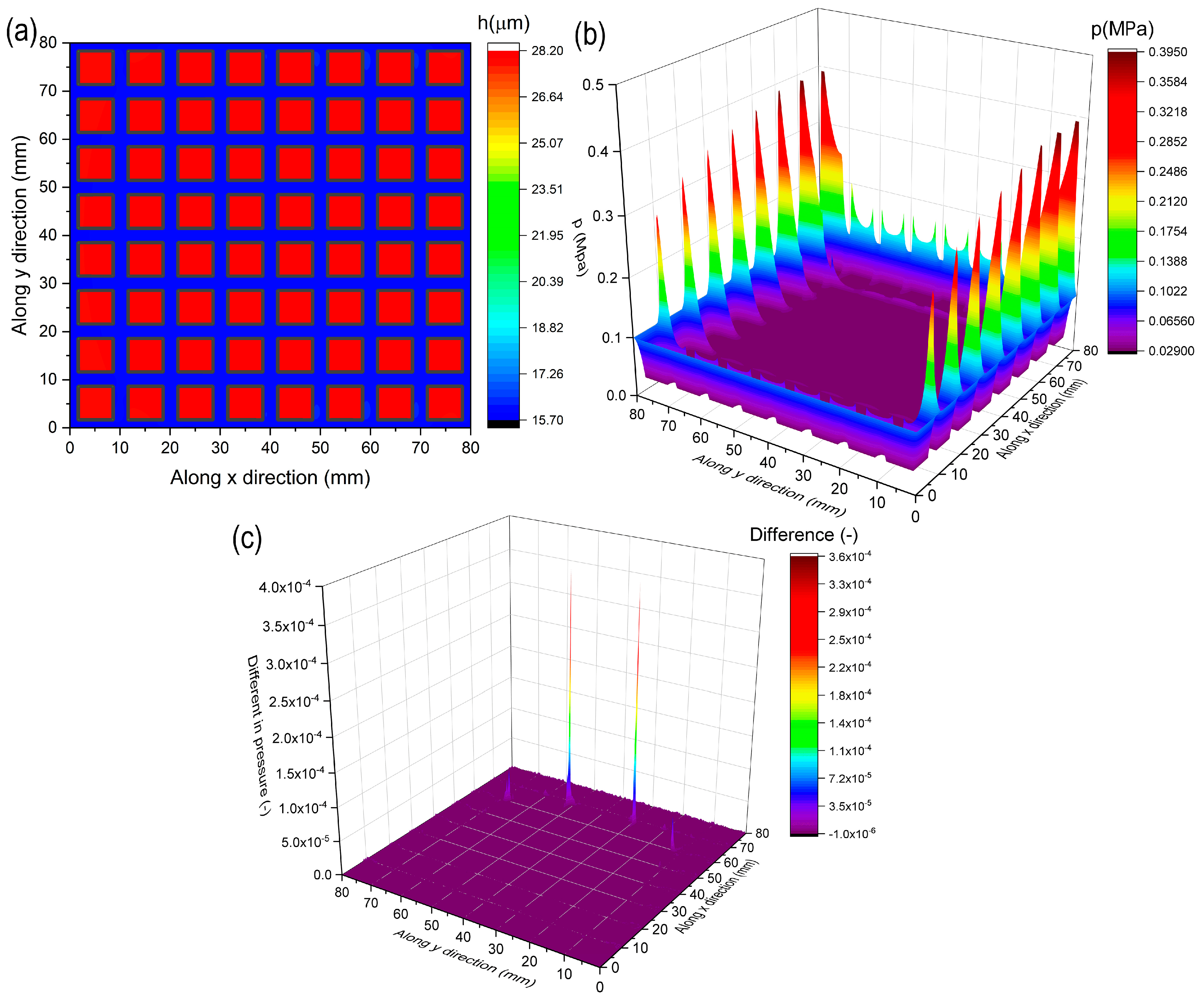
4.1. Slider with a Varying Number of Trapezoidal Pockets

The simulation conditions can be found in the works of Woloszynski et al. [24] and Hansen et al. [23]. The simulation results are given in Figure 3. To quantify the difference in the results of hydrodynamic pressure from the current method and the reference, the term is defined as: $\frac{p_{cur}-p_{ref}}{p_{ref}}\times 100\%$. The result obtained by the present method ($p_{cur}$) matched well with the result available in the literature ($p_{ref}$). It was found that only a difference of 0.0004% in pressure distribution between the current method (setting ${\varphi }_x,{\varphi }_y=1$, ${\varphi }_c=1$ and ${\varphi }_s=0$) and the one presented in Ref. [23] was detected.

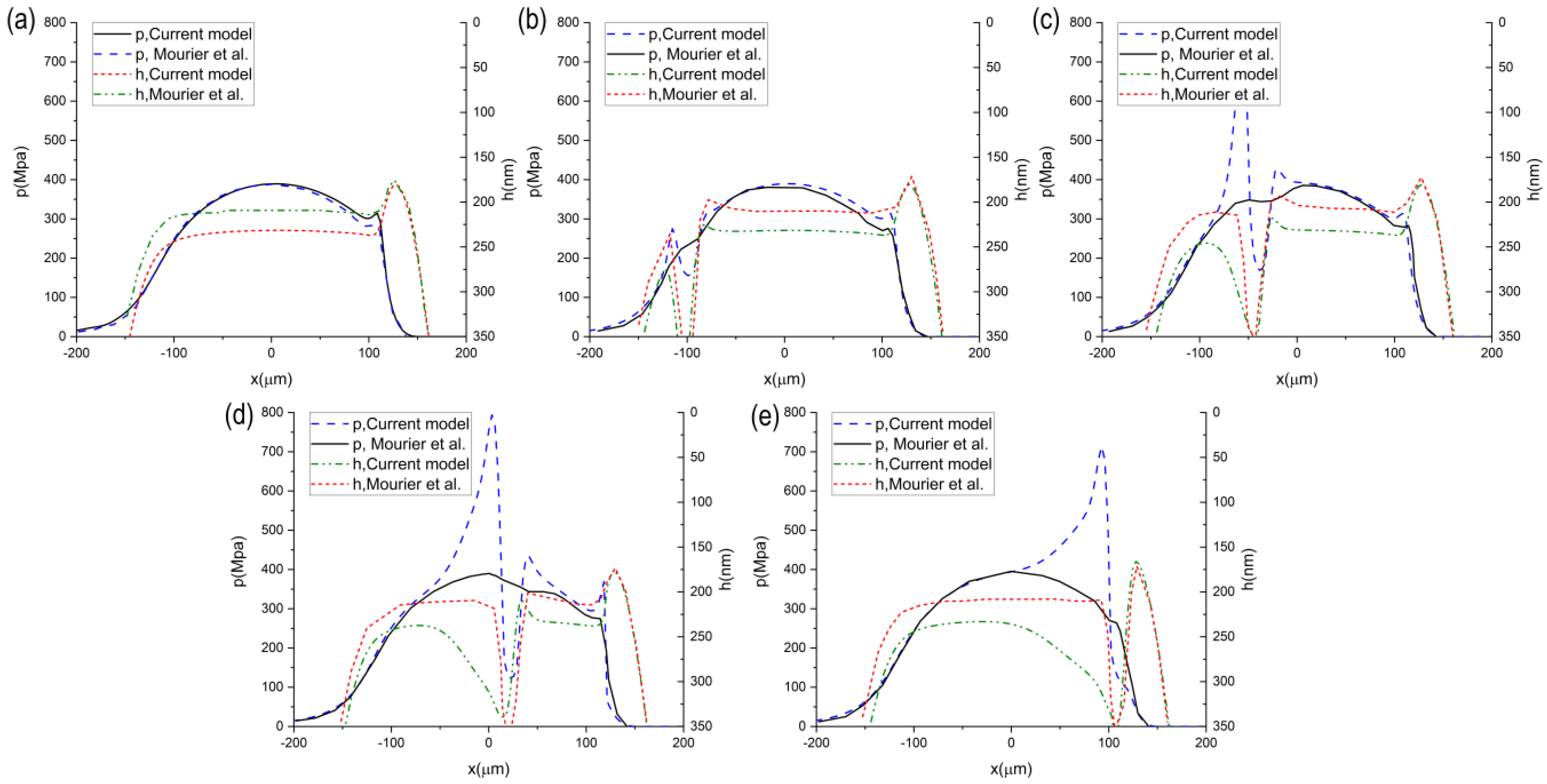
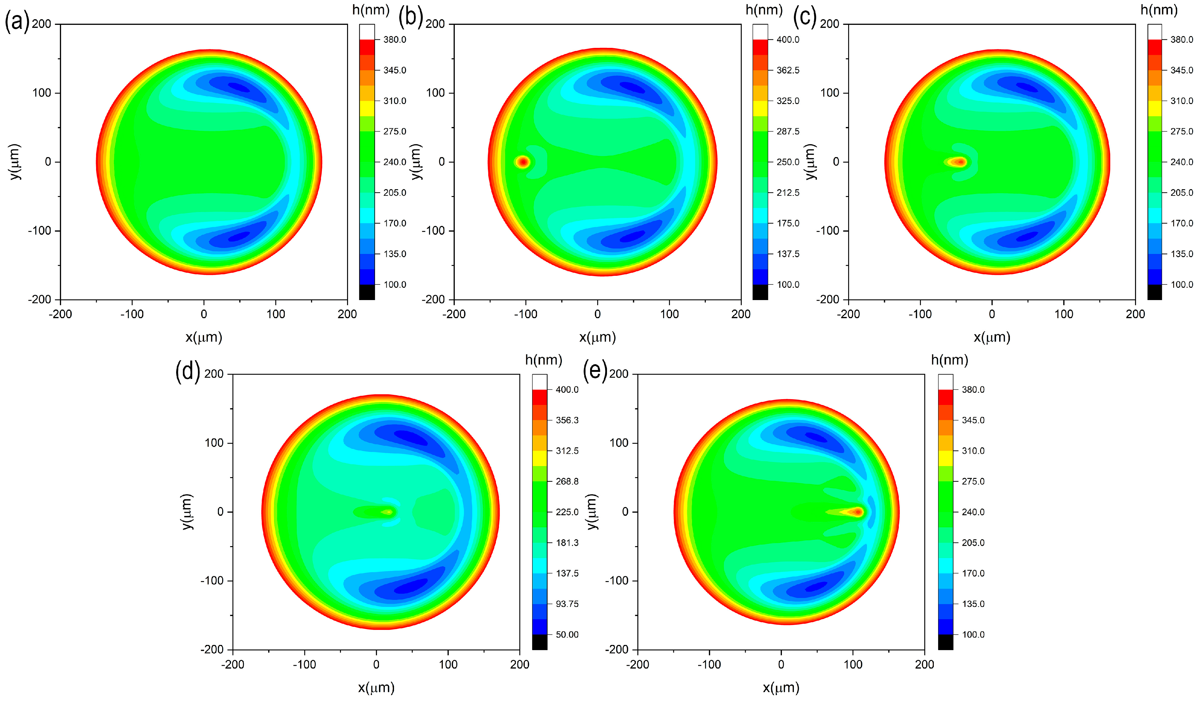
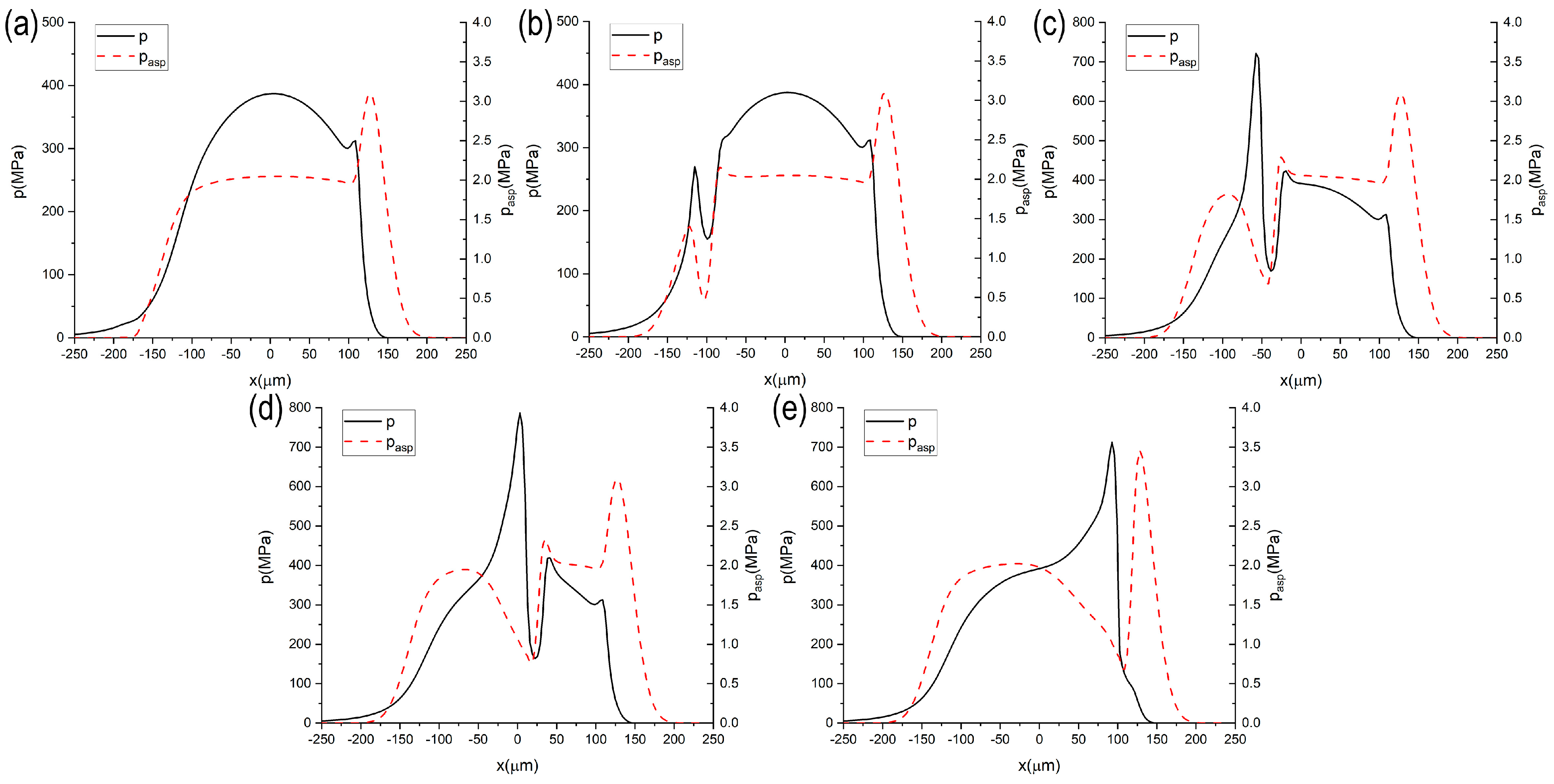
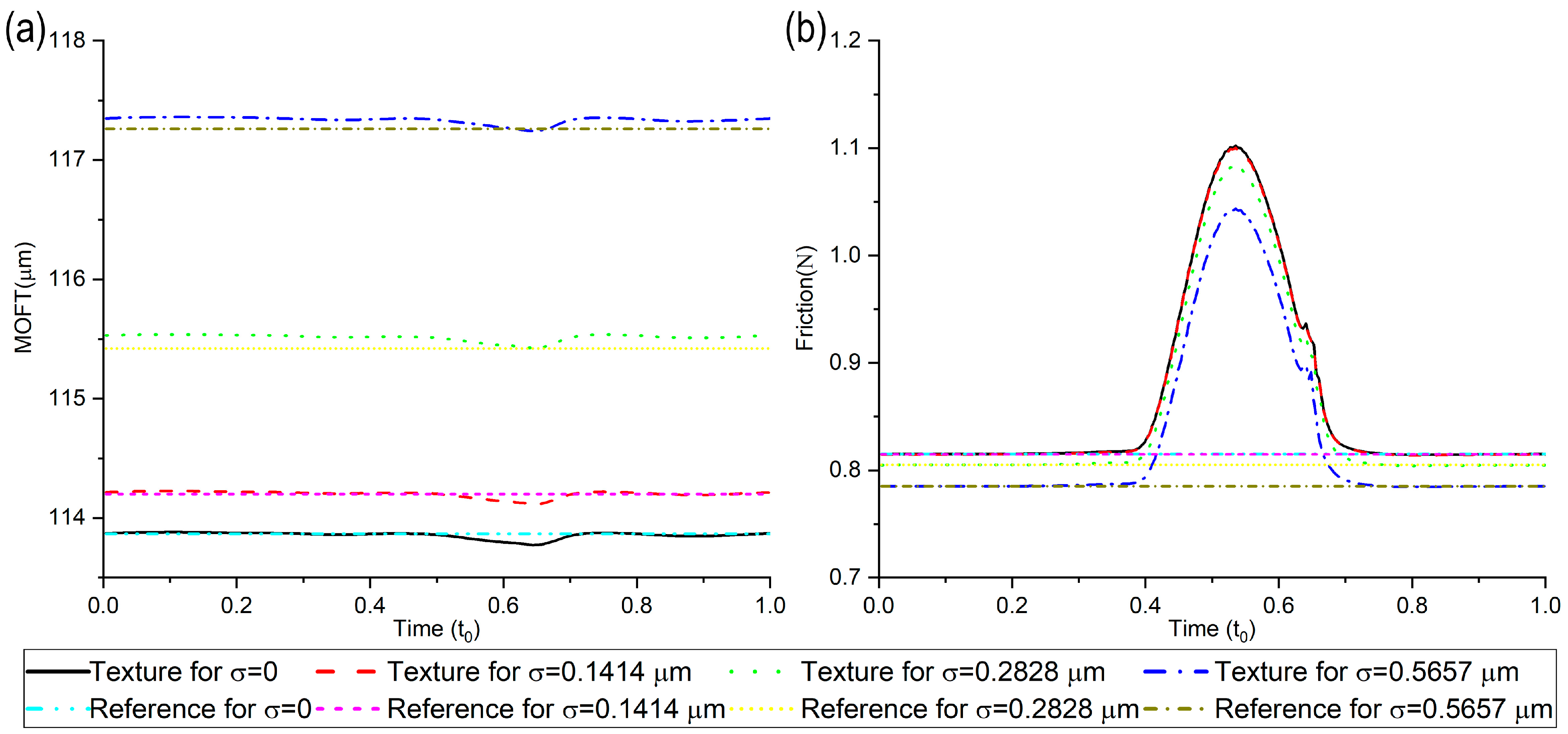
4.2. Point Contact with or without Moving Texture

The classical EHL case of point contact under pure rolling conditions was tested in the following sentences. The simulation conditions for point contact with and without texture are listed in

Table 1. Simulation conditions for point contact.

Parameter	Value	Unit
$p_{cav}$	0	Pa
$W_{load}$	15	N
$E^{\prime }$	110	GPa
${\mu }_0$	0.25	Pa.s
${\rho }_0$	850	$\mathrm{Kg}/{\mathrm{m}}^3$
a	136.5	$\mathsf{\mu }\mathrm{m}$
$L_x$	6a	-
$L_y$	6a	-
$U_{upper}$	0.09	$\mathrm{m}/\mathrm{s}$
$U_{lower}$	0.09	$\mathrm{m}/\mathrm{s}$
r	15.5	$\mathsf{\mu }\mathrm{m}$
d	175	$\mathrm{nm}$

. The term $r$ is the radius of texture. The term $d$ is its depth. The term $a$ is the half-width of Hertzian contact. The term $p_{cav}$ is the cavitation pressure.

In order to understand the efficiency of the proposed method, two cases of steady-state simulations were conducted. For the sake of simplicity, the ball/disc contact with no texture was considered. The rigid body displacement was prescribed to avoid adjusting the rigid body displacement in order to achieve the load balance. The expression of oil film thickness for the point contact is given as follows:

$$h\left(x,y,t\right)=\underset{h_{prof}}{\underbrace{h_0+\frac{x^2}{2R_x}+\frac{y^2}{2R_y}}}+\delta$$

(31)

where $h_0$ is the rigid body displacement. It is noteworthy that $h_0$ is not the MOFT, since the deformation induced by pressure was considered.

Case 1 is for smooth contact, while Case 2 is for rough contact. For smooth contact, the roughness values of the upper and lower samples are set to 0. It means that the asperity contact is neglected. For the rough contact, the roughness values of the upper and the lower sample are all 0.2 $\mathsf{\mu }\mathrm{m}$. The asperity contact algorithm should be introduced in order to mimic a mixed-lubrication regime correctly. In particular, at each iterative step, the distributions of the hydrodynamic pressure and the oil film thickness are evaluated; the oil film thickness between the mating surfaces is then computed and used to detect if asperity contact occurs. The resulting pressure vector, $p_{asp}$, presents non-null values where asperity contact occurs. In general, when the oil film thickness is thinner, the calculation is more difficult to converge. For Case 1 and Case 2, $h_0$ is set to 0.

Moreover, two different methods were employed, including the standard and presented methods. The FBNS method was used in the standard method to obtain pressure convergence. The relaxation method was used to achieve the convergence of the total pressure after the asperity contact pressure was calculated. The expression is given as: $p_{tota}={\omega }_0{p}_{tota}+\left(1-{\omega }_0\right)p_{tota}^{pre}$. The variable ${\omega }_0$ has a limited value. It ranges from 0.01 to 0.2. In the presented method, the EHL-FBNS method was used to obtain pressure convergence by considering the deformation and cavitation. The Newton iteration method was used to obtain asperity contact pressure by considering deformation. The effect of fluid, asperity contact, and deformation was coupled by setting the deformation induced by asperity contact pressure as a constant when the hydrodynamic pressure was calculated, and by setting the deformation caused by hydrodynamic pressure as a constant when calculating asperity contact pressure.

These tests were run using a computer with an Intel Core i7-11700 CPU with each core clocked at 2.50 GHz and 48 Gb of memory. Since $\left({\mathit{B}}_{\mathit{G}}-{\mathit{A}}_{\mathit{G}}{\mathit{A}}_{\mathit{F}}^{-\mathbf{1}}{\mathit{B}}_{\mathit{F}}\right)\mathsf{\Delta }\mathit{b}=-\mathit{G}+{\mathit{A}}_{\mathit{G}}{\mathit{A}}_{\mathit{F}}^{-\mathbf{1}}\mathit{F}$ in Equation (19) would be solved in both methods, each solution of this equation was regarded as one iteration.

Table 2. The number of iterations and computation time (CPU time (seconds)) required by different methods to calculate the mixed EHL problem for different cases.

Parameter	Case	Standard Method			Current Method
		${\mathit{\omega }}_0=0.2$	${\mathit{\omega }}_0=0.1$	${\mathit{\omega }}_0=0.01$	${\mathit{\omega }}_1=0.2$	${\mathit{\omega }}_1=0.1$	${\mathit{\omega }}_1=0.05$
Number of iterations	1	1582	2137	10667	56	103	210
	2	1528	2043	9982	231	460	941
CPU time (s)	1	66.55	92.06	500.02	2.86	4.91	9.58
	2	62.47	87.02	472.69	11.16	19.91	39.17

shows the number of iterations and computation time (CPU time (s)) required by different methods to calculate the mixed EHL problem for the two cases. It can be found that for the current method, the total iteration was far less than that required for the standard method. It resulted in the reduction in CPU time for the current method. Meanwhile, it was found that both the number of iterations and CPU times were influenced by the relaxation factor. A large relaxation factor can converge quickly, and a low relaxation factor can ensure the stability of the calculation. It appears that only 2–17% of the calculation time was required when the current method was employed.

Later, the simulation of the ball/disc conjunction with the texture on the disc was carried out. The ball/disc conjunction with the texture on the disc constitutes a scientific challenge from the numerical perspective. The simulation of the ball/disc conjunction with texture on the disc is a multiscale problem. There are three different scales. They are the global scale, texture scale, and roughness scale. There is a large difference in scale between the global contact dimensions and local surface properties. Local surface properties (including textures or roughness) play an essential role in the efficiency of lubricated contacts. In addition, the dynamical behavior of the ball/disc conjunction is completely different depending on whether the texture is on the ball or the disc. If the texture is on the disc, the texture cells enter the contact from one side, move under the disc, and leave the contact on the opposite side. For the ball/disc conjunction with the texture on the disc, the gap can be expressed as:

$$h\left(x,y,t\right)=\{\begin{array}{cc}{h}_0+\frac{x^2}{2R_x}+\frac{y^2}{2R_y}+\delta & \\ +dcos\left(\frac{\pi }{2}\frac{\sqrt{{\left(x-u_{tex}t\right)}^2+y^2}}{1.2r}\right)e^{-2\left(\frac{\sqrt{{\left(x-u_{tex}t\right)}^2+y^2}}{1.2r}{)}^2\right)}& if-3a\le x\le 3a\hfill \\ h_0+\frac{x^2}{2R_x}+\frac{y^2}{2R_y}+\delta & otherwise\hfill \end{array}$$

(32)

The gap (or oil film thickness) changes with time.

Next, the present model’s results were compared to Mourier et al.’s results [25]. It is noteworthy the roughness values of the ball and the disc were set to 0 here, since the asperity contact load was not considered in the simulated results of Mourier et al. [25]. Meanwhile, by setting ${\varphi }_x,{\varphi }_y=1$, ${\varphi }_c=1$, and ${\varphi }_s=0$, the effect of roughness on lubrication was not considered, in order to keep consistent with the reference. Figure 4 shows the results of the present model compared with the results from Mourier et al. [25]. At the first texture position, it was found that the results from the current method agreed well with the simulated results of Mourier et al. At the first texture position (shown in Figure 4a), the texture was just entering the ball/disc conjunction. Most of the domain was still unaffected by the texture. When the texture introduced unsteady effects at positions (b)–(e), the distributions of oil film thickness stayed closer to the results of Mourier et al. The differences in the results of the current model and Mourier et al. were limited.

Figure 5 shows the hydrodynamic pressure distribution for the ball-on-disc conjunction with moving texture. The distribution of the oil film thickness for the ball-on-disc conjunction with moving texturing can be found in Figure 6. According to the results, due to the limited texture dimension, it appeared that the influence of moving texturing was limited. The influence could only be found in the texture and the area around the texture. As shown in Figure 4b–e, in the area in front and at the side of the texture, there was a local constriction in the oil film thickness. Trailing effects in the area behind the texture led to a locally enlarged oil film thickness. It resulted in improved lubricating conditions. It was because that lubricant was drawn out of the texture by elastic deformation. It contributed to additional hydrodynamic pressure, as shown in Figure 5. As shown in Figure 6, the MOFT was around 0.1 $\mathsf{\mu }\mathrm{m}$. The oil film thickness around the texture was changed, due to the existence of texture and deformation. It led to a change in pressure distribution. It was found that the pressure peak was significantly improved when the texture was moving within the Hertz contact range.

Later, in order to evaluate the effect of roughness on the performance of ball/disc contact and find the influence of fluid–solid coupling, the roughness values of the ball/disc were set as 0.1 $\mathsf{\mu }\mathrm{m}$, 0.2 $\mathsf{\mu }\mathrm{m},$ and 0.4 $\mathsf{\mu }\mathrm{m}$. The detailed parameters are given in

Table 3. The simulation conditions for the fluid–solid coupling.

Parameters	Value	Unit
Roughness of ball	0.1, 0.2, 0.4	$\mathsf{\mu }\mathrm{m}$
Roughness of disc	0.1, 0.2, 0.4	$\mathsf{\mu }\mathrm{m}$
$\eta \beta \sigma$	0.04	--
$\sigma /\beta$	0.001	--

. In other words, the comprehensive roughnesses were 0.1414 $\mathsf{\mu }\mathrm{m}$, 0.2828 $\mathsf{\mu }\mathrm{m}$, and 0.5657 $\mathsf{\mu }\mathrm{m}$, respectively. Figure 7 shows the distributions of the hydrodynamic pressure and asperity contact pressure along the center liner of the ball/disc conjunction with moving texture when the comprehensive roughness was 0.2828 $\mathsf{\mu }\mathrm{m}$. It can be found that asperity contact pressure was limited. It was because the roughness was limited. The asperity contact pressure arises when the oil film thickness is less than three times the comprehensive surface roughness. Figure 8 shows the distributions of the hydrodynamic pressure, asperity contact pressure, and oil film thickness for the ball/disc conjunction with moving texture. As shown in Figure 8, asperity contact occurred in the Hertz contact zone for the point contact problem. Textures changed lubricating conditions at the local level. Each pocket “carried” its pressure field with it as it moved to the right. Due to lubricant being squeezed out of the textures by elastic deformation, the trailing effects led to a local oil film thickness enlargement. This may have reduced the asperity contact load. The asperity contact-induced friction could be reduced. Furthermore, it was found that additional constrictions occurred in the front and on the sides of the textures. The same phenomenon was also found in the work of Marian et al. [26]. These may lead to higher material fatigue and wear.

Moreover, Figure 9 shows the variation of MOFT and friction with time for different roughness values along the passage of one individual texture under the ball. It is worthy to note that friction was evaluated based on the following expression:

$$f_{tot}={\displaystyle \iint }\tau +{\kappa }_{asp}{p}_{asp}dxdy$$

(33)

$$\tau =-\left(1-\theta \right)\mu \frac{U}{h}\left({\varphi }_f+{\varphi }_{fs}\right)+\left(1-\theta \right){\varphi }_{fp}\frac{h}{2}\frac{\partial p}{\partial x}$$

(34)

The total friction $f_{tot}$ consists of the viscous friction $f_{vis}$ and the asperity contact friction $f_{asp}$. The parameters ${\varphi }_f$, ${\varphi }_{fs}$ and ${\varphi }_{fp}$ are the friction-induced flow factors, and ${\kappa }_{asp}$ is the boundary friction coefficient. A value of ${\kappa }_{asp}=0.1$ was adopted in this work. The results of the untextured ball/disc conjunction were regarded as references. As shown in Figure 9, the textured disc performed better than the untextured one. The MOFT and friction results strongly depended on the relative position of the texture with respect to the ball. When the roughness was increased, a local oil film thickness enlargement, as well as reduced solid–solid contact, was found. It appears that friction was decreased with the increased roughness. It indicates that the smaller roughness does not guarantee better tribological performance.

5. Conclusions

This present study developed a novel solution for mixed EHL analysis for engineering applications to tackle the non-linearity of the mixed EHL problem. The current solution is to analyze the single physical process involved in the problem first and then consider the coupling between each physical field. Two parts of the elastic deformation were considered. The hydrodynamic pressure-induced deformation was obtained by the unsteady EHL-FBNS solver by considering both mass-conserving cavitation and elastic deformation. The Newton–Raphson method was employed to obtain the asperity contact pressure-induced deformation. The proposed methodology was validated against relevant results in other literary works. The following conclusions were drawn:

The current method is one robust and efficient method. According to the result, for the current method, the total iteration is far less than that required for the standard method. The relaxation factor is an essential factor that can influence the calculation efficiency. A large relaxation factor can converge quickly, and a low relaxation factor can ensure the stability of the calculation. It appears that only 2–17% of the calculation time is required when the current method is employed.

Transient EHL simulations agree well with reference results. For the ball/disc conjunction with moving texturing, the relative position of the micro-texture has a strong influence on the resulting lubrication conditions and consequent friction and wear. The developed simulation can effectively track the tribological behavior of friction pairs with reduced dependence on experimental work. The employment of the presented method is recommended for the modeling of engineering applications under heavy loading.

References

1. Chen, S.; Yin, N.; Cai, X.; Zhang, Z. Iteration framework for solving mixed lubrication computation problems. Front. Mech. Eng. 2021, 16, 635–648. [Google Scholar] [CrossRef]
2. Zhu, D.; Hu, Y.-Z. The study of transition from elastohydrodynamic to mixed and boundary lubrication. In The Advancing Frontier of Engineering Tribology, Proceedings of the 1999 STLE/ASME HS Cheng Tribology Surveillance; American Society of Mechanical Engineers: New York, NY, USA, 1999; pp. 150–156. [Google Scholar]
3. Hu, Y.-Z.; Zhu, D. A Full Numerical Solution to the Mixed Lubrication in Point Contacts. J. Tribol. 2000, 122, 1–9. [Google Scholar] [CrossRef]
4. Wang, W.Z.; Wang, H.; Liu, Y.C.; Hu, Y.Z.; Zhu, D. A comparative study of the methods for calculation of surface elastic deformation. Proc. Inst. Mech. Eng. Part J J. Eng. Tribol. 2005, 217, 145–154. [Google Scholar] [CrossRef]
5. Liu, Y.; Wang, Q.J.; Wang, W.; Hu, Y.; Zhu, D. Effects of Differential Scheme and Mesh Density on EHL Film Thickness in Point Contacts. J. Tribol. 2006, 128, 641–653. [Google Scholar] [CrossRef]
6. Pu, W.; Wang, J.; Zhu, D. Progressive Mesh Densification Method for Numerical Solution of Mixed Elastohydrodynamic Lubrication. J. Tribol. 2016, 138, 021502. [Google Scholar] [CrossRef]
7. Liu, S.B.; Qiu, L.W.; Wang, Z.J.; Chen, X.Y. Influences of Iteration Details on Flow Continuities of Numerical Solutions to Isothermal Elastohydrodynamic Lubrication with Micro-Cavitations. J. Tribol. 2021, 143, 101601. [Google Scholar] [CrossRef]
8. Ferretti, A.; Giacopini, M.; Mastrandrea, L.; Dini, D. Investigation of the Influence of Different Asperity Contact Models on the Elastohydrodynamic Analysis of a Conrod Small-End/Piston Pin Coupling. SAE Int. J. Engines 2018, 11, 919–934. [Google Scholar] [CrossRef]
9. Hansen, J.; Björling, M.; Larsson, R. A New Film Parameter for Rough Surface EHL Contacts with Anisotropic and Isotropic Structures. Tribol. Lett. 2021, 69, 37. [Google Scholar] [CrossRef]
10. Wang, Y.; Liu, Y.; Wang, Y. A method for improving the capability of convergence of numerical lubrication simulation by using the PID controller. In Proceedings of the IFToMM World Congress on Mechanism and Machine Science, Krakow, Poland, 30 June–4 July 2019; pp. 3845–3854. [Google Scholar]
11. Tošić, M.; Larsson, R.; Lohner, T. Thermal Effects in Slender EHL Contacts. Lubricants 2022, 10, 89. [Google Scholar] [CrossRef]
12. Wang, Q.J.; Sun, L.L.; Zhang, X.; Liu, S.B.; Zhu, D. FFT-Based Methods for Computational Contact Mechanics. Front. Mech. Eng. Switz 2020, 6, 61. [Google Scholar] [CrossRef]
13. Jakobsson, B.; Floberg, L. The Finite Journal Bearing, Considering Vaporization; Gumperts Förlag: Mississauga, ON, Canada, 1957. [Google Scholar]
14. Olsson, K.-O. Cavitation in Dynamically Loaded Bearings; Scandinavian University Press: Oslo, Norway, 1965. [Google Scholar]
15. Patir, N.; Cheng, H. Application of average flow model to lubrication between rough sliding surfaces. J. Tribol. 1979, 101, 220–229. [Google Scholar] [CrossRef]
16. Gu, C.; Meng, X.; Xie, Y.; Zhang, D. Mixed lubrication problems in the presence of textures: An efficient solution to the cavitation problem with consideration of roughness effects. Tribol. Int. 2016, 103, 516–528. [Google Scholar] [CrossRef]
17. Patir, N.; Cheng, H. An average flow model for determining effects of three-dimensional roughness on partial hydrodynamic lubrication. J. Tribol. 1978, 100, 12–17. [Google Scholar] [CrossRef]
18. Roelands, C.J.A. Correlational Aspects of the Viscosity-Temperature-Pressure Relationship of Lubricating Oils. Ph.D. Thesis, Technical University of Delft, Delft, The Netherlands, 1966. [Google Scholar]
19. Dowson, D.; Higginson, G.R. Elasto-Hydrodynamic Lubrication: The Fundamentals of Roller and Gear Lubrication; Pergamon Press: Oxford, UK, 1966; Volume 23. [Google Scholar]
20. Greenwood, J.; Tripp, J. The contact of two nominally flat rough surfaces. Proc. Inst. Mech. Eng. 1970, 185, 625–633. [Google Scholar] [CrossRef]
21. Shahmohamadi, H.; Mohammadpour, M.; Rahmani, R.; Rahnejat, H.; Garner, C.P.; Howell-Smith, S. On the boundary conditions in multi-phase flow through the piston ring-cylinder liner conjunction. Tribol. Int. 2015, 90, 164–174. [Google Scholar] [CrossRef] [Green Version]
22. Kotwal, C.A.; Bhushan, B. Contact Analysis of Non-Gaussian Surfaces for Minimum Static and Kinetic Friction and Wear. Tribol. Trans. 1996, 39, 890–898. [Google Scholar] [CrossRef]
23. Hansen, E.; Kacan, A.; Frohnapfel, B.; Codrignani, A. An EHL Extension of the Unsteady FBNS Algorithm. Tribol. Lett. 2022, 70, 80. [Google Scholar] [CrossRef]
24. Woloszynski, T.; Podsiadlo, P.; Stachowiak, G.W. Efficient Solution to the Cavitation Problem in Hydrodynamic Lubrication. Tribol. Lett. 2015, 58, 18. [Google Scholar] [CrossRef]
25. Mourier, L.; Mazuyer, D.; Lubrecht, A.A.; Donnet, C. Transient increase of film thickness in micro-textured EHL contacts. Tribol. Int. 2006, 39, 1745–1756. [Google Scholar] [CrossRef]
26. Marian, M.; Tremmel, S.; Wartzack, S. Microtextured surfaces in higher loaded rolling-sliding EHL line-contacts. Tribol. Int. 2018, 127, 420–432. [Google Scholar] [CrossRef]
Figure 1. Elastic deflection due to hydrodynamic pressure and asperity contact pressure.
Lubricants 10 00311 g001
Figure 2. Flowchart of solving the mixed EHL problem under the prescribed applied load.
Lubricants 10 00311 g002
Figure 3. The distributions of oil film thickness (a), hydrodynamic pressure (b), and the difference in the results of the current method and reference [23] (c).
Lubricants 10 00311 g003
Figure 4. The distribution of the oil film thickness and hydrodynamic pressure along the center liner of the ball/disc conjunction with moving texture, with the results of Mourier et al. [25] as the references: (a) x l o c a = 179.16   μ m ; (b) x l o c a = 102.38   μ m ; (c) x l o c a = 41.59   μ m ; (d) x l o c a = 19.20   μ m ; (e) x l o c a = 108.77   μ m . Adapted from Ref. [25], 2006, with permission from Elsevier.
Lubricants 10 00311 g004
Figure 5. The distribution of the hydrodynamic pressure for the ball/disc conjunction with moving texture: (a) x l o c a = 179.16   μ m ; (b) x l o c a = 102.38   μ m ; (c) x l o c a = 41.59   μ m ; (d) x l o c a = 19.20   μ m ; (e) x l o c a = 108.77   μ m .
Lubricants 10 00311 g005
Figure 6. The distribution of the oil film thickness for the ball/disc conjunction with moving texture: (a) x l o c a = 179.16   μ m ; (b) x l o c a = 102.38   μ m ; (c) x l o c a = 41.59   μ m ; (d) x l o c a = 19.20   μ m ; (e) x l o c a = 108.77   μ m .
Lubricants 10 00311 g006
Figure 7. The distribution of the hydrodynamic pressure and asperity contact pressure along the center liner of the ball/disc conjunction with moving texture for σ = 0.2828   μ m : (a) x l o c a = 179.16   μ m ; (b) x l o c a = 102.38   μ m ; (c) x l o c a = 41.59   μ m ; (d) x l o c a = 19.20   μ m ; (e) x l o c a = 108.77   μ m .
Lubricants 10 00311 g007
Figure 8. The distribution of the hydrodynamic pressure (a1, b1, c1, d1, e1), asperity contact pressure (a2, b2, c2, d2, e2), and oil film thickness (a3, b3, c3, d3, e3) for the ball/disc conjunction with moving texture: (a1a3) x l o c a = 179.16   μ m ; (b1b3) x l o c a = 102.38   μ m ; (c1c3) x l o c a = 41.59   μ m ; (d1d3) x l o c a = 19.20   μ m ; (e1e3) x l o c a = 108.77   μ m .
Lubricants 10 00311 g008
Figure 9. The variation of MOFT (a) and friction (b) with time for different roughness values.
Lubricants 10 00311 g009