Analysis of a Low-Loss Gear Geometry Using a Thermal Elastohydrodynamic Simulation including Mixed Lubrication

Abstract

Low-loss gears are an interesting design approach for increasing the efficiency and thermal load limits of gearboxes. The loss-optimized gear geometry concentrates sliding around the pitch point, which results in low load-dependent gear power losses. In this study, a method for modeling transient EHL (elastohydrodynamically lubricated) contacts in gear mesh considering mixed lubrication and thermal effects is introduced and applied to analyze the tribological behavior of a low-loss gear geometry. Special focus is placed on local frictional losses to analyze the role of the thermal effects of the gear mesh. Although a thermal reduction in fluid friction is observed, the overall effect on total frictional losses of the low-loss gear geometry is evaluated to be very small. The edge geometry strongly influences the lubricant film thickness and frictional power losses.

1. Introduction

The current progress of the reduction in energy consumption and emission of greenhouse gases driven by the Paris Agreement [1] runs through all sectors of the economy. Since passenger transport is a particularly important part of our mobility behavior, the potential for cutting emissions and energy consumption is particularly high. Consequently, it is important to minimize power losses and increase efficiency in powertrains. According to ISO/TR 14179-2 [2], the power loss of a geared transmission is composed of power losses from gears, bearings, sealings and others.

Efforts to reduce power losses are particularly concentrated on gears [3]. One approach is to reduce no-load gear power loss by, e.g., reducing the viscosity or minimizing the lubricant quantity in order to keep churning, squeezing, impulse and ventilation losses low [4,5]. Another approach is to reduce the load-dependent gear power loss $P_{LGP}$, which often represents a large share calculated by:

$$P_{LGP}=\frac{1}{t_c}{{\displaystyle \int }}_0^{t_c}{P}_{LGP}\left(t\right)dt=\frac{1}{t_c}{{\displaystyle \int }}_0^{t_c}{F}_N\left(t\right)\cdot \mu \left(t\right)\cdot v_g\left(t\right)dt$$

(1)

Thereby, $P_{LGP}$ is derived from the integral of the local load-dependent gear power loss $P_{LGP}\left(t\right)$ over the contact time $t_c$.

Load-dependent gear power losses can be reduced, e.g., by tribological coatings [6], reduced flank surface roughness [7], surface texturing [8] or lubricants with a low shear resistance [9]. Furthermore, the gear geometry can be modified to concentrate sliding around the pitch point [7,10,11,12,13]. These strictly loss-optimized gear geometries known as low-loss gears are typically characterized by a small normal modulus $m_n$, a small transverse contact ratio ${\epsilon }_{\alpha }$ and a high pressure angle $\alpha$ [7]. However, there are design limits in terms of good NVH (noise, vibration and harshness) behavior and sufficient load carrying capacity. Hinterstoißer et al. [7] describes the design process of moderate low-loss gears $({\epsilon }_{\alpha }\approx 1.1)$ and extreme low-loss gears $({\epsilon }_{\alpha }\approx 0.65)$. In measurements, Hinterstoißer shows a reduction in the load-dependent gear power loss by up to 55% and 74%.

The load-dependent gear power loss typically shows a strong dependency with the circumferential speed, e.g., Hinterstoißer et al. [7] and Yilmaz et al. [14]. At a low circumferential speed, the load-dependent gear power loss is typically high due to a boundary lubrication regime. With an increasing circumferential speed, the load-dependent gear power loss decreases due to a shift to mixed and fluid film lubrication regime. At a high circumferential speed and increasing power loss, thermal effects play a decisive role and lead to a thermal reduction in the load-dependent gear power loss. Hinterstoißer et al. [7] shows that this reduction is much less pronounced for a low-loss gear design than for conventional ones. For a detailed analysis of this behavior, they suggested calculation studies of the thermal elastohydrodynamically lubricated (EHL) gear contact. Modeling and the calculation of the thermal EHL gear contact can improve the understanding of mechanisms and the accuracy of the gear design process. In the past few years, various models have been developed to analyze the thermal EHL contact in different kinds of gears. The therefore required geometric, kinematic and load distribution across the area of gear contact can be derived by tooth contact analysis (TCA) based on analytical methods [11,15,16] or dynamic models [17,18].

Keller et al. [19] used a finite element method (FEM) and rigid multibody dynamics simulation and a thermal EHL model considering mixed lubrication to optimize the gear geometry of a single tooth gear box. Bobach, Beilicke and Bartel [20,21] as well as Beilicke, Bobach and Bartel [22] used an analytical TCA to obtain the input for a thermal EHL model of spur, helical and spiral bevel gears. In [20], the authors show the influence of mixed lubrication and geometric modifications such as the crowning, filleting and chamfering of involute spur gears. In [21], the authors focused on the load and temperature dependency of tribological quantities in spiral bevel gears. They show the movement and shape of the contact area as well as the impact of the temperature on mixed lubrication. In [22], Beilicke, Bobach and Bartel analyzed the influence of DLC (Diamond-like carbon) coatings on temperature and friction in helical gears. In the context of finite line contacts, Habchi [23] shows the impact of different roller profilings on the thermal EHL contact. Ziegltrum, Lohner and Stahl [24] used a loaded TCA (LTCA) and a thermal EHL model to show the influence of different lubricants on load-dependent gear power losses.

No literature has been found analyzing the tribological characteristics of low-loss gear geometries in detail. Consequently, the experimentally observed small effect of thermal friction reduction has not been understood. Therefore, the aim of this study is the tribological characterization of a low-loss gear geometry with special focus on local frictional losses to analyze the role of thermal effects across the area of gear contact. For this, a transient EHL model considering thermal effects and mixed lubrication is used. The results of this study were partly presented at a technical session at the 7th World Tribology Congress in Lyon in 2022 [25].

2. Methods

This section first describes the object of investigation. It is followed by a description of the individual stations of the simulation chain used to analyze the tribological characteristics of a low-loss gear mesh. Finally, the numerical procedure is explained on how the individual simulation steps are connected to each other.

2.1. Object of Investigation

The object of investigation is a moderate low-loss gear with a center distance of $a=91.5\mathrm{mm}$ as it was considered experimentally by Hinterstoißer et al. [7]. The gear geometry data used can be taken from

Table 1. Gear geometry data of the considered low-loss gear (data from [7]).

Normal pressure angle	${\alpha }_n$	27°
Normal module	$m_n$	1.92 mm
Number of teeth pinion	$z_1$	34
Number of teeth wheel	$z_2$	46
Helix angle	$\beta$	31.5°
Transverse contact ratio	${\epsilon }_{\alpha }$	1.10
Overlap ratio	${\epsilon }_{\beta }$	2.10
Face width	$b$	23.3 mm
Center distance	$a$	91.5 mm
Tooth crowning	-	6.5 µm

.

Figure 1 shows the considered low-loss gear with shafts and bearing, as it can be assembled at the FZG efficiency test rig (DIN 51354 [26], FVA 345 [27]). The gear bulk material is set to be a case-carburized steel (16MnCr5) [24]. The input torque of the pinion shaft is set to be $T_1=208\mathrm{Nm}$ (1 = pinion, 2 = wheel) and the pitch line velocity is $v_t=8.3\mathrm{m}/\mathrm{s}$, following Hinterstoißer et al. [7]. The bulk and oil temperature $T_{\mathrm{M}/oil}$ is set to be $363.15\mathrm{K}$. The gear flank surface topography is considered to be ground and run-in (Section 2.4). The considered oil is an ISO VG 100 mineral oil also used by Ziegltrum, Lohner and Stahl [24] (Section 2.5).

2.2. Loaded Tooth Contact Analysis

The LTCA of the considered low-loss gear is performed by the software RIKOR explained by Weinberger, Otto and Stahl [28]. Thereby, deflection, deformation and loads of gearbox systems can be considered including gear and tooth flank deformation. Since the focus of this work is on the tribological characterization of a low-loss gear, and not on the detailed reproduction of boundary conditions of a test rig or practical application, bearings and shafts are modeled as rigid.

Figure 2 shows the calculated normal force $F_N$, sliding velocity $v_g=v_{t1}-v_{t2}$, mean velocity $v_m=\left(v_{t1}+v_{t2}\right)/2$, slide-to-roll-ratio $SRR=v_g/v_m$, reduced radius $R_{red}$ and gear geometry correction $corr$ across the area of gear contact, which has a size of $\overline{AE}=6.87\mathrm{mm}$ and $b=23.3\mathrm{mm}$. The gear meshing and area of gear contact are explained in Figure 3a.

For the transformation of the calculated geometric, kinematic and load distributions across the area of gear contact into a format suitable for input information for EHL calculation, contact lines and their time steps $t_i$ have to be calculated by gear trigonometry, as shown in Figure 3.

In the model representation of an involute gear mesh, a plane with width $b$ can be rolled from a small cylinder with $d_{b1}$ onto a large cylinder with $d_{b2}$. In the case of the helical gear meshing, the contact lines lie diagonally in the area of gear contact on the plane. With increasing time steps $t_i$, the contact lines move from the beginning of the gear meshing (A) to the end of the gear meshing (E). Since the velocity $v_{ni}$ is the same at every point along the line of action, there is a clear correlation between the time step $t_i$ and the position of the contact line [29].

A separate Cartesian coordinate system is used for the thermal EHL simulation. The contact line direction corresponds to the $y$ direction (gap width direction). The x-direction (gap length direction) is perpendicular to the area of gear contact. The $z$-direction (gap height direction) is perpendicular to the $y$-direction in the area of gear contact.

2.3. Thermal Elastohydrodynamic Lubrication Model

The considered EHL model includes thermal effects and mixed lubrication. In the following, the governing equations and calculation domains are explained.

2.3.1. Governing Equations

The principle of the present thermal EHL contact is based on the idea of substitution bodies, according to which two contact bodies can be converted into an elastic plain and a rigid cylindrical contact body [30]. The elastic deformation from the hydrodynamic pressure ${\delta }_{}\left(x,y,t\right)$ is included in the film thickness equation. The gear tooth corrections $corr\left(y,t\right)$ are considered depending on the position on the contact line and time $t$. Furthermore, the gear geometry varying along the contact line and time is described by the reduced radius $R_{red}\left(y,t\right)$. Since no elastic deformation of the shafts and bearings are included, the rigid body separation $h_0$ is constant along the contact line. Hence, the lubricant film thickness can be described by:

$$h\left(x,y,t\right)=h_0\left(t\right)+\frac{x^2}{2R_{red}\left(y,t\right)}+corr\left(y,t\right)+\delta \left(x,y,t\right)$$

(2)

The elastic deformation in the EHL contact $\delta$ is calculated by classic continuum mechanics, which can be described by:

$$\nabla ·\sigma =0$$

(3)

The formulations of the material properties of the equivalent system $E_{eq}$ and ${\nu }_{eq}$ can be found in Habchi [31]. Inertial effects are not considered.

The fluid flow in the EHL contact is described by the generalized Reynolds equation for thermal and non-Newtonian contacts based on the formulation of Habchi [31]. It is extended by the shear ($s$) and pressure ($p$) flow factors ${\mathsf{\Phi }}_{xx;yy}^{p;s}$ and terms based on Bartel [32]:

$$\begin{gathered} \frac{\partial }{dx}\left({\Phi }_{xx}^p\epsilon \frac{\partial p_f}{\partial x}\right)+\frac{\partial }{dy}\left({\Phi }_{yy}^p\epsilon \frac{\partial p_f}{\partial y}\right)=\frac{\partial {\rho }_x^{*}}{\partial x}+\frac{\partial {\rho }_y^{*}}{\partial y}+\frac{\partial {\rho }_e^{}}{\partial t} \\ +\frac{\partial }{\partial x}\left({\rho }_e\frac{\left(v_{2,x}-v_{1,x}\right)}{2h}{\Phi }_{xx}^s\right)+\frac{\partial }{\partial y}\left({\rho }_e\frac{\left(v_{2,y}-v_{1,y}\right)}{2h}{\Phi }_{yy}^s\right) \\ \mathrm{with}\epsilon =\frac{{\eta }_e}{{\eta }_e\prime }{\rho }^{\prime }-{\rho }^{″}\mathrm{and}{\rho }^{\prime }={{\displaystyle \int }}_0^h\rho {{\displaystyle \int }}_0^z\frac{dz\prime }{\eta }dz\mathrm{and}{\rho }^{″}={{\displaystyle \int }}_0^h\rho {{\displaystyle \int }}_0^z\frac{z\prime dz\prime }{\eta }dz \\ \mathrm{and}{\rho }_x^{*}={\rho }_e{v}_{1,x}+{\eta }_e\left(v_{2,x}-v_{1,x}\right){\rho }^{\prime }\mathrm{and}{\rho }_y^{*}={\rho }_e{v}_{1y}+{\eta }_e\left(v_{2,y}-v_{1,y}\right){\rho }^{\prime }\mathrm{and} \\ \frac{1}{{\eta }_e}={{\displaystyle \int }}_0^h\frac{dz}{\eta }\mathrm{and}\frac{1}{{\eta }_e\prime }={{\displaystyle \int }}_0^h\frac{z}{\eta }dz\mathrm{and}{\rho }_e={{\displaystyle \int }}_0^h\rho dz \end{gathered}$$

(4)

$x$, $y$ and $z$ correspond to the coordinates described in Figure 3b. The surface velocities $v_i$ of the contact bodies are distinguished. Other elements are the hydrodynamic pressure $p$, the lubricant density $\rho$, the lubricant viscosity $\eta$ and the lubricant film thickness $h$. The flow factors ${\mathsf{\Phi }}_{xx;yy}^{p;s}$ are described in Section 2.4.2. The penalty method is used as the cavitation condition.

The corresponding directional lubricant velocities

$$\begin{gathered} v_{f,x}=\frac{\partial p_f}{\partial x}\left({{\displaystyle \int }}_0^z\frac{z\prime }{\eta }dz\prime -\frac{{\mathsf{\eta }}_e}{{\mathsf{\eta }}_e^{\prime }}{{\displaystyle \int }}_0^z\frac{1}{\eta }dz\prime \right)+{\mathsf{\eta }}_e\left(v_{2,x}-v_{1,x}\right){{\displaystyle \int }}_0^z\frac{1}{\eta }dz+v_{1,x} \\ {v}_{f,y}=\frac{\partial p_f}{\partial y}\left({{\displaystyle \int }}_0^z\frac{z\prime }{\eta }dz\prime -\frac{{\mathsf{\eta }}_e}{{\mathsf{\eta }}_e^{\prime }}{{\displaystyle \int }}_0^z\frac{1}{\eta }dz\prime \right)+{\mathsf{\eta }}_e\left(v_{2,y}-v_{1,y}\right){{\displaystyle \int }}_0^z\frac{1}{\eta }dz+v_{1,y} \end{gathered}$$

(5)

and shear rates ${\dot{\gamma }}_{zx}$ and ${\dot{\gamma }}_{zy}$ are given as (Habchi [31]):

$$\begin{gathered} {\dot{\gamma }}_{zx}=\frac{1}{\eta }\frac{\partial p_f}{\partial x}\left(z-\frac{{\mathsf{\eta }}_e}{{\mathsf{\eta }}_e^{\prime }}\right)+\frac{{\mathsf{\eta }}_e}{\eta }\left(v_{2,x}-v_{1,x}\right) \\ {\dot{\gamma }}_{zy}=\frac{1}{\eta }\frac{\partial p_f}{\partial y}\left(z-\frac{{\mathsf{\eta }}_e}{{\mathsf{\eta }}_e^{\prime }}\right)+\frac{{\mathsf{\eta }}_e}{\eta }\left(v_{2,y}-v_{1,y}\right). \end{gathered}$$

(6)

The shear stress components ${\tau }_{zx}$ and ${\tau }_{zy}$ along the gap height direction are derived by

$$\begin{gathered} {\tau }_{f,zx}=z\frac{\partial p_f}{\partial x}+{\tau }_{zx}^0\mathrm{with}{\tau }_{zx}^0={\tau }_{zx}^0\left(z=0\right)\mathrm{and}{{\displaystyle \int }}_{z_1}^{z_2}\frac{z\frac{\partial p}{\partial x}+{\tau }_{f,zx}^0}{\eta }dz=v_{2,x}-v_{1,x} \\ {\tau }_{f,zy}=z\frac{\partial p_f}{\partial y}+{\tau }_{zy}^0\mathrm{with}{\tau }_{zy}^0={\tau }_{zy}^0\left(z=0\right)\mathrm{and}{{\displaystyle \int }}_{z_1}^{z_2}\frac{z\frac{\partial p}{\partial y}+{\tau }_{f,zy}^0}{\eta }dz=v_{2,y}-v_{1,y}. \end{gathered}$$

(7)

The shear stress magnitude τ is calculated from the components of the shear stress:

$${\tau }_f=\sqrt{{\tau }_{f,zx}^2+{\tau }_{f,zy}^2}.$$

(8)

For the calculation of the coefficient of fluid friction, a friction force tangential to the gear surface can be calculated by the surface integral of the shear stress at $z=h/2$:

$${\mu }_f=\frac{{{\displaystyle \int }}_{{\mathsf{\Omega }}_P}^{}{{\tau }_{f,zx}|}_{z=h/2}d{\mathsf{\Omega }}_{\mathrm{P}}}{F_N}.$$

(9)

The frictional force operates in the direction opposite to the sliding velocity.

For every time step, the equilibrium of forces is ensured. This means that the total normal force $F_N\left(t\right)$ has to be met by the surface integral of the hydrodynamic pressure $p\left(x,y,t\right)$. In the case of mixed lubrication, the solid contact solid contact pressure $p_s\left(x,y,t\right)$ (Section 2.4.1) is considered according to the load sharing principle in which the load is shared by solid contact and hydrodynamic pressure:

$$F_N\left(t\right)-{{\displaystyle \int }}_{{\mathsf{\Omega }}_P}^{}p\left(x,y,t\right)d{\mathsf{\Omega }}_P-{{\displaystyle \int }}_{{\mathsf{\Omega }}_P}^{}{p}_s\left(x,y,t\right)d{\mathsf{\Omega }}_P=0$$

(10)

The energy equation is used to calculate the temperature distribution. The energy equation in the lubricant includes the specific heat capacity $c_p$ as well as the thermal conductivity $\lambda$. Thermal boundary conditions from [23] are applied.

$$\begin{gathered} \frac{\partial }{\partial x}\left(\lambda \frac{\partial T}{\partial x}\right)+\frac{\partial }{\partial y}\left(\lambda \frac{\partial T}{\partial y}\right)+\frac{\partial }{\partial z}\left(\lambda \frac{\partial T}{\partial z}\right)-\rho c_p\left(v_{f,x}\frac{\partial T}{\partial x}+v_{f,y}\frac{\partial T}{\partial y}\right)-\frac{T}{\rho }\frac{\partial \rho }{\partial T}\left(v_{f,x}\frac{\partial p}{\partial x}+v_{f,y}\frac{\partial p}{\partial y}\right) \\ +\eta \left[{\left(\frac{\partial v_{f,x}}{\partial z}\right)}^2+{\left(\frac{\partial v_{f,y}}{\partial z}\right)}^2\right]=\rho c_p\frac{\partial T}{\partial t} \end{gathered}$$

(11)

The energy equation of the two solid bodies is:

$$\begin{gathered} \frac{\partial }{\partial x}\left({\lambda }_i\frac{\partial T}{\partial x}\right)+\frac{\partial }{\partial y}\left({\lambda }_i\frac{\partial T}{\partial y}\right)+\frac{\partial }{\partial z}\left({\lambda }_i\frac{\partial T}{\partial z}\right)-{\rho }_i{c}_{p,i}\left(v_{i,x}\frac{\partial T}{\partial x}+v_{i,y}\frac{\partial T}{\partial y}\right)={\rho }_i{c}_{p,i}\frac{\partial T}{\partial t} \\ withi=1,2 \end{gathered}$$

(12)

According to Bobach, Beilicke and Bartel [21], a further heat flux density is defined on the interface between the lubricant domain and the solid contact bodies to consider the thermal influence of solid contact friction:

$${\dot{q}}_f+k_{1,2}\left|\left(v_{1,x}-v_{2,x}\right){\tau }_s\right|+k_{1,2}\left|\left(v_{1,y}-v_{2,y}\right){\tau }_s\right|={\dot{q}}_{1,2}with\dot{q}={\lambda }_{f,1,2}\frac{\partial T}{\partial z}$$

(13)

Thereby, the coefficient of thermal distribution $k_{1;2}$ characterizes the heat flux distribution between the two solid bodies. Since the solid bodies in this work have the same material properties, the coefficient of thermal distribution is $k_{1,2}=0.5$ [20]. The friction shear stress caused by solid contacts ${\tau }_s$ reads as follows:

$${\tau }_s\left(x,y,t\right)={\mu }_s\cdot p_s\left(x,y,t\right)$$

(14)

where ${\mu }_s$ is the solid coefficient of friction [6].

2.3.2. Dimensionless Equations

For the dimensionless form of the governing equations, the formulation of Habchi [31] is used and applied in a straightforward manner. Density $\rho$ and viscosity $\eta$ are divided by a reference value (index $R$) for a constant reference temperature $T_R$ and pressure $p_R$ given. $T_R$ is used for the initial oil temperature $T_{oil}$. The pressure used for the dimensionless pressure is the maximum Hertzian pressure $p_{H,max}$ evaluated in Section 2.2. and the corresponding Hertzian half width $a_x$.

$$\begin{gathered} X=\frac{x}{a_x},Z=\{\begin{array}{c}\frac{z}{a_x}insoliddomains\\ \frac{z}{h}influiddomain\end{array},Y=\{\begin{array}{c}\frac{y}{l\left(t\right)}quasi-staticterms\\ \frac{y}{l_{max}}time-dependentterms\end{array} \\ \begin{array}{l}H=\frac{h{R}_{red}}{a_x^2},U=\frac{u_x{R}_{red}}{a_x^2},V=\frac{u_y{R}_{red}}{a_x^2},W=\frac{u_z{R}_{red}}{a_x^2},\overline{\delta }=\frac{\delta R_{red}}{a_x^2},\\ \overline{t}=\frac{t{v}_m}{a_x},P=\frac{p}{p_{H,max}},\overline{T}=\frac{T}{T_R},\overline{\rho }=\frac{\rho }{{\rho }_R},\overline{\eta }=\frac{\eta }{{\eta }_R},\overline{\tau }=\frac{\tau }{p_{H,max}}.\end{array} \end{gathered}$$

(15)

For static terms, the time-dependent contact length $l\left(t\right)$ is used for the dimensionless formulation in the y-direction. Thus, in the dimensionless model, the contact length is always between 0 and 1 (including 0 and 1). In order to calculate the time derivative of the transient terms, the maximum contact length $l_{max}$ is used for the dimensionless form in an adapted coordinate system. Thus, all terms are calculated with the maximum numbers of discretization elements.

In accordance with the dimensionless formulation, the resulting calculation domains are shown in Figure 4. The size of the individual domains are the same as in Habchi [23].

Equation (3) containing the continuum mechanics is defined on ${\mathsf{\Omega }}_{\delta }$ with $\sigma \cdot \overrightarrow{n}=p$ on ${\mathsf{\Omega }}_P$. The relevant deformation ${\delta }_{}\left(x,y,t\right)$ is the entry on the deformation vector $\left\{u_x,u_y,u_z\right\}$ in the z-direction of the contact area (${\delta }_{}\left(x,y,t\right)=u_z\left(x,y,z=0,t\right)\mathrm{on}{\mathsf{\Omega }}_P$). The Reynolds equation (Equation (4)) is solved on ${\mathsf{\Omega }}_P$ while the integration terms along the lubricant gap height $h$ are performed in ${\mathsf{\Omega }}_T$. The boundary conditions are set to be $p=0$ over $\partial {\mathsf{\Omega }}_P$. Velocities, shear rates and shear stresses (Equations (5)–(8)) are performed on ${\mathsf{\Omega }}_T$ as well. The energy equation is defined in the lubricant domain ${\mathsf{\Omega }}_T$ (Equation (11)) and the two solid bodies ${\mathsf{\Omega }}_{T,1;2}$ (Equation (12)). The heat flux of Equation (13) is defined on ${\partial {\mathsf{\Omega }}_{T,1;2}|}_{z=0;h}={\partial {\mathsf{\Omega }}_T|}_{z=0;h}.$

2.4. Mixed Lubrication

As soon as asperities of a surface topography touch, load sharing occurs. Hence, the normal force between the rolling elements is carried by hydrodynamic pressure and solid contacts. As the hydrodynamic lubricant film thickness decreases, more asperities come into contact and deform elasto-plastically. The integral solid contact pressure curve can characterize the relationship between the integral solid contact pressure over a surface topography and the deformed gap height. The influence of a surface topography on hydrodynamics can be described by flow factors (see Equation (4)), which are also dependent on the deformed gap height.

For the determination of the solid contact pressure and flow factor curves, the surface topography was measured using the focus variation method with an Alicona InfiniteFocus device developed by Bruker Alicona. Figure 5 shows exemplary results. For each gear, two teeth were measured on both the pinion and wheel at the tooth tip, tooth center and tooth root flank area. The measurement size is approx. $1\mathrm{mm}\times 1\mathrm{mm}$. The different possibilities to combine the measured topographies result in 12 paring configurations to determine the solid contact pressure and flow factor curves.

2.4.1. Integral Solid Contact Pressure Curve

The model used for the calculation of the solid contact pressure is based on the multilevel method of Venner et al. [33], extended by a linear elasto-plastic material model according to Bartel [32]. The plastic flow pressure is set to $p_{\lim }=4.5\mathrm{GPa}$, as used by Bobach et al. [6,20]. Figure 6 shows the calculated integral solid contact pressure curve $p_s\left(h\right)$ averaged from the 12 contact pairing configurations.

2.4.2. Flow Factors

The calculation of flow factors is based on Patir and Cheng [34,35,36] and its extension according to Bartel [32]. The flow model is described by a partial differential equation in the finite element software Comsol Multiphysics [37]. For the pressure flow, the Poiseuille term and for shear flow, the Couette term are solved on a domain with a size corresponding to the measured surface area. The boundary conditions refer to a viscosity of $\eta =0.01\mathrm{Pas}$, a pressure difference of $\mathsf{\Delta }p=120\mathrm{Mpa}$ and velocities of $v_{1,2}=\pm 2\mathrm{m}/\mathrm{s}$. The curves are the result of a study of the nominal gap height and mesh size.

The flow factor curves ${\mathsf{\Phi }}_{xx;yy}^{p;s}\left(h\right)$ in Figure 7 are also averaged over the 12 contact pairing configurations.

2.5. Lubricant Equations

The fluid models considered are the same as used by Ziegltrum, Lohner and Stahl [24], except the non-Newtonian viscosity model. To describe the temperature dependence of viscosity $\eta \left(T\right)$, the formulation of Vogel [38], Flucher [39] and Tamman and Hesse [40] is used:

$$\eta \left(T\right)=A_{\eta }\cdot \exp \left(\frac{B_{\eta }}{C_{\eta }+\left(T-273.15K\right)}\right)$$

(16)

The equation according to Roelands [41] is used to consider the pressure dependency of viscosity $\eta \left(T,p\right)$:

$$\begin{gathered} \eta \left(T,p\right)=\eta \left(T\right)\cdot \exp \left\{\left[ln\left(\eta \left(T\right)\right)+9.67\right]\cdot \left[-1+{\left(1+\frac{p}{p_{\eta 0}}\right)}^{z_{\eta }\left(T\right)}\right]\right\} \\ \mathrm{with}{z}_{\eta }\left(T\right)=\frac{{\alpha }_p\left(T\right)\cdot p_{\eta 0}}{ln\left(\eta \left(T\right)\right)+9.67}\mathrm{and}{\alpha }_p\left(T\right)=E_{{\alpha }_{p}1}\cdot exp\left(E_{{\alpha }_{p}2}\cdot T\right) \end{gathered}$$

(17)

The non-Newtonian fluid behavior is described by the Eyring equation [42]:

$$\dot{\gamma }=\frac{{\tau }_C}{\eta }\cdot sinh\left(\frac{\tau }{{\tau }_C}\right)$$

(18)

The pressure and temperature dependency of density is modeled according to Bode [43]:

$$\rho \left(T,p\right)=\frac{{\rho }_s\cdot \left(1-{\alpha }_s\cdot T\right)}{1-D_{\rho 0}\cdot \left(\frac{D_{\rho 1}+D_{\rho 2}\cdot T+D_{\rho 3}\cdot T^2+p}{D_{\rho 1}+D_{\rho 2}\cdot T+D_{\rho 3}\cdot T^2}\right)}$$

(19)

Thermal conductivity $\lambda \left(p\right)$ and specific heat capacity $c_p\left(T,p\right)$ are determined according to [44]:

$$\begin{gathered} \lambda \left(p\right)={\lambda }_0\cdot \left(1+\frac{d_{\lambda 1}\cdot p}{1+d_{\lambda 2}\cdot p}\right) \\ \left(c_p\cdot \rho \right)\left(T,p\right)=\left(c_{p,0}\cdot {\rho }_0\right)\left(1+\frac{A_{c1}\cdot p}{1+A_{c2}\cdot p}\right)\left[1+A_{c3}\cdot \left(1+A_{c4}\cdot p+A_{c5}\cdot p^2\right)\left(T-T_0\right)\right] \end{gathered}$$

(20)

The oil used in this calculation is a standard ISO VG 100 mineral oil also used by Ziegltrum, Lohner and Stahl [24]. All parameters of the lubricant models can be found in

Table 2. Lubricant parameters for the ISO VG 100 mineral oil.

$A_{\eta }$$\mathrm{in}\mathrm{mPas}$	$0.047$	$D_{\rho 3}$$\mathrm{in}\mathrm{N}/\left(\mathrm{mm}\cdot {\mathrm{K}}^2\right)$	$0.00035$
$B_{\eta }$$\mathrm{in}°\mathrm{C}$	$1006$	${\lambda }_0$$\mathrm{in}\mathrm{W}/\left(\mathrm{m}\cdot \mathrm{K}\right)$	$0.1370$
$C_{\eta }$$\mathrm{in}°\mathrm{C}$	$95$	$d_{\lambda 1}$$\mathrm{in}1/\mathrm{Gpa}$	$1.72$
$p_{\eta 0}$$\mathrm{in}\mathrm{Pa}$	$1.96\cdot {10}^8$	$d_{\lambda 2}$$\mathrm{in}1/\mathrm{Gpa}$	$0.54$
$E_{{\alpha }_{p}1}$$\mathrm{in}{\mathrm{m}}^2/\mathrm{N}$	$0.181$	$\left(c_{p,0}\cdot {\rho }_0\right)$$\mathrm{in}\mathrm{J}/\left({\mathrm{m}}^3\cdot \mathrm{K}\right)$	$1.71\cdot {10}^6$
$E_{{\alpha }_{p}2}$$\mathrm{in}1/\mathrm{K}$	$-0.0059$	$A_{c1}$$\mathrm{in}1/\mathrm{Gpa}$	$0.47$
${\tau }_C$$\mathrm{in}\mathrm{Pa}$	$3.8\cdot {10}^6$	$A_{c2}$$\mathrm{in}1/\mathrm{Gpa}$	$0.81$
${\rho }_s$$\mathrm{in}\mathrm{kg}/{\mathrm{m}}^3$	$1042$	$A_{c3}$$\mathrm{in}1/\mathrm{K}$	$9.3\cdot {10}^{-4}$
${\alpha }_s$$\mathrm{in}1/\mathrm{K}$	$0.00053$	$A_{c4}$$\mathrm{in}1/\mathrm{Gpa}$	$1.4$
$D_{\rho 0}$	$0.0786$	$A_{c5}$$\mathrm{in}1/{\mathrm{GPa}}^2$	$-0.51$
$D_{\rho 1}$$\mathrm{in}\mathrm{N}/{\mathrm{mm}}^2$	$315.8$	$T_0$$$	$295$
$D_{\rho 2}$$\mathrm{in}\mathrm{N}/\left(\mathrm{mm}\cdot \mathrm{K}\right)$	$-0.723$

. A coefficient of solid friction ${\mu }_s=0.05$ is assumed, following Bobach et al. [6].

2.6. Numerical Procedure

The numerical procedure includes the LTCA, the determination of the integral solid pressure and flow factor curves as well as the EHL calculation.

In the first step, the LTCA is performed by RIKOR. In this case, 90 contact lines are used. This results in 90 × 90 grid points in the direction of the tooth width and line of action. Its results including $f_N\left(\overline{x},\overline{y}\right),R_{red}\left(\overline{x},\overline{y}\right),v_{\mathrm{t},1;2}\left(\overline{x},\overline{y}\right)\mathrm{and}corr\left(\overline{x},\overline{y}\right)$, as well as the time steps $t_i$ and gear geometry (see Figure 2), are mapped into the EHL coordinate system as described in Section 2.3.2. In order to be able to use the continuous corrections from the discrete calculation, a small damping is used to smooth $corr\left(\overline{x},\overline{y}\right)$. In parallel, the integral solid contact pressure and flow factor curves are calculated.

The results are used as input for the EHL model in the Comsol Multiphysics software [37]. The model used is a ultiphysics FEM-model based on Habchi’s full-system approach [31] with fully coupled governing equations. A direct solver in combination with the implicit backward Euler method is used. The mesh used is a free triangular mesh with tetrahedral and prismatic elements, including a mesh refinement in the contact area. At various time steps, local Peclet numbers $P{e}^e>1$ are reached. Then convection dominates over diffusion, leading to numerical features in the standard Galerkin formulation. Therefore, the Galerkin Least Squares and Isotropic Diffusion are applied as stabilization methods (Habchi [31]).

A mesh sensitivity analysis is performed for a highly loaded contact line at $t=1.2\mathrm{ms}$. The total number of elements are varied between 38,359 and 148,870 corresponding to a variation of dofs between 269,634 and 1,017,785. As Figure 8 shows, the minimum and central lubricant film thickness $h_m$ and $h_c$, maximum hydrodynamic pressure $p_{f,max}$ and total frictional power loss $P_L$ do not change significantly within the varied mesh density. To limit the calculation time, a mesh with 64,597 elements and 461,443 dofs is used.

The time steps are controlled by Comsol Multiphysics, but the maximum number of time steps is limited to 1134.

3. Results and Discussion

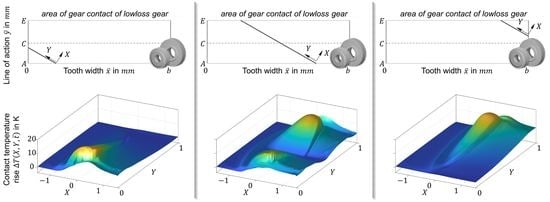
First, the tribological quantities such as hydrodynamic, solid and total contact pressure as well as the lubricant film thickness and contact temperature rise are explained along selected contact lines. Second, the frictional power and its local characteristics are analyzed, followed by an analysis of thermal effects.

For each time step of gear mesh, the results of the thermal EHL simulation can be shown along the contact line. For simplification, a dimensionless time $\overline{t}=t/t_c$ is chosen. The presentation of results concentrates on three characteristic time steps ${\overline{t}}_1$, ${\overline{t}}_2$ and ${\overline{t}}_3$ at $10\%$, $50\%$ and $90\%$ of the total contact time $t_c$ as shown in Figure 9. The gear faces are at $\overline{y}=\left\{0;b\right\}$, the beginning of tooth mesh is at $\overline{x}=A$ and the end of tooth mesh is at $\overline{x}=E$.

3.1. Tribological Quantities along the Contact Line

Figure 10 shows the calculated hydrodynamic pressure $p_f$ (a), solid contact pressure $p_s$ (b), total pressure $p$ (c), lubricant film thickness $h$ (d) and contact temperature rise $\Delta T$ (e) for the three considered time steps ${\overline{t}}_1$, ${\overline{t}}_2$ and ${\overline{t}}_3$ of the gear mesh. For the hydrodynamic pressure $p\left(X,Y,\overline{t}\right)$, some specific characteristics can be identified. The crowning of the gear tooth in the face width direction (see Figure 2f) causes a drop in the hydrodynamic pressure at the gear faces. Therefore, the hydrodynamic pressure slowly reduces at ${\overline{t}}_1$ in the positive $Y$-direction and at ${\overline{t}}_3$ in the negative $Y$-direction. In general, the contact shape changes from a more line-shaped contact at ${\overline{t}}_1$ to a more point-like contact at ${\overline{t}}_2$ to a more line-shaped contact at ${\overline{t}}_3$. There are pressure maxima in the beginning (A) and end of the gear mesh (E), which is typical for finite line contacts as analyzed by Habchi [23]. The center section at ${\overline{t}}_2$ shows an elliptical pressure distribution typical for point contacts.

The solid contact pressure $p_s\left(X,Y,\overline{t}\right)$ directly results from the lubricant film thickness $h\left(X,Y,\overline{t}\right)$ and the solid contact pressure curve $p_s\left(h\right)$ in Figure 6. A decrease in lubricant film thickness leads to a significant increase in solid contact pressure. However, the solid contact pressure is comparatively low at the gear face edges at $Y=1$ at ${\overline{t}}_1$ and $Y=0$ at ${\overline{t}}_3$. In the central area of the contact lines, the solid contact pressure is moderate and plateau-like. The drop of the hydrodynamic pressure at the beginning and end of the gear mesh leads to a drop in the lubricant film thickness, which again locally increases the solid contact pressure. The total pressure $p\left(X,Y,\overline{t}\right)$ represents the combination of the hydrodynamic pressure $p_f\left(X,Y,\overline{t}\right)$ and the solid contact pressure $p_s\left(X,Y,\overline{t}\right)$.

The lubricant film thickness $h\left(X,Y,\overline{t}\right)$ is in accordance with the hydrodynamic pressure. For all time steps, a typical plateau is formed. The contour depends on the hydrodynamic pressure. A typical constriction in the X-direction at the end of the contact zone can be observed. At ${\overline{t}}_2$, a characteristic horseshoe-shaped film thickness contour can be noticed. At the edges of contact lines at $Y=\left\{0;1\right\}$, a constriction with minimum lubricant film thickness is formed. Even at the edges with a continuous hydrodynamic pressure drop (${\overline{t}}_1$ at $Y=1$; ${\overline{t}}_3$ at $Y=0$), a constriction can be noticed after a moderate increase in the film thickness. This is to be expected for finite line contacts with straight roller geometry and the considered boundary conditions (Section 2.3, Habchi [23]).

The contact temperature rise $\mathsf{\Delta }T\left(X,Y,\overline{t}\right)$ is related to the heat sources by lubricant shearing and compression and solid friction. Characteristics for a thermal EHL contact such as the rise in temperature with pressure increase, a temperature drop after the pressure maximum, followed by a temperature tail can be seen. For the time steps ${\overline{t}}_1$ and ${\overline{t}}_3,$ the contact line does not cross the pitch point C with pure rolling ($SRR=0)$. Due to the increasing sliding velocity in the direction of the higher hydrodynamic pressure in $Y$-direction, a strongly asymmetric temperature profile is established with high temperatures at the edges. At time step ${\overline{t}}_2,$ the influence of the sliding velocity on the temperature change becomes clear. At the pitch point C with pure rolling, there is only a minimal increase in temperature. As the distance to the pitch point increases, the contact temperature strongly increases, which is consistent with the increase in sliding. In comparison to conventional gear designs, the overall contact temperature rise for the low-loss gear is very small. Ziegltrum et al. [24] shows for a more conventional gear design and similar operating conditions temperature rises of up to $50\mathrm{K}$.

3.2. Tribological Quantities across the Area of Gear Contact

Figure 11 gives a fuller picture over the EHL calculation results by plotting tribological quantities across the area of gear contact. Each quantity is evaluated and plotted along 250 contact lines which lie diagonal in the area of gear contact (see Figure 2). Figure 11a shows the line load $f_N\left(\overline{x},\overline{y}\right)$ along the contact lines considering the total contact load. It is determined by first integrating the total contact pressure $p\left(X,Y,\overline{t}\right)$ along the x-direction of the EHL contact for each time step (see Figure 10), before it is mapped into the area of gear contact $f_N\left(\overline{x},\overline{y}\right)$. The maximum of the total pressure $p_{}\left(X,Y,\overline{t}\right)$, hydrodynamic pressure $p_f\left(X,Y,\overline{t}\right)$, solid contact pressure $p_s\left(X,Y,\overline{t}\right)$, contact temperature rise $\mathsf{\Delta }T\left(X,Y,\overline{t}\right)$ and shear stress $\tau \left(X,Y,\overline{t}\right)$ in Figure 11b–e are evaluated along the x-direction of the EHL contact for every evaluated point in the y-direction and for each time step and mapped onto the area of gear contact $f_N\left(\overline{x},\overline{y}\right)$. Thereby, $\mathsf{\Delta }{T}_{max}\left(X,Y,\overline{t}\right)$ and ${\tau }_{f,max}\left(X,Y,\overline{t}\right)$ are evaluated at $z=h/2$. Considering the discrete evaluation of the quantities across the area of gear contact, the plots in Figure 11 show some unevenness.

The line load $f_N\left(\overline{x},\overline{y}\right)$ in Figure 11a is driven by the total contact load. The geometrical effect of crowning of the gear teeth (see Figure 2f) in the tooth width direction is clearly visible. Towards the beginning and end of the gear mesh, there is a decline in the load. Although the hydrodynamic load drops to zero here, the solid contact pressure (see Figure 11d) leads to an increase in the line load again, especially at these edges. This can also be seen in the distribution of the maximum hydrodynamic $p_{max}{}_{}\left(\overline{x},\overline{y}\right)$ and solid contact pressure $p_{s,max}\left(\overline{x},\overline{y}\right)$ in Figure 11c,d. The hydrodynamic pressure dominates the line load in the majority of the area of gear contact. There is a strong increase in the solid contact pressure only at the beginning and end of the gear mesh. As expected, the shear stress of the lubricant ${\tau }_{f,max}\left(\overline{x},\overline{y}\right)$ is related to the hydrodynamic pressure. The pitch point C is visible, where the sliding velocity and shear stress tend to zero. The influence of the pitch point can also be seen in the maximum contact temperature rise $\mathsf{\Delta }{T}_{max}\left(\overline{x},\overline{y}\right)$. With increasing the sliding velocity with distance from the pitch point C, the maximum contact temperature rises strongly.

3.3. Frictional Power Density

In the following, the power dissipation is investigated in detail. Besides frictional power loss by shearing or compression of oil, the solid contacts results in solid friction and thus frictional power loss. In order to understand the influences across the area of gear contact, the local friction power density $d{P}_F/dA$ is calculated:

$$\begin{array}{c}\frac{d{P}_{L,f}}{dA}={\tau }_{f,zx}\cdot \left|v_{1x}-v_{2x}\right|\\ \frac{d{P}_{L,s}}{dA}={\tau }_s\cdot \left|v_{1x}-v_{2x}\right|\end{array}\}atz=h/2$$

(21)

As Equation (21) shows, the power loss density depends linearly on the velocity difference $\left|v_{1x}-v_{2x}\right|$. It is zero at the pitch point C, which is also represented in the calculated power loss densities $d{P}_{F,f}/dA$, $d{P}_{F,s}/dA$ and $d{P}_F/dA$ at time step ${\overline{t}}_2$ shown in Figure 12a–c. At time step ${\overline{t}}_1$ and ${\overline{t}}_3$, the pitch point C is not on the contact line. When comparing the frictional power densities, it can be seen that $d{P}_{F,f}/dA$ dominates in most of the contact areas and represents the largest proportion. Towards the edge the shear stress decreases, which leads to a drop in the fluid friction. At the edges at $Y=1$ and $Y=0$, there is a rapid increase in the solid frictional power density $d{P}_{F,s}/dA$, in accordance with the solid contact pressure in Figure 10, but with the linear influence of the sliding velocity. The proportion of $d{P}_{F,s}/dA$ in the central mixed friction region of the contact line is subordinated. By comparing the total frictional power density $d{P}_F/dA$ with the temperature distribution in Figure 10, clear parallels can be seen and the individual heat sources can be identified.

3.4. Analysis of Thermal Effects

The presented calculation results relate to the EHL simulation considering non-Newtonian, thermal effects and mixed lubrication. Hence, the influence of thermal effects on the power loss densities are included. In order to quantify the influence of these thermal effects, a comparison of the power loss calculation in Section 3.2. with an isothermal EHL simulation is made, using an identical model apart from the thermal part.

Figure 13 shows the calculated frictional power densities $d{P}_{L,f}/dA$, $d{P}_{F,s}/dA$ and $d{P}_F/dA$ at time steps ${\overline{t}}_1$, ${\overline{t}}_2$ and ${\overline{t}}_3$ for the isothermal EHL simulation. In comparison with the thermal EHL simulation results in Figure 12, $d{P}_{L,s}/dA$ remains nearly unchanged, whereas the fluid frictional power density $d{P}_{L,f}/dA$ increases. This becomes clearer in Figure 14, which shows the maximum fluid power density $d{P}_{L,f}/dA$ (a), the fluid friction power loss $P_{L,f}$ (b), the solid friction power loss $P_{L,s}$ (c) and the total fluid friction power loss $P_L$ (d) for the isothermal and thermal EHL calculation along the dimensionless contact time. Thereby, the power loss densities $d{P}_{L,i}/dA$ are integrated over the contact area.

The maximum fluid frictional power density $d{P}_{L,f}/dA$ from the thermal EHL calculation is maximal $34.7\%$ lower compared the isothermal EHL calculation, whereas the fluid frictional power $P_{L,f}$ is maximal $17.7\%$ lower. The solid frictional power $P_{L,s}$ is maximal $7.7\%$ higher. This results in a total frictional power loss $P_L$, which is only maximal $9.4\%$ lower for the thermal EHL compared to the isothermal EHL calculation.

The reduction in the fluid frictional power density $d{P}_{L,f}/dA$ is due to thermal effects. The heat sources in the thermal EHL contact leads to an increase in temperature, which in return leads to a decrease in the effective contact viscosity and thus to a reduction in fluid friction. This effect is well known and pronounced for DLC coatings ([22,45]). At positions across the area of gear contact with a high load and sliding, the reduction in $d{P}_{L,f}/dA$ is highest. As $d{P}_{L,f}/dA$ is a very local value, the reduction in the fluid frictional power $P_{L,f}$ along the gear mesh is smaller. The solid frictional power $P_{L,s}$ is hardly influenced and even increases slightly, as the film thickness is governed by the conditions at the contact inlet of EHL contacts. There, the influence of the contact temperature increase is comparably small. Accordingly, the reduction in the total frictional power $P_L$ is mainly governed by the reduction in $P_{L,f}$.

The small differences between the thermal and isothermal EHL calculation at the considered operating condition show that the effect of thermal reduction in gear friction is small for low-loss gears. This is consistent with the experimental results of Hinterstoißer et al. [7], who shows that the thermal reduction in the load-dependent gear power loss is less pronounced for low-loss compared to conventional gear geometries.

4. Conclusions

This study analyzed the tribological behavior of a low-loss gear geometry using a transient EHL model considering thermal effects and mixed lubrication. Special focus was placed on local frictional losses to analyze the role of the thermal effects of the gear mesh. The main conclusions are:

• The EHL contact of low-loss gears is determined by a short path of contact with resulting small sliding portions;
• The edge geometry has a strong influence on lubricant film thickness and frictional power losses;
• The frictional power density obtained from the numerical calculation can be used to characterize the specific power input to fluid and solids;
• The thermal reduction in fluid friction is observed at gear mesh positions with a high load and sliding;
• Due to small sliding portions across the gear mesh, the general effect of the thermal friction reduction is small.

Low-loss gears are an interesting design approach for increasing gearbox efficiency and thermal load limits, e.g., for dry or minimum quantity lubrication. The tribological comparison of low-loss gears with conventional gear geometries and the validation of calculation results with power loss measurements can be the focus of further investigations.