Steady-State Temperature Field and Rolling Resistance Characteristics of Low-Speed and Low-Load Capacity Non-Pneumatic Tires

Abstract

Rolling resistance (RR) is key research content for developing low-carbon energy-saving tires, and the resultant change in the tire temperature field exerts a crucial impact on tire performance. Currently, there is no accurate and systematic analysis method for solving the steady-state temperature field (SSTF) and RR of tires with complex patterns and non-pneumatic tires (NPTs), which are characterized by discontinuous structure in the circumferential direction. A solution strategy that entails SSTF and RR based on explicit transient rolling analysis and thermal-mechanical coupling is proposed and its accuracy is verified using the SSTF test pertaining to the low-speed and low-load capacity non-pneumatic tire (LSL-tire), which exhibits a 7.56% and 6.94% average temperature deviation for the outer surface center of the tread and for the outer surface center of spokes, respectively. Uniaxial tensile mechanical property tests and dynamic mechanical analysis (DMA) of the utilized rubber and polyurethane (PU) materials were conducted, and their specific heat capacity, thermal conductivity, and density were tested. Based on three-dimensional nonlinear finite element simulation and considering the characteristics pertaining to the loss factor of viscoelastic materials changing with temperature, the SSTF and RR of the LSL-tire under different loads and velocities were analyzed. The results indicate that the influence of load and speed on the SSTF of LSL-tire is quite significant, whereas the influence of speed on the RR is not apparent. For all conditions, the highest steady-state temperature points of the tread are located in its center, and in the spokes they are located in the joint between spokes and the outer ring; the spokes contribute the most to the RR, followed by the tread.

1. Introduction

Rubber or PU (for NPTs), the main component of tires, is a typical viscoelastic material that produces energy loss during deformation. The external work stored in the loading process cannot be completely released when unloaded, and part of the energy is utilized to overcome the friction inside the material, which is manifested as heat; thus, the tire is heated or heat is dissipated to the environment. Moreover, the resultant temperature rise in the tire will affect its material properties, which in turn affects the service life of the tire. Thus, RR is a key parameter in the tire design process.

For a 10% reduction in RR, the fuel economy of light trucks and passenger cars should be increased by 0.5% to 1.5%, and by 1.5% to 3% for heavy trucks [1]. For pure electric vehicles, due to the existence of the battery, their body weight is 10% to 20% heavier than that of fuel vehicles, and the energy utilization efficiency of the vehicles’ power and transmission system is relatively enhanced; therefore, reducing tire RR is a more effective method of enhancing their mileage. Transportation vehicles contribute approximately 58% of oil consumption and 20% of greenhouse gas emissions worldwide [2]; therefore, low RR tire technology is crucial research content for the development of green vehicles. Many scholars have performed valuable studies on the RR or SSTF of tires using the finite element (FE) method. Based on whether the energy dissipation algorithm of viscoelastic materials encapsulated by FE commercial software is adopted, it can be divided into the following two categories.

The first method includes three modules, namely the deformation module, the energy dissipation module, and the heat transfer module. Scholars have exhibited different opinions on the aforementioned three modules. Shida et al. [3] analyzed the RR of radial tires based on static FE analysis. The stress and strain of all elements along the circumferential direction corresponding to a certain element on a cross section are regarded as the stress and strain cycle when the element rolls for a revolution. Furthermore, the homogenization method [4] is utilized to obtain the equivalent loss tangent of the anisotropic rubber-based composite materials. Hall et al. [1] utilized the principal stress, principal strain, and loss modulus, which are influenced by temperature, strain amplitude, and frequency, to calculate the hysteresis energy and heat generation rates. Lin et al. [5] utilized the ratio of the loss modulus to the complex modulus as the hysteresis factor, and the hysteresis energy loss was expressed as a function of the hysteresis factor and strain energy. Tang et al. [6] utilized the steady-state transport (SST) function of Abaqus simulating the free rolling state of the tire to obtain the elastic strain energy. The hysteresis energy algorithm is similar to the study conducted by Lin. Li et al. [7], who utilized the linear interpolation method and the modified Kraus model [8] to express the loss modulus. Moreover, the deformation analysis was based on the implicit environment. Convective heat transfer coefficients between the solid tire’s surfaces and air were determined based on references [9,10]. He et al. [11] continued to explore the study conducted by [7] using the co-simulation method based on Abaqus and Endurica. Based on the Lagrangian model, the Lagrangian–Eulerian model, and the plane strain model, which both exist in an implicit environment, the RR and temperature field are analyzed. Ding et al. [12] developed a tire–pavement interaction model in which the asphalt pavement’s thicknesses and moduli were set with different values to analyze the tire’s RR. Park et al. [13] proposed a novel simulation methodology for which Abaqus user subroutine UHYPEL was utilized to embed strain–stress–temperature curves to characterize the thermomechanical properties of cap ply. Cho et al. [14,15] and LEE et al. [16] established a 3D full-patterned tire model with two different patterns and performed a static contact analysis. Furthermore, the strain cycles of each element in one sector during a revolution are estimated by determining the stress of elements at the same position in the circumferential direction. Fu et al. [17] converted the six-dimensional stress and strain into equivalent stress and strain to calculate the heat generation rate, and they analyzed the SSTF of NPTs based on the implicit environment. Marin et al. [18] analyzed the boundary and initial conditions in the thermoelasticity theory for micropolar materials with pores, and they obtained some results regarding the existence and uniqueness of a finite energy solution.

The second method utilizes the ALLCD (energy dissipated by viscoelasticity, creep, and swelling) in the post-processing energy outputs of the FE commercial software Abaqus2018 as the hysteresis energy loss. Kim et al. [19] utilized Maxell models to construct viscoelastic constitutive equations, which are expressed as a Prony series. The rolling stroke of the NPT along the forward direction is set at 1 m and the obtained ALLCD is the hysteresis energy loss generated when the tire travels per unit distance (i.e., the RR of the tire). Yoo et al. [20,21] also utilized the aforementioned method to calculate the hysteresis energy loss of NPTs with lattice spokes, for which the spokes and shear band are divided into several subcomponent sets. For the thermal analysis, the average heat generation rate of each subcomponent set is utilized as the heat generation rate of each element. Moreover, Jin et al. [22] utilized a similar method to calculate the hysteresis energy loss, and the RR of three categories of NPTs with different support structures are analyzed. Veeramurthy et al. [23,24,25] utilized the Prony series to represent the linear viscoelastic behavior of materials, and the RR of NPTs were analyzed based on the 2D plane strain model. Aldhufairi et al. [26,27] utilized the parallel rheological framework and the Prony series to characterize the viscoelasticity. Kiran et al. [28] analyzed the influence of three categories of hyperelastic constitutive models on the RR of NPTs.

Currently, the simulation technology pertaining to the SSTF and RR of pneumatic tires can basically satisfy industrial application requirements. Applying the symmetric model generation (SMG) capability and SST analysis to complete the 3D modeling and free rolling simulation of pneumatic tires is a typical simulation method that is widely applied. However, SST analysis exhibits some limitations. It requires the following: the 3D model generated using a 2D cross-section or a single 3D sector through SMG capability should exhibit continuous streamlines which regulate the motion of the material, and the chosen repetitive angle segment must be small enough to ensure that the material convection is accurate. Moreover, the correlation between the friction stress and the deformation history of the circumferential discontinuous structure of the tire on the contact surface is ignored. Therefore, for solving the SSTF and RR of tires with complex patterns and NPTs (whose typical characteristics are discontinuous in the circumferential direction) using SST analysis, theoretical error exists.

Herein, a novel strategy for solving the SSTF and RR of NPTs based on explicit dynamic analysis and considering the loss factor of viscoelastic materials, which varies with temperature, is proposed. Moreover, the strategy, which is not only applicable to tires, can also be theoretically be applied to any object composed of viscoelastic materials, and the strategy does not assume that the steady-state temperature of each radial cross-section of the tire is the same. The main contents of the paper include the LSL-tire structure, SSTF experiment, material experiment, hysteresis theory of viscoelastic material, heat generation rate and RR algorithm of NPTs, and FE simulation of transient rolling and heat transfer. Furthermore, the accuracy of the FE simulation is verified. The SSTF and RR of the LSL-tire under different loading and velocity conditions are analyzed and discussed in detail.

2. Research Method

2.1. Structure of the LSL-Tire

The design velocity and rated load of the LSL-tire are 25 km/h [29,30] and 735 N [31], respectively. The LSL-tire is composed of a tread, shear band, outer ring, inner ring, and 40 spokes which are arranged along the circumference. The outer diameter of the LSL-tire is 252 mm, and the thicknesses of the spoke, outer ring, and inner ring are 2 mm, 2 mm, and 5 mm, respectively (Figure 1a). The tread width, tread thickness, and shear band thickness of the LSL-tire are 60 mm, 19 mm, and 13 mm, respectively. The diameter of the glass fiber in the shear band is 2.3 mm. There are 12 glass fibers in Enhancement Layer 1, 13 glass fibers in Enhancement Layer 2, and 18 glass fibers in Enhancement Layer 3 (Figure 1b).

The shear band of the LSL-tire crucially enhances the stiffness of the tread. The tread stiffness design can be achieved by changing the type and thickness of the rubber between the reinforcement layers and the type and geometric parameters of the reinforcement material. The spoke crucially affects the bearing, and its stiffness can also be designed by changing the geometric parameters and material types. The decoupling design pertaining to the overall stiffness and grounding characteristics of the LSL-tire can be realized by designing the stiffness of the tread and the spoke, respectively.

The material utilized in the tread and shear band of the LSL-tire is the same kind of vulcanized natural rubber compound, which is formed by the vulcanization process after preforming. The outer ring, inner ring, and spokes are composed of the same kind of polyurethane, which are formed by an injection molding process. Finally, the inner surface of the tread and the outer surface of the outer ring are bonded together by a special adhesive; thus, the sample tire is obtained.

2.2. Hysteresis Effect of Viscoelastic Materials

When the viscoelastic material which exhibits hysteresis characteristics is deformed under loading, it should overcome its internal friction, which will occasion a scenario in which the strain lags behind the stress, resulting in hysteresis energy loss. The viscoelastic material element is subjected to uniaxial sinusoidal strain [1] as depicted in Figure 2a:

$$\epsilon \left(\theta \right)={\epsilon }_0·sin\theta$$

(1)

where ${\epsilon }_0$ denotes the strain amplitude, and $\theta$ denotes the loading phase. The corresponding sinusoidal stress is obtained as follows [1]:

$$\sigma \left(\theta \right)={\sigma }_0·sin(\theta +\delta )$$

(2)

where ${\sigma }_0$ denotes the stress amplitude, and $\delta$ denotes the lag angle. The stress and strain are integrated in a loading period [1]:

$$h={\int }_0^{\theta }\sigma \left(\theta \right)d\epsilon \left(\theta \right)=\pi ·{\epsilon }_0·{\sigma }_0·sin\delta$$

(3)

The hysteresis energy loss density $h$ per unit volume of the material, (i.e., the area of the hysteresis loop), is obtained, as illustrated in Figure 2b.

The storage modulus $E^{\prime }$ of viscoelastic materials is defined as the ratio of stress to strain amplitude in the same phase [13]:

$$E^{\prime }=\frac{{\sigma }_0}{{\epsilon }_0}·\mathit{cos}\delta$$

(4)

The loss modulus $E^{″}$ is defined as the ratio of stress to strain amplitude with a phase angle difference of 90 degrees [13]:

$$E^{″}=\frac{{\sigma }_0}{{\epsilon }_0}·sin\delta$$

(5)

The loss factor is defined as the ratio of loss modulus to storage modulus [13]:

$$tan\delta =\frac{E^{″}}{E^{\prime }}$$

(6)

where $E^{\prime }$, $E^{″}$ and $tan\delta$ are obtained using DMA. There is a complex nonlinear relationship between the loss factor of the viscoelastic material and its loading frequency, strain amplitude, and temperature. Herein, it is simplified to consider only the nonlinear relationship between the loss factor and temperature at a certain loading frequency.

2.3. Rolling Resistance of the LSL-Tire

The RR of tires is defined as the energy loss when the tire travels per unit distance. The energy loss of the tire during rolling is occasioned by three aspects: the hysteresis loss of the tire material, the friction energy loss between the tread and the ground, and the air resistance to the tire. The hysteresis loss accounts for more than 90%; therefore, we ignore the other two energy losses.

During the rolling process of the tire, the material elements of rubber and polyurethane are in a complex six-directional stress state, and the solution of the hysteresis energy loss density described in the upper section is applicable to only the uniaxial harmonic stress state. Therefore, the six-directional stress and strain are converted into equivalent stress and strain [32]:

$${\epsilon }_e=\frac{\sqrt{2}}{3}·\sqrt{{({\epsilon }_x-{\epsilon }_y)}^2+{({\epsilon }_y-{\epsilon }_z)}^2+{({\epsilon }_x-{\epsilon }_z)}^2+6({\epsilon }_{xy}^2+{\epsilon }_{yz}^2+{\epsilon }_{xz}^2)}$$

(7)

$${\sigma }_e=\frac{1}{\sqrt{2}}·\sqrt{{({\sigma }_x-{\sigma }_y)}^2+{({\sigma }_y-{\sigma }_z)}^2+{({\sigma }_x-{\sigma }_z)}^2+6({\sigma }_{xy}^2+{\sigma }_{yz}^2+{\sigma }_{xz}^2)}$$

(8)

where ${\epsilon }_e$ and ${\sigma }_e$ denote equivalent strain and equivalent stress, respectively, which are fitted as a harmonic function by the Fourier series [12]:

$${\epsilon }_e\left(t\right)=a_0^{\epsilon }+\sum _{n=1}^N\left[a_n^{\epsilon }·cos\left(n\omega t\right)+b_n^{\epsilon }·\mathit{sin}\left(n\omega t\right)\right]$$

(9)

$${\sigma }_e\left(t\right)=a_0^{\sigma }+\sum _{n=1}^N\left[a_n^{\sigma }·\mathit{cos}\left(n\omega t\right)+b_n^{\sigma }·\mathit{sin}\left(n\omega t\right)\right]$$

(10)

where $N$ denotes the order of the Fourier series, and accurate fitting can be achieved when $N$ is 26. Furthermore, taking the equivalent stress of an element in the spoke center extracted from the finite element analysis results in Section 3, as an example, the fitting effect is depicted in Figure 3. $a_0$ denotes the Fourier coefficient, $\omega$ denotes the rolling angular velocity of the tire, $a_n$ and $b_n$ denote the amplitudes of the string function, and $t$ denotes the rolling time. Equations (9) and (10) are expressed as sine functions using the auxiliary angle formula [33]:

$${\epsilon }_e\left(t\right)=a_0^{\epsilon }+\sum _{n=1}^N[A_n^{\epsilon }·\mathit{sin}(n\omega t+{\phi }_n^{\epsilon }\left)\right]$$

(11)

$${\sigma }_e\left(t\right)=a_0^{\sigma }+\sum _{n=1}^N[A_n^{\sigma }·\mathit{sin}(n\omega t+{\phi }_n^{\sigma }\left)\right]$$

(12)

where $A_n=\sqrt{a_n^2+b_n^2}$, ${\phi }_n=\mathit{arctan}\left(\frac{a_n}{b_n}\right)$. The lagging angle of the viscoelastic material is added to the phase of equivalent stress [33]:

$${\sigma }_e\left(t\right)=a_0^{\sigma }+\sum _{n=1}^N[A_n^{\sigma }·\mathit{sin}(n\omega t+{\phi }_n^{\sigma }+\delta \left)\right]$$

(13)

The equivalent stress and strain of each viscoelastic material element are integrated in a single rolling period of the tire, and the hysteresis energy loss density of the element is obtained [33]:

$$h_e={\int }_0^{\raisebox{1ex}{$2\pi $}\!\left/ \!\raisebox{-1ex}{$\omega $}\right.}{\sigma }_e\left(t\right)d{\epsilon }_e\left(t\right)=\sum _{n=1}^N[n·\pi ·A_n^{\epsilon }·A_n^{\sigma }·\mathit{sin}\left({\phi }_n^{\sigma }-{\phi }_n^{\epsilon }+\delta \right)]$$

(14)

The sum pertaining to the product of the hysteresis energy loss density of each viscoelastic material unit and unit volume is the whole hysteresis energy loss of the tire when it rolls one cycle [33]:

$$E_{loss}=\sum _{m=1}^{Nele}\sum _{n=1}^N[n·\pi ·V_m·A_{n,m}^{\epsilon }·A_{n,m}^{\sigma }·\mathit{sin}\left({\phi }_{n,m}^{\sigma }-{\phi }_{n,m}^{\epsilon }+{\delta }_m\right)]$$

(15)

where $m$ denotes the unit number, $V_m$ denotes the unit volume, and ${\delta }_m$ denotes the lag angle of the unit. When the tire attains the SSTF, the temperature of each unit is different, which results in different lag angles. The ratio of the hysteresis energy loss to the rolling distance during one rolling cycle is the RR of the tire [12]:

$$F_R=\frac{E_{loss}}{2\pi r}$$

(16)

where $r$ denotes the rolling radius of the tire.

2.4. Heat Generation Rate of Element

The hysteresis energy loss of the viscoelastic material is converted into heat; thus, the tire is heated. The heat generation rate of the element is obtained using the following formula [15]:

$$q_m=\frac{h_e}{T}=\frac{{\omega ·h}_e}{2\pi }$$

(17)

where $T$ denotes the rolling period of the tire. The temperature change of the tire during rolling affects the loss factor of the viscoelastic material, and, subsequently, affects the element heat generation rate until the tire attains the SSTF. The thermal–mechanical coupling FM analysis process of the LSL-tire is illustrated in Figure 4.

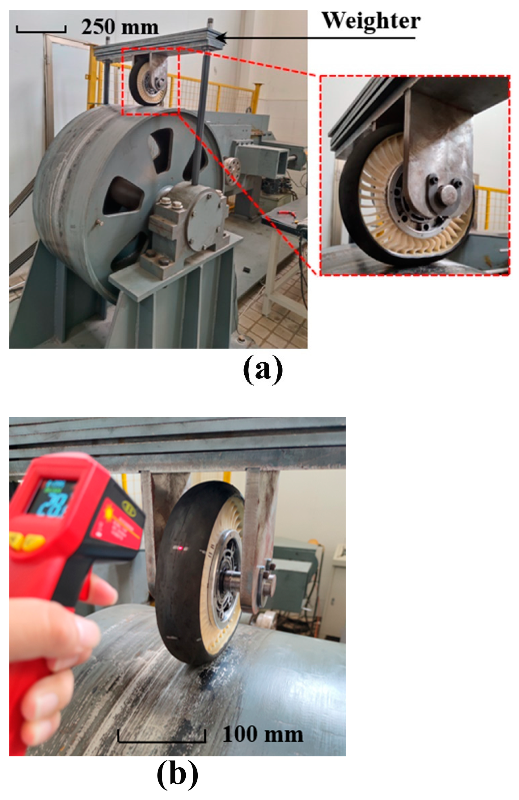
2.5. Steady-State Temperature Field Test of the LSL-Tire

The LSL-tire was assembled with the hub and parked at the test site for at least 3 h, before each test, to achieve thermal balance at ambient temperature. As depicted in Figure 5a, the LSL-tire was installed on the test bench to test at a 25 km/h speed under a 520 N load until it attained the SSTF. Three temperature measurement points were marked on the surface center of the tread and the surface center of spokes of the LSL-tire along the circumference (Figure 5b), and the DTM-S1 non-contact infrared thermometer was utilized to measure the temperature immediately after each test.

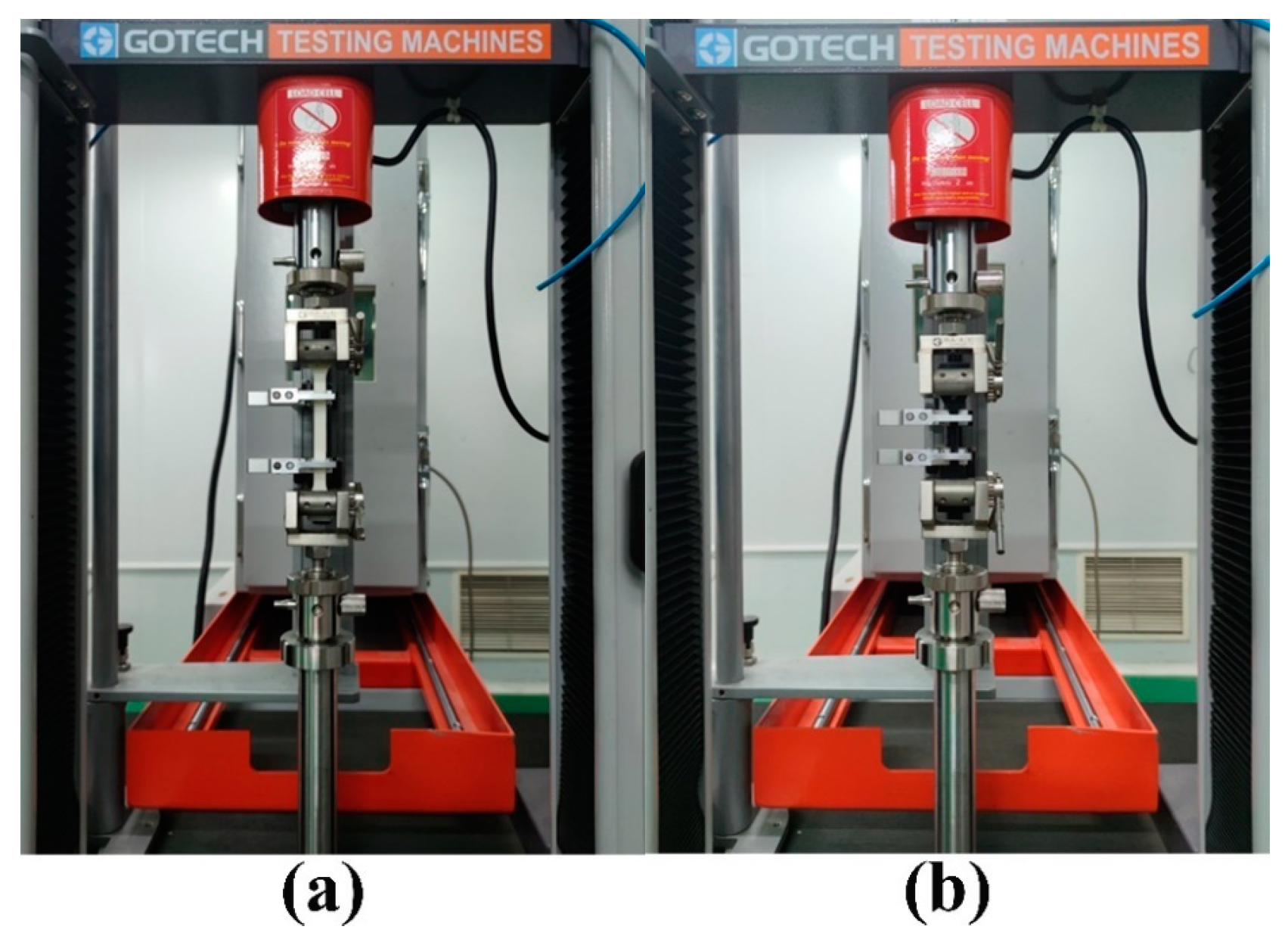
2.6. Mechanical Properties Test of Materials

The material utilized for the LSL-tire tread is rubber, and the material utilized for its outer ring, spokes, and inner ring is polyurethane (PU). According to GB/T 1040.2-2022 [34] and GB/T 528-2009 [35], three dumbbell-shaped uniaxial tensile specimens of PU and rubber were cut, and the uniaxial tensile mechanical properties were tested at the tensile speeds of 50 mm/min and 500 mm/min as shown in Figure 6a and Figure 6b, respectively.

2.7. Thermodynamic Parameters and Density Test of Materials

According to GB/T 40396-2021 [36], two DMA tensile specimens of rubber and polyurethane were cut. The dynamic mechanical analysis of the specimens under tensile mode was performed using GABO EPLEXOR thermomechanical analyzer in the temperature range of −20 °C to 100 °C with a loading frequency of 10 Hz and a temperature rise rate of 1 °C/min (Figure 7a).

According to GB/T 19466.4-2016 [37], the solid particles of rubber and PU were utilized as samples, and the DSC25 differential scanning calorimeter was utilized to continuously scan them in the 0 °C to 50 °C temperature range (Figure 7b).

According to GB/T 22588-2008 [38], the thermal conductivity test samples of PU and rubber were cut and tested using a XIATECH TC3000E thermal conductivity meter. The densities were measured using a Byes-300c automatic electronic densitometer.

2.8. Structural Deformation Analysis

The FE model of the LSL-tire is depicted in Figure 8. All the simulation analysis work herein was completed using the Abaqus FE software. The mechanical properties of rubber and PU were described using the Marlow constitutive whose strain energy potential form is expressed as follows:

$${\mathrm{U}}_{\mathsf{\epsilon }}={\mathrm{U}}_{\mathrm{dev}}\left({\stackrel{\mathrm{-}}{\mathrm{I}}}_1\right)+{\mathrm{U}}_{\mathrm{vol}}\left({\mathrm{J}}_{\mathrm{el}}\right)$$

(18)

where ${\mathrm{U}}_{\mathsf{\epsilon }}$ denotes the strain energy stored within a unit volume of the material: ${\mathrm{U}}_{\mathrm{vol}}$ denotes its volumetric component, and ${\mathrm{U}}_{\mathrm{dev}}$ denotes the deviatoric component. The first deviatoric strain invariant is ${\stackrel{\mathrm{-}}{\mathrm{I}}}_1$, and the elastic volume ratio is ${\mathrm{J}}_{\mathrm{el}}$. The reason for using this constitutive is described in the previous study [39]. The material constitutive models obtained by fitting the uniaxial tensile test data are illustrated in Figure 9. The transient rolling analysis of the LSL-tire was performed in the Dynamic/Explicit environment of Abaqus. The tread, shear band, outer ring, spokes, and inner ring were meshed using eight-node and six-node linear reduced integration elements, namely C3D8R and C3D6R. The glass fiber reinforced layers were characterized by rebar elements which are meshed using four-node reduced integration surface elements, namely SFM3D4R. And the whole model comprised 215,520 elements and 262,080 nodes.

The tread, outer ring, spokes, and inner ring were constrained together by common-node elements in the FE model. The nodes located on the inner surface of the inner ring and the reference point located on the geometric center of the LSL-tire were constrained together by a coupling mechanism. Furthermore, the rebar elements were embedded in the host elements. The drum of the rolling test bench which exhibits surface-to-surface contact with the tread is modeled using an analytical rigid surface. The contact property for which the normal and tangential behaviors were described using the hard and penalty algorithms. The friction coefficient between the drum and tread was set at 0.85. The whole analysis process included two ‘Dynamic, Explicit’ steps. In the first analysis step, six degrees of freedom of the tire reference point and five degrees of freedom of the drum reference point were constrained, and the latter was subjected to different displacements along the positive direction of the z-axis to apply different loads. In the second analysis step, the rotational degrees of freedom of the LSL-tire and the drum around the y-axis were released, and different angular velocities were applied to the drum to change the rolling speed of the LSL-tire.

After the explicit transient rolling analysis of the LSL-tire was completed, the stress and strain fields of all elements except rebar elements in a single rolling period of the LSL-tire were extracted from the result file, and the heat generation rate of all elements were calculated according to Formula (17). When the heat transfer analysis was completed and the LSL-tire attained the SSTF, the RR was calculated as per Formula (16).

2.9. Heat Transfer Analysis

In the proposed study, which differs from solving the temperature field of pneumatic tires based on the 2D FE model, we solved the SSTF based on the 3D FE model of the LSL-tire. Furthermore, eight-node heat transfer linear reduced integration brick elements DC3D8R and six-node linear heat transfer triangular prism elements DC3D6 were utilized. The air resistance, friction energy loss, thermal radiation, and hysteresis loss of glass fiber were not considered, and the hysteresis loss of the viscoelastic material was utilized as the only heat source input. The thermal conductivity, specific heat capacity, and density data utilized for the material properties of the FE model refer to the test data in

Table 1. Thermodynamic parameters and density of the material.

Material	Specific Heat Capacity (J/(g·°C))	Density (g/cm3)	Standard Deviation of Density	Thermal Conductivity (W/(m·k))	Standard Deviation of Thermal Conductivity
Rubber	1.476	1.206	0.12%	0.310	0.04714%
PU	1.805	1.135	0.16%	0.220	0

, and the ambient temperature and the initial temperature of the LSL-tire were set at 27.8 °C. All outer surfaces of the LSL-tire were subjected to convective heat transfer with air, and the convective heat transfer coefficient was determined as per the existing literature [18]. After the completion of the first heat transfer step analysis, the temperature pertaining to all elements of the LSL-tire changed, and the element heat generation rate was updated using Formula 17 according to the element temperature and the loss factor curves. Based on the modified LSL-tire temperature field and the updated element heat generation rates, the heat transfer analysis was performed again, and the analysis iterated until the temperature field of the LSL-tire attains a steady state. The judgment was rationalized as follows: the temperature fluctuation of all nodes of the LSL-tire was less than 1 °C.

3. Results and Discussion

3.1. Steady-State Temperature Field Results of the LSL-Tire

The average steady-state temperatures pertaining to the surface center of the tread and the surface center of spokes were 64.8 °C and 44.7 °C, respectively. During the rolling process of the LSL-tire, the FLIR-E64501 thermal imager was utilized to measure its temperature from the side, and the SSTF distribution is depicted in Section 3.4.

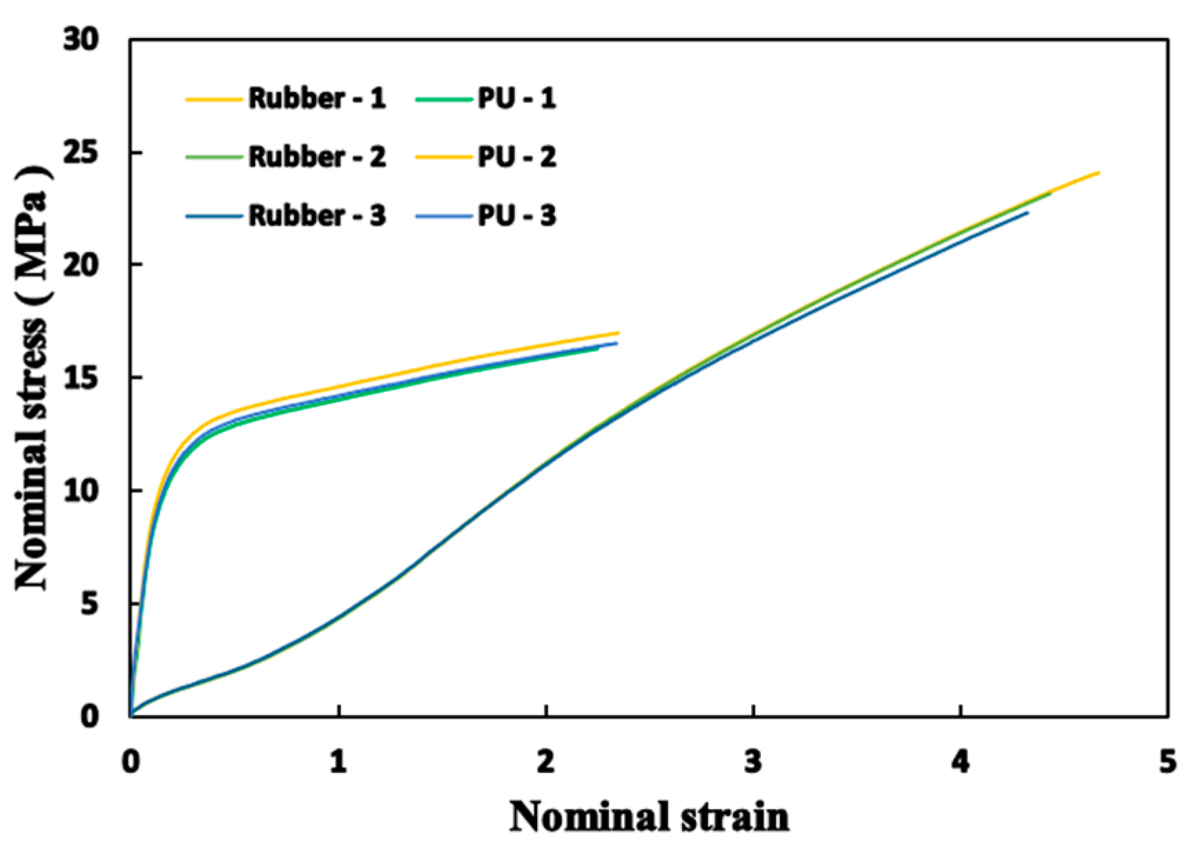
3.2. Mechanical Properties Results of Materials

The stress–strain test curves of rubber and PU are illustrated in Figure 10. It can be observed that the elongation at break of polyurethane was less than that of rubber, and its stress was significantly greater than that of rubber. The elastic modulus of the glass fiber was provided by its manufacturer as 35 GPa.

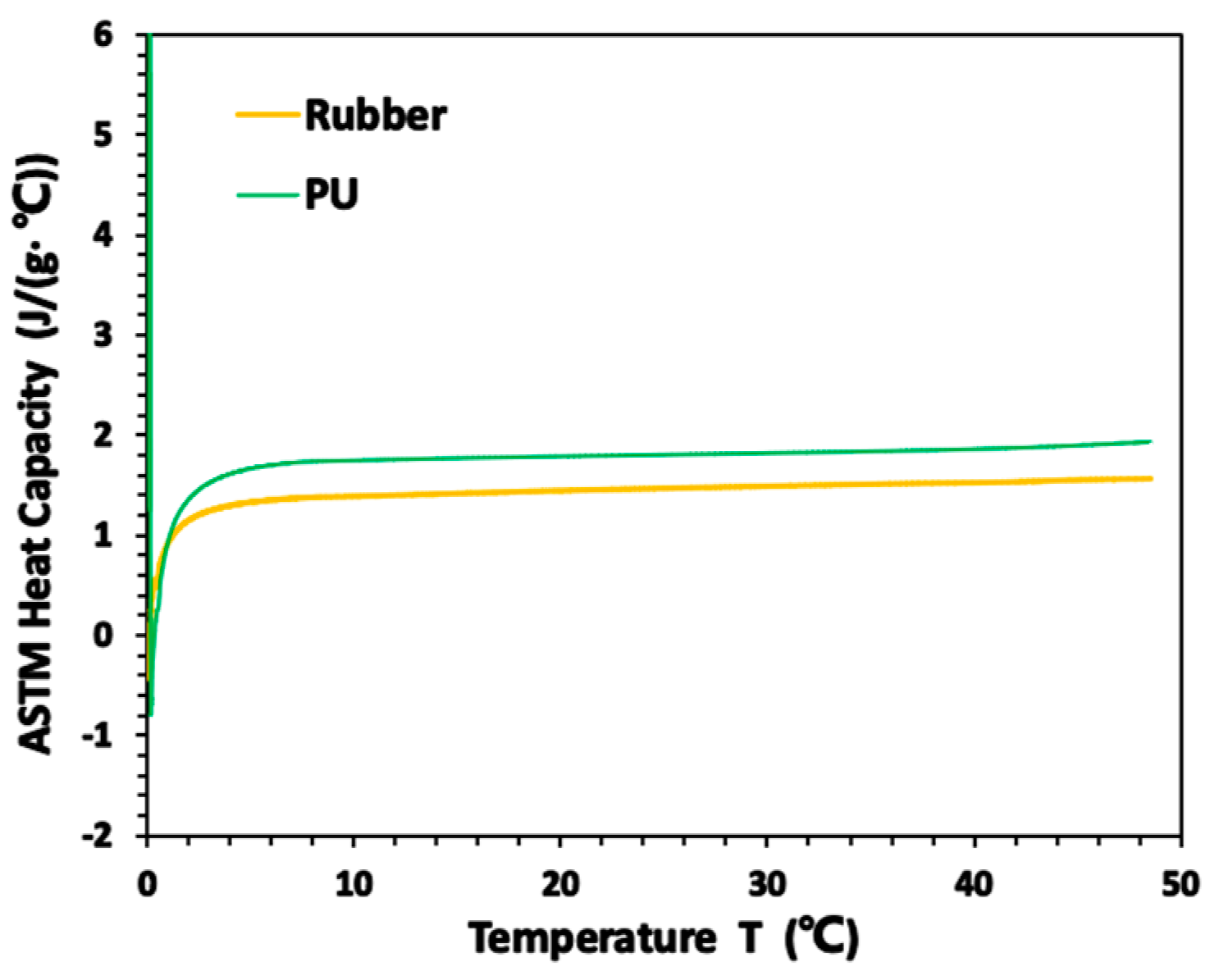
3.3. Thermodynamic Parameters and Density Results of Materials

The relationship curves pertaining to the storage modulus, loss modulus, and loss factor of rubber and PU with temperature are depicted in Figure 11a,b. It can be observed that the loss modulus and loss factor gradually tend to stabilize with the increase in temperature.

Curves pertaining to the specific heat capacity of the two materials with temperature are illustrated in Figure 12, which indicates that the fluctuation of the specific heat capacity with temperature is small. Table 1 indicates that the specific heat capacity data at 25 °C, which is 1.476 J/(g·°C) and 1.805 J/(g·°C) for the rubber and PU, respectively, can be utilized as the specific heat capacity value in the whole temperature range. The thermal conductivity and densities of the two materials are also depicted in Table 1; the density and its standard deviation are 1.206 (g/cm³) and 0.12% for the rubber and 1.135 (g/cm³) and 0.16% for the PU. Furthermore, the thermal conductivity and its standard deviation are 0.310 W/(m·k) and 0.04714% for the rubber and 0.220 W/(m·k) and 0 for the PU.

3.4. Validation of the FE Model

Four paths a, b, c, and d are established by selecting all the nodes of the tread outer surface center, the spoke outer surface center, the tread center, and the support center along the circumferential direction (Figure 13). The SSTF of the LSL-tire is simulated at a velocity of 25 km/h [37] under a load of 520 N [39], which is the most commonly utilized condition for the LSL-tire, and the temperature data of all nodes in paths a and b are extracted (Figure 14). It can be observed that the outer surface center temperature of the tread is between 55.9 °C and 64.3 °C, and its average temperature is 59.9 °C, which is a 7.56% departure from the experimental value (64.8 °C) whose standard deviation is 0.9031. The outer surface center temperature of the spokes is between 39.6 °C and 43.8 °C, and their average temperature is 41.6 °C, which is a 6.94% departure from the experimental value (44.7 °C) whose standard deviation is 0.6944. In the free rolling process of the LSL-tire, the circumferential discontinuity of the spokes leads to different stress states of each node located in the same path (a or b); therefore, each node exhibits different steady-state temperatures.

The cloud diagram and thermal imaging of the lateral SSTF of the LSL-tire are depicted in Figure 15. It can be observed that the distribution of the simulated temperature field is consistent with the real scenario. Among all the outer surfaces of the LSL-tire, the temperature of the tread is the highest, followed by the outer ring surface, the spoke surfaces, and the inner ring surface, in descending order. The temperature of the tread decreases from the middle to both sides along the direction of the tire width, and so does the temperature of the outer ring surface. The temperature of the spoke surfaces decreases from the middle to both sides along the radial direction; subsequently, it increases again. The temperature pertaining to the outer surface of the inner ring along the radial direction is higher than that of the inner surface. The relative error of the steady-state temperatures in the middle of the outer ring surface and in the middle of the outer surface of the inner ring are 6.91% and 8.19%, respectively. The highest thermal imaging temperature is 56.8 °C, and this observation is rationalized as follows: the shooting angle does not cover the surface center of the tread, which is the highest temperature point on the tread surface. Thus, the accuracy of the FE model is verified.

3.5. Steady-State Temperature Field and Rolling Resistance of the LSL-Tire under Different Loads

The SSTF of the LSL-tire was simulated and the RR was solved at the 25 km/h speed under the 294 N and 520 N load, respectively. The temperature field under each condition attains a steady state after two iterations. The iterative curves pertaining to the temperature of nodes in the four paths are illustrated in Figure 16, where the temperature distributions are apparently almost the same. It can be observed that the steady-state temperature of each part of the LSL-tire increases with the increase in load, because a higher load means larger stress and strain amplitudes, which caused higher $h_e$ and $q_m$. From Figure 16a, it can be observed that the temperature difference between the outer surface center of the tread and the center of the tread increases significantly with the load, and that the average steady-state temperature increases by 74.8% and 144.9% under the two conditions, respectively. It can be observed from Figure 16b that the temperature difference between the outer surface center of the spokes and the center of the spokes increases with the load, and that the average steady-state temperature increases by 10.1% and 29.5%, respectively, under the two conditions. It can be observed from Figure 17, the highest steady-state temperature points of the tread are located in the center of the tread, which are 77.7 °C and 171.1 °C, respectively; this phenomenon is different from that in which the highest steady-state temperature point of the tread is located at the belt edge for the pneumatic tire [14]. The distinction may be rationalized as follows: the tread structure of LSL-tire is different from that of a pneumatic tire. The tread of the LSL-tire is the thickest in the middle of the width direction, and the maximum equivalent stress of the tread appears at its center, which leads to a high heat generation rate and slow heat dissipation in the tread center. Moreover, the highest steady-state temperature points of the spokes are located in the center of the joint between spokes and the outer ring, which are 44.0 °C and 73.6 °C, respectively. This observation is due to the large heat generation rate at the aforementioned location. The heat of the tread and the outer ring will diffuse there, and because the thickness at the aforementioned location is larger compared to other positions of the spoke, the heat is not easily lost. Reference [19] also expounds that the temperature at the junction of the spokes and inner ring surface of the honeycomb structure NPTs is higher.

The contribution pertaining to the RR of each part of the LSL-tire under the two conditions is depicted in Figure 18a. It can be observed that the RR increases significantly with the load, which is consistent with the variation trend pertaining to the RR of the NPT that exhibits plane spokes with load in References [20,22]. The variation trend is occasioned by the increase in equivalent stress and strain amplitudes with the load, which leads to a scenario in which $h_e$ becomes larger with the load. The RR of the LSL-tire under the two conditions is 21.6 N and 75.2 N, respectively, and the growth rate is 248.1%. The spokes effected the highest impact on the RR, accounting for 56.5% and 62.9%, respectively, under the two conditions, followed by the tread, which accounted for 34.7% and 29.1%, respectively. Therefore, it has been confirmed that the design of the material and the geometry of the spoke are significantly crucial for reducing the RR. Figure 18b depicts the variation in RR with the total number of elements, where the detailed values of the four points are 80.0 N at 189,600, 76.3 N at 206,880, 75.2 N at 215,520, and 74.9 N at 226,320. It is confirmed that the mesh density taken for the FE analysis shows convergence in predicting the RR. Moreover, the number and size of the spoke elements exerts the greatest influence on the RR.

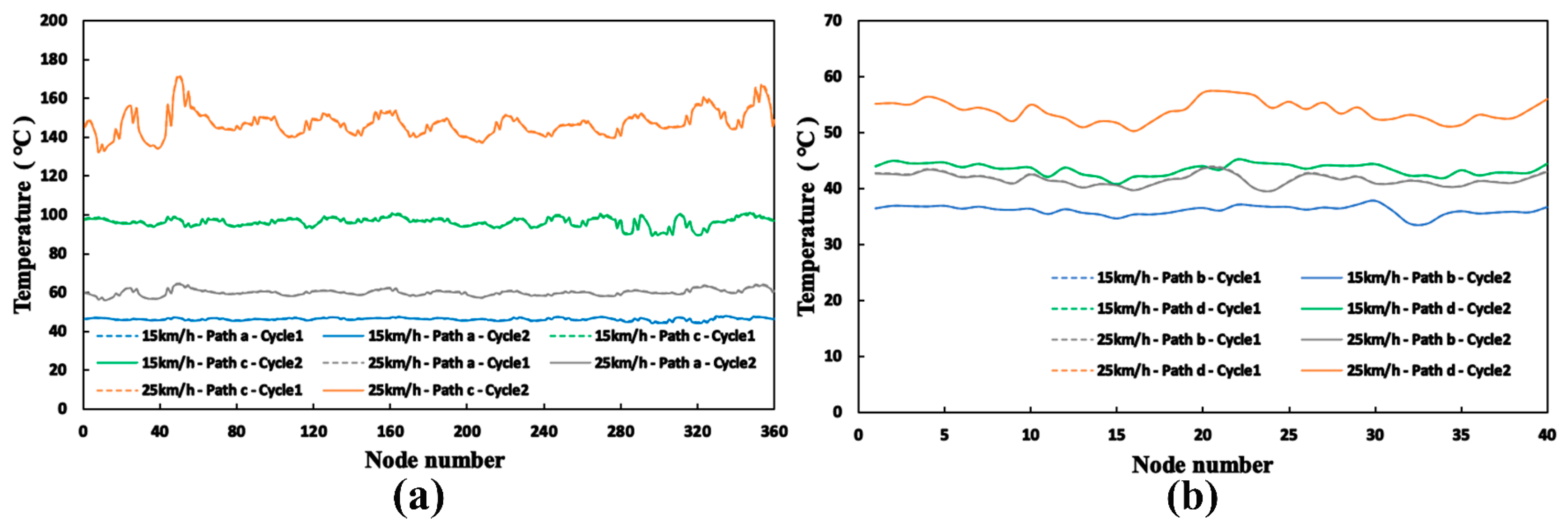
3.6. Steady-State Temperature Field and Rolling Resistance of the LSL-Tire under Different Speeds

The SSTF of the LSL-tire was simulated, and the rolling resistance was solved at the 15 km/h and 25 km/h velocities under the 520 N load. The temperature field under each condition also attained a steady state after two iterations. The iterative curves pertaining to the temperature of the nodes in the four paths is illustrated in Figure 19. It can be observed that the steady-state temperature of each part of the LSL-tire increased with the increase in velocity, because higher velocity meant smaller T which caused larger $q_m$. Figure 19a indicates that the temperature difference between the outer surface center of the tread and the center of the tread increased significantly with the velocity, and that the average steady-state temperature increased by 108% and 145% under the two conditions, respectively. It can be observed from Figure 19b that the temperature difference between the outer surface center of the spokes and the center of the spokes increased with the velocity, and that the average steady-state temperature increased by 20% and 29.5%, respectively, under the two conditions. Figure 17c,d and Figure 20 indicate that the highest steady-state temperature points of the tread were located in the center of the tread and were 103.3 °C and 171.1 °C, respectively. Furthermore, the highest steady-state temperature points of spokes were located in the center of the joint between the spokes and the outer ring, which were 54.4 °C and 73.6 °C, respectively.

The RR contribution of each part of the LSL-tire under the two conditions is depicted in Figure 21. It can be observed that the RR increased with the velocity. This observation is occasioned by a complex balance of different trends; however, it is not apparent. First, the lag angle of viscoelastic materials decreased with frequency in the range of frequencies characteristic of the large-scale rolling tire deformations [1]. This effect tended to decrease the RR as speed increased. Second, the SSTF increased with speed, and the loss factor decreased with increasing temperature, which also tended to lower RR with increasing speed. These two effects, however, were more than offset by the increase in larger stress and strain amplitudes occasioned by the tire deformation that occurred with increasing speed due to centrifugal forces. Reference [20] also describes that the rolling angular velocity exerts no significant effect on the RR of the honeycomb structure NPTs. The RR of the LSL-tire under the two conditions was 74.3 N and 75.2 N, respectively, and the growth rate was 1.2%. The spokes exerted the most considerable influence on the RR, accounting for 63.1% and 62.9% under the two conditions, followed by the tread, accounting for 28.9% and 29.1%, respectively.

4. Conclusions

An SSTF–RR solution strategy, based on explicit transient rolling analysis and thermal–mechanical coupling is proposed, being suitable for tires with complex patterns and NPTs. Based on the method, the SSTF and RR of the LSL-tire under different loads and velocities were analyzed, and the following conclusions were obtained:

(1)

Based on the SSTF experimental data of the LSL-tire, the accuracy of the solution strategy is verified, whose prediction accuracy pertaining to the SSTF of the tread outer surface center and the spoke outer surface center are 92.44% and 93.06%, respectively.

(2)

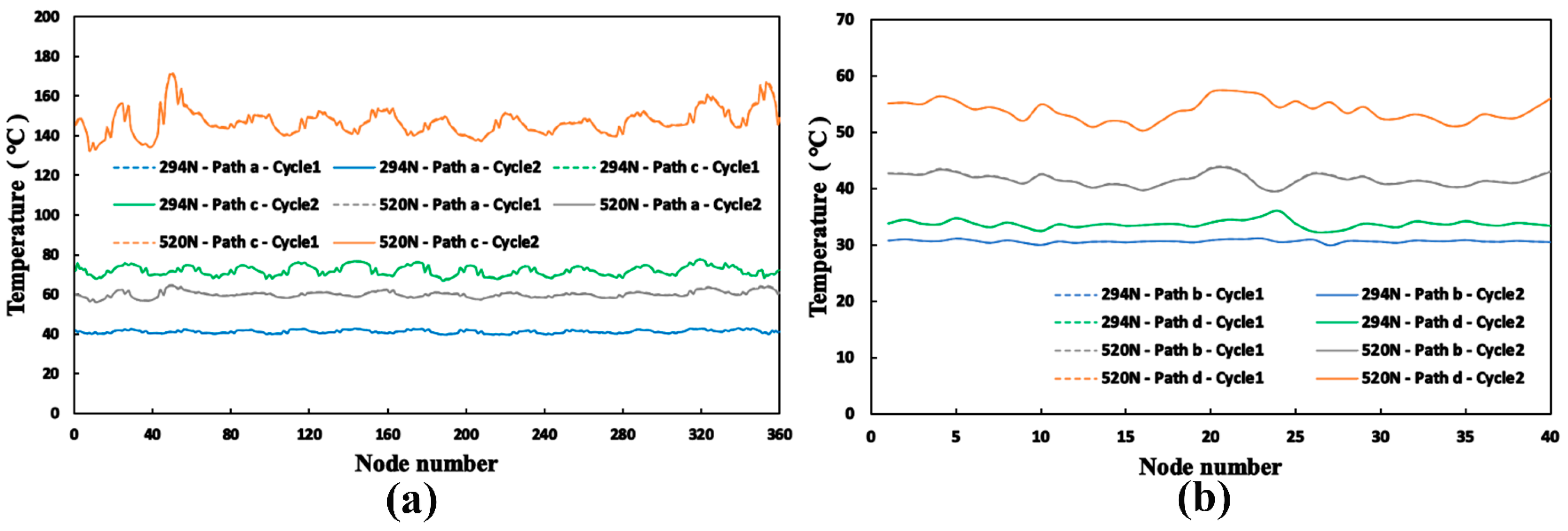
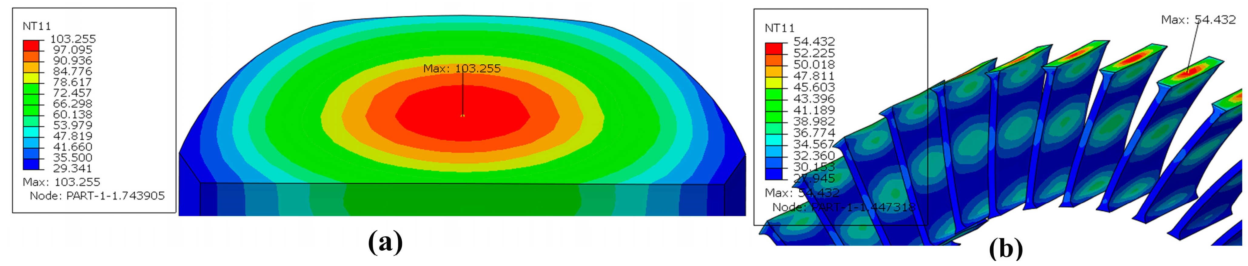
The SSTF of each part of the LSL-tire increases significantly with increases in load and velocity. The highest temperature point of the LSL-tire is located in the center of the tread, and the highest temperature point of the spokes is located in the center of the joint between spokes and the outer ring.

(3)

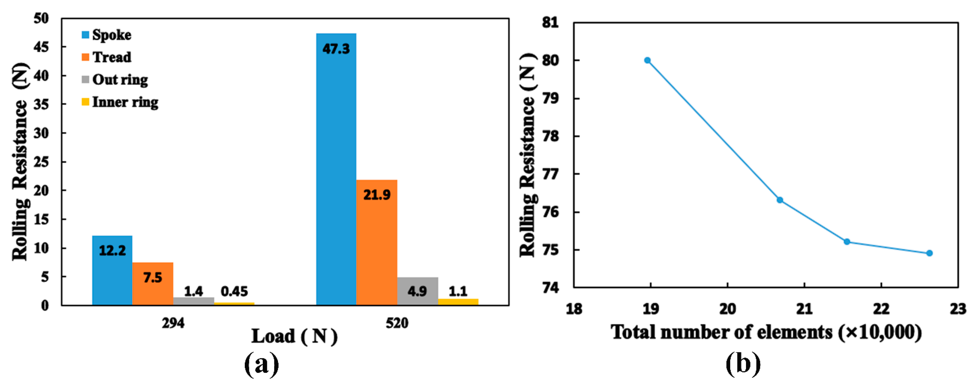
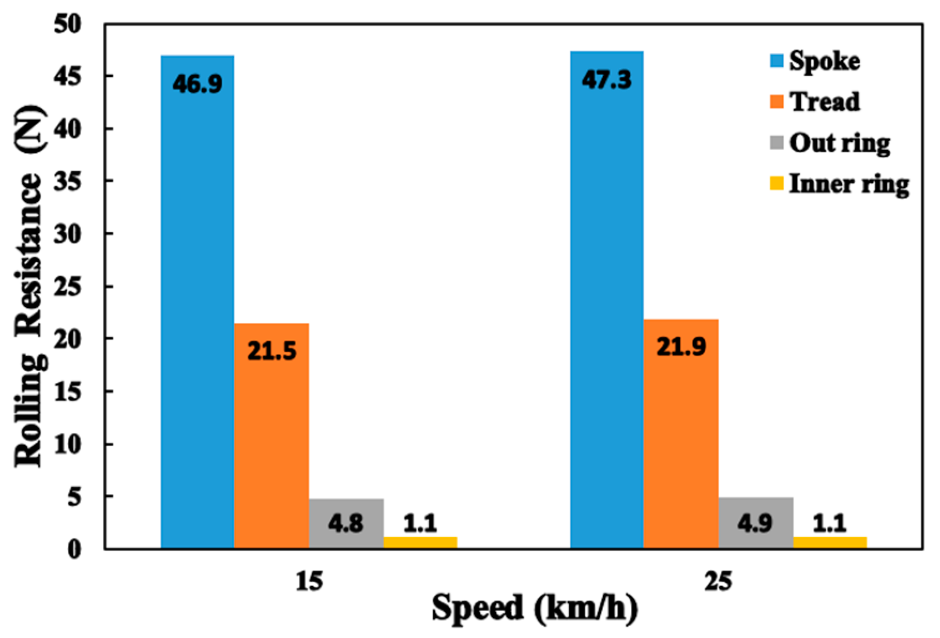
The RR of the LSL-tire increases significantly with increases in load, and the spokes exert the most considerable effect on the RR, followed by the tread.

(4)

The RR of the LSL-tire increases marginally with velocity.

(5)

The SSTF solution strategy proposed herein differs from the existing SSTF research methods; the strategy does not assume that the steady-state temperature of each radial cross-section of the tire is the same.

(6)

The SSTF and hysteresis energy loss solution strategy proposed herein can theoretically be applied to any object composed of viscoelastic materials, not only to tires.

References

1. Hall, D.E.; Moreland, J.C. Fundamentals of Rolling Resistance. Rubber Chem. Technol. 2001, 74, 525–539. [Google Scholar]
2. Xiong, Y. In-Plane Tire Deformation Measurement Using a Multi-Laser Sensor System. Ph.D. Thesis, Aalto University, Espoo, Finland, 2016. [Google Scholar]
3. Shida, Z.; Koishi, M.; Kogure, T.; Kabe, K. A Rolling Resistance Simulation of Tires Using Static Finite Element Analysis. Tire Sci. Technol. 1999, 27, 84–105. [Google Scholar] [CrossRef]
4. Koishi, M. Analysis of Rubber-Based Composite Materials Using Homogenization Method. Ph.D. Thesis, Yokohama National University, Yokohama, Japan, 1998. [Google Scholar]
5. Lin, Y.J.; Hwang, S.J. Temperature prediction of rolling tires by computer simulation. Math. Comput. Simul. 2004, 67, 235–246. [Google Scholar]
6. Tang, T.; Johnson, D.; Smith, R.E.; Felicelli, S.D. Numerical evaluation of the temperature field of steady-state rolling tires. Appl. Math. Model. 2013, 38, 1622–1637. [Google Scholar] [CrossRef]
7. Li, F.Z.; Liu, F.; Liu, J.; Gao, Y.Y.; Lu, Y.L.; Chen, J.F.; Yang, H.B.; Zhang, L.Q. Thermo-mechanical coupling analysis of transient temperature and rolling resistance for solid rubber tire: Numerical simulation and experimental verification. Compos. Sci. Technol. 2018, 167, 404–410. [Google Scholar]
8. Ulmer, J.D. Strain dependence of dynamic mechanical properties of carbon black-filled rubber compounds. Rubber Chem. Technol. 1996, 69, 15–47. [Google Scholar] [CrossRef]
9. Saux, V.L.; Marco, Y.; Calloch, S.; Charrier, P.; Taveau, D. Heat build-up of rubber under cyclic loadings: Validation of an efficient demarch to predict the temperature fields. Rubber Chem. Technol. 2013, 86, 38–56. [Google Scholar] [CrossRef]
10. Browne, A.L.; Wickliffe, L.E. Parametric study of convective heat transfer coefficients at the tire surface. Tire Sci. Technol. 1980, 8, 37–67. [Google Scholar] [CrossRef]
11. He, H.; Liu, J.M.; Zhang, Y.R.; Han, X.; Mars, W.V.; Zhang, L.Q.; Li, F.Z. Heat Build-Up and Rolling Resistance Analysis of a Solid Tire: Experimental Observation and Numerical Simulation with Thermo-Mechanical Coupling Method. Polymers 2022, 14, 2210–2230. [Google Scholar]
12. Ding, Y.M.; Wang, H.; ASCE, M.; Qian, J.Y.; Zhou, H.C. Evaluation of Tire Rolling Resistance from Tire-Deformable Pavement Interaction Modeling. J. Transp. Eng. Part B Pavements 2021, 147, 04021041. [Google Scholar]
13. Park, J.W.; Jeong, H.Y. Finite element modeling for the cap ply and rolling resistance of tires. Int. J. Automot. Technol. 2022, 23, 1427–1436. [Google Scholar] [CrossRef]
14. Cho, J.R.; Lee, H.W.; Jeong, W.B.; Jeong, K.M.; Kim, K.W. Numerical estimation of rolling resistance and temperature distribution of 3-D periodic patterned tire. Int. J. Solids Struct. 2013, 50, 86–96. [Google Scholar] [CrossRef]
15. Cho, J.R.; Lee, H.W.; Jeong, W.B.; Jeong, K.M.; Kim, K.W. Finite element estimation of hysteretic loss and rolling resistance of 3-D patterned tire. Int. J. Mech. Mater. Des. 2013, 9, 355–366. [Google Scholar] [CrossRef]
16. Lee, H.W.; Cho, J.R.; Jeong, W.B.; Jeong, K.M.; Kim, K.W. Mesh generation and hysteretic loss prediction of 3-D periodic patterned tire. Int. J. Automot. Technol. 2014, 15, 411–417. [Google Scholar] [CrossRef]
17. Fu, H.X.; Liang, X.M.; Wang, Y.; Ku, L.Y.; Xiao, Z. Thermal Mechanical Coupling Analysis of a Flexible Spoke Non-pneumatic Tire. J. Mech. Eng. 2022, 68, 143–154. [Google Scholar] [CrossRef]
18. Marin, M.; Chirila, A.; Öchsner, A.; Vlase, S. About finite energy solutions in thermoelasticity of micropolar bodies with voids. Bound. Value Probl. 2019, 2019, 89. [Google Scholar] [CrossRef]
19. Kim, K.; Heo, H.; Uddin, M.; Ju, J.; Kim, D.M. Optimization of Nonpneumatic Tire with Hexagonal Lattice Spokes for Reducing Rolling Resistance; SAE Technical Paper; SAE: Warrendale, PA, USA, 2015. [Google Scholar] [CrossRef]
20. Yoo, S.; Uddin, M.S.; Heo, H.; Ju, j.; Kim, D.M.; Choi, S.J. Deformation and Heat Generation in a Nonpneumatic Tire with Lattice Spokes; SAE Technical Paper; SAE: Warrendale, PA, USA, 2015. [Google Scholar] [CrossRef]
21. Yoo, S.; Uddin, M.S.; Heo, H.; Ju, j.; Choi, S.J. Thermoviscoelastic modeling of a nonpneumatic tire with a lattice spoke. Proc. Inst. Mech. Eng. Part D J. Automob. Eng. 2017, 231, 241–252. [Google Scholar] [CrossRef]
22. Jin, X.C.; Hou, C.; Fan, X.L.; Sun, Y.L.; Lv, J.N.; Lu, C.S. Investigation on the static and dynamic behaviors of non-pneumatic tires with honeycomb spokes. Compos. Struct. 2018, 187, 27–35. [Google Scholar] [CrossRef]
23. Veeramurthy, M. Modeling, Finite Element Analysis, and Optimization of Non-Pneumatic Tire (NPT) for the Minimization of Rolling Resistance. Master’s Thesis, Clemson University, Clemson, SC, USA, 2011. [Google Scholar]
24. Veeramurthy, M.; Ju, J.; Thompson, L.L.; Summers, J.D. Optimization of a non-pneumatic tire for reduced rolling resistance. In Proceedings of the IDETC/CIE, Washington, DC, USA, 28–31 August 2011. [Google Scholar]
25. Veeramurthy, M.; Ju, J.; Thompson, L.L.; Summers, J.D. Optimisation of geometry and material properties of a non-pneumatic tyre for reducing rolling resistance. Int. J. Veh. Des. 2014, 66, 193–216. [Google Scholar] [CrossRef]
26. Aldhufairi, H.S.; Essa, K.E. Tire rolling-resistance computation based on material viscoelasticity representation. Adv. Automot. Eng. 2019, 1, 167–183. [Google Scholar]
27. Aldhufairi, H.; Olatunbosun, R.; Essa, K. Determination of a Tyre’s Rolling Resistance Using Parallel Rheological Framework; SAE Technical Paper; SAE: Warrendale, PA, USA, 2019. [Google Scholar]
28. Kiran, M.; Aswath, M.; Shishir, D.A.; Ponangi, B.R.; Bhanumurthy, R. Effect of Material Models on Rolling Resistance of Non-pneumatic Tires with Hexagonal Spokes. SAE Int. J. Commer. Veh. 2023, 16, 33–47. [Google Scholar] [CrossRef]
29. GB/T 42825-2023; General Technical Specification of Electric Scooters. Standards Press of China: Beijing, China, 2023.
30. Garman, C.M.R.; Como, S.G.; Campbell, I.C.; Wishart, J.; O’Brien, K.; Lean, S.M. Micro-Mobility Vehicle Dynamics and Rider Kinematics during Electric Scooter Riding; SAE Technical Paper; SAE: Warrendale, PA, USA, 2020. [Google Scholar] [CrossRef]
31. T/ZZB 1970-2020; Electric Balancing Car Tires. Market Supervision Administration of Zhejiang Province: Hangzhou, China, 2020.
32. Nie, Y.Q.; Meng, G.W. Mechanics of Materials; China Machine Press: Beijing, China, 2009. [Google Scholar]
33. Wu, W.T. Simulation Analysis of Tire Temperature Field. Master’s Thesis, Jilin University, Changchun, China, 2017. [Google Scholar]
34. GB/T 1040.2-2022; Plastics-Determination of Tensile Properties-Part 2: Test Conditions for Moulding and Extrusion Plastics. Standards Press of China: Beijing, China, 2022.
35. GB/T 528-2009; Rubber, Vulcanized or Thermoplastic-Determination of Tensile Stress-Strain Properties. Standards Press of China: Beijing, China, 2009.
36. GB/T 40396-2021; Test Method for Glass Transition Temperature of Polymer Matrix Composites-Dynamic Mechanical Analysis (DMA). Standards Press of China: Beijing, China, 2021.
37. GB/T 19466.4-2016; Plastics-Differential Scanning Calorimetry (DSC)-Part 4: Determination of Specific Heat Capacity. Standards Press of China: Beijing, China, 2016.
38. GB/T 22588-2008; Determination of Thermal Diffusivity or Thermal Conductivity by the Flash Method. Standards Press of China: Beijing, China, 2008.
39. Liu, W.; Liu, S.; Li, X.; Zhang, Q.; Wang, C.; Li, K. Static Stiffness Properties of High Load Capacity Non-Pneumatic Tires with Different Tread Structures. Lubricants 2023, 11, 180. [Google Scholar]
Figure 1. Structural diagram of the LSL-tire: (a) geometric parameters of the LSL-tire; (b) profile of the LSL-tire.
Lubricants 11 00402 g001
Figure 2. Hysteresis effect of viscoelastic materials: (a) sinusoidal strain and stress; (b) lagged loop.
Lubricants 11 00402 g002
Figure 3. Fitting curve of equivalent stress.
Lubricants 11 00402 g003
Figure 4. SSTF and RR analysis flow chart.
Lubricants 11 00402 g004
Figure 5. SSTF experiment of the LSL-tire: (a) rolling heating process of the LSL-tire; (b) infrared temperature measurement.
Lubricants 11 00402 g005
Figure 6. Uniaxial tensile test of materials: (a) tensile test of PU; (b) tensile test of rubber.
Lubricants 11 00402 g006
Figure 7. Thermodynamic tests of materials: (a) DMA test process; (b) DSC test process.
Lubricants 11 00402 g007
Figure 8. FE and simulating model: (a) FE model of the LSL-tire; (b) simulating model of the LSL-tire.
Lubricants 11 00402 g008
Figure 9. Material constitutive fitting: (a) Marlow constitutive of rubber; (b) Marlow constitutive of PU.
Lubricants 11 00402 g009
Figure 10. Stress–strain curves.
Lubricants 11 00402 g010
Figure 11. DMA results: (a) DMA curves of rubber; (b) DMA curves of PU.
Lubricants 11 00402 g011
Figure 12. Specific heat capacity curves.
Lubricants 11 00402 g012
Figure 13. Circumferential path of nodes.
Lubricants 11 00402 g013
Figure 14. The test and simulation results of the steady-state temperature of path a and b: (a) path a; (b) path b.
Lubricants 11 00402 g014
Figure 15. The overall steady-state temperature field distribution of the LSL-tire: (a) simulated temperature field distribution; (b) tested temperature field distribution.
Lubricants 11 00402 g015
Figure 16. Temperature iteration of the path under different loads: (a) paths a and c; (b) paths b and d.
Lubricants 11 00402 g016
Figure 17. Temperature cloud diagram of tread and spokes under different loads: (a) tread temperature cloud diagram under 294 N; (b) spoke temperature cloud diagram under 294 N; (c) tread temperature cloud diagram under 520 N; (d) spoke temperature cloud diagram under 520 N.
Lubricants 11 00402 g017
Figure 18. Rolling resistance: (a) rolling resistance of the LSL-tire under different loads; (b) convergence to the total number of finite elements.
Lubricants 11 00402 g018
Figure 19. Temperature iteration of the path under different speeds: (a) paths a and c; (b) paths b and d.
Lubricants 11 00402 g019
Figure 20. Temperature cloud diagram of tread and spokes at the 15 km/h speed: (a) tread temperature cloud diagram under 15 km/h; (b) spoke temperature cloud diagram under 15 km/h.
Lubricants 11 00402 g020
Figure 21. Rolling resistance of the LSL-tire under different speeds.
Lubricants 11 00402 g021