Physics-Informed Neural Network (PINN) for Solving Frictional Contact Temperature and Inversely Evaluating Relevant Input Parameters

Abstract

Ensuring precise prediction, monitoring, and control of frictional contact temperature is imperative for the design and operation of advanced equipment. Currently, the measurement of frictional contact temperature remains a formidable challenge, while the accuracy of simulation results from conventional numerical methods remains uncertain. In this study, a PINN model that incorporates physical information, such as partial differential equation (PDE) and boundary conditions, into neural networks is proposed to solve forward and inverse problems of frictional contact temperature. Compared to the traditional numerical calculation method, the preprocessing of the PINN is more convenient. Another noteworthy characteristic of the PINN is that it can combine data to obtain a more accurate temperature field and solve inverse problems to identify some unknown parameters. The experimental results substantiate that the PINN effectively resolves the forward problems of frictional contact temperature when provided with known input conditions. Additionally, the PINN demonstrates its ability to accurately predict the friction temperature field with an unknown input parameter, which is achieved by incorporating a limited quantity of easily measurable actual temperature data. The PINN can also be employed for the inverse identification of unknown parameters. Finally, the PINN exhibits potential in solving inverse problems associated with frictional contact temperature, even when multiple input parameters are unknown.

1. Introduction

Friction is mostly dissipated as heat. The temperature rise generated by frictional heat plays a crucial role in determining the operating state of high-performance equipment [1]. Elevated frictional contact temperature has the potential to cause lubrication film breakdown, to diminish material functionality, or to intensify friction and wear between components, ultimately impacting the overall performance, lifespan, and reliability of the equipment [2,3,4]. Therefore, it is imperative to accurately evaluate the frictional contact temperature to guarantee the secure functioning of equipment.

Friction temperature can be either measured by experiments [5] or calculated by numerical simulations. For experimental methods, temperature in the vicinity of the contact surface can be captured by using infrared thermography or thermocouples, while directly measuring the temperature at the contact interfaces remains a challenge. There are various numerical methods available for temperature estimations, including the finite element method, finite volume method, and finite difference method [6,7,8,9,10]. These traditional numerical techniques have undergone significant development and have been proven to be successful in simulating friction temperature fields. However, an inherent challenge associated with these methods lies in the precise determination of the boundary conditions of the simulation domain, leading to disparities between the simulated and actual temperatures [11].

With the development of artificial intelligence (AI), deep learning methods have been successfully applied in industrial manufacturing [12,13], computer vision [14,15], and natural language processing [16,17]. In recent years, AI approaches have been studied in relation to thermal problems in engineering. Peng [18] developed a data-driven model for rapidly predicting steady-state convective temperature fields of complex geometries based on convolutional neural networks. Zhu [19] used data-driven deep learning models to study the thermal effects of batteries, which can forecast the temperature at certain times and predict the temperature fluctuation of batteries for a long period. Numerous data-driven deep learning methods have demonstrated impressive performance, but obtaining a large amount of reliable data is a time-consuming and laborious task. Additionally, these data-driven deep learning methods often exhibit limited generalization capabilities and lack of universality.

The physics-informed neural network (PINN) combines deep learning with physical models and has been applied in many fields such as fluid mechanics [20,21], solid mechanics [22,23], and heat transfer [24,25]. The PINN is gradually developing in the field of tribology [26,27,28,29,30,31]. The PINN utilizes the robust fitting capacity of neural networks to represent physical variables within the constraints of governing equations, boundary conditions, and initial conditions. Compared to data-driven deep learning models, the PINN can be trained even in the absence of sufficient data.

The PINN has several advantages over traditional numerical computation methods [32]. Firstly, it obviates the necessity for mesh generation, simplifying the preprocessing procedures and rendering them applicable to complex structures. Secondly, the PINN is relatively efficient in handling high-dimensional problems, avoiding the dimensionality catastrophe that plagues traditional numerical methods [33]. Finally, the PINN can combine known actual data to solve inverse problems, such as identifying material parameters and unknown boundary conditions [34,35,36,37,38]. Cai [39] used the PINN to obtain temperature and velocity distributions under unknown thermal boundary conditions, a task that is typically challenging for conventional numerical techniques. Go [40] proposed a model for simulating real-time temperature fields based on the PINN, which is capable of accurately estimating the temperature distribution and heat flux of a given heat source, even with limited temperature data. A PINN-based hybrid thermal model was developed by Liao [41], which utilizes partially observable data obtained by an infrared camera to predict the temperature distribution and estimate the unknown material and process parameters that are not directly observable. Zhang [42] divided the composite material into multiple subdomains and then used PINN to acquire the temperature distribution. Pang [43] proposed a PINN approach for assessing the heat generation rate of lithium-ion batteries, and the experimental findings demonstrated that the proposed PINN approach exhibits favorable performance in estimating the heat generation rate of batteries.

In order to obtain the friction temperature field, traditional numerical methods mainly consider the heat transfer process under specified boundary conditions, such as heat flux, temperature, and convection. However, determining the heat partitioning coefficient (HPC) and convective heat transfer coefficient (CHTC) directly presents a significant challenge. To overcome this challenge, the present study employs the PINN to simulate the friction heat transfer process. The PINN model is able to effectively capture unknown parameters, including the HPC and CHTC, in combination with available data. Therefore, the PINN can not only address the forward problem of frictional contact temperature but can also perform inverse evaluations of unknown input parameters.

2. Theory and Methods

2.1. Heat-Transfer Theory

The transient heat conduction differential equation can be expressed as

$$\frac{\partial }{\partial x}\left(k\frac{\partial T}{\partial x}\right)+\frac{\partial }{\partial y}\left(k\frac{\partial T}{\partial y}\right)+\frac{\partial }{\partial z}\left(k\frac{\partial T}{\partial z}\right)+\dot{q}=\rho c\frac{\partial T}{\partial t}$$

(1)

where T is the temperature as a function of time t and spatial coordinates x, y and z, k is the thermal conductivity, $\rho$ is the density, c is the specific heat capacity, and $\dot{q}$ is the energy generated per unit volume.

When the internal heat source is not considered and only the two-dimensional steady-state heat transfer phenomenon is analyzed, Equation (1) can be expressed as

$$\frac{\partial }{\partial x}\left(k\frac{\partial T}{\partial x}\right)+\frac{\partial }{\partial y}\left(k\frac{\partial T}{\partial y}\right)=0$$

(2)

The boundary conditions of heat transfer problems can be categorized into three types: the Dirichlet boundary condition, the Neumann boundary condition, and the Robin boundary condition.

The Dirichlet boundary condition enforces a specific temperature at the boundary and can be expressed as follows:

$$T_w=T$$

(3)

where $T_w$ is the temperature of the boundary.

The Neumann boundary condition imposes a heat flux on the boundary and can be expressed as follows:

$$k{\left.\frac{\partial T}{\partial \overrightarrow{n}}\right|}_w=q$$

(4)

where q is the heat flux imposed on the boundary.

The Robin boundary condition can be expressed as follows:

$${\left.-k\frac{\partial T}{\partial n}\right|}_w=h\left(T_w-T_0\right)+\epsilon \sigma \left(T_w^4-T_0^4\right)$$

(5)

where h is the CHTC at the surface, $T_w$ is the temperature of the boundary, $\epsilon$ is the radiant emissivity of the component, $\mathsf{\sigma }$ is the Stefan–Boltzmann constant with the value of 5.699 × 10⁻⁸ $\mathrm{W}/{\mathrm{m}}^2·{\mathrm{K}}^4$, and $T_0$ is the ambient temperature.

2.2. Frictional Contact-Temperature Simulation Method

Figure 1a illustrates the friction process between the two components. The total heat flux at the interface during the friction process is determined by the friction force and sliding speed. The total heat flux at the friction interface will be divided into two parts, in which one portion flows into the upper sample, and the remaining portion flows into the lower sample.

When the HPC is given, the friction heat transfer process can be simplified. As shown in Figure 1b, the simulation of frictional contact temperature can be simplified to the heat conduction process of the upper sample, which is influenced by the partial total heat flux and other boundary conditions. The heat flux entering the contact surface of the upper sample can be represented as follows:

$$q_{up}=\alpha q_{total}$$

(6)

where $q_{total}$ is the total heat flux at the friction interface, $q_{up}$ is the heat flux flowing into the upper sample, and $\alpha$ is the HPC.

When the heat flux and other boundary conditions are given, the temperature distribution resulting from friction can be determined by solving Equation (2).

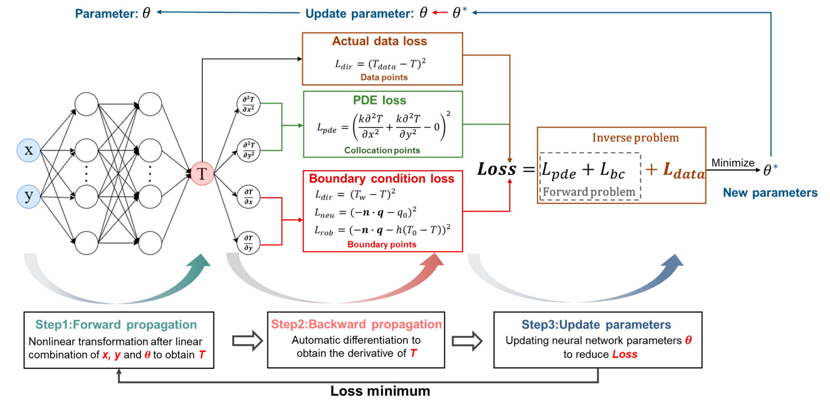
2.3. PINN Theory and Method

The PINN model incorporates essential physical information, such as partial differential equation (PDE) and boundary conditions, within a neural network framework. The exceptional fitting capability of neural networks allows them to effectively learn and approximate physical field variables, such as temperature. The automatic differentiation (AD) of neural networks allows for the direct derivation of differential terms in PDEs, eliminating the requirement for numerical techniques to compute the differentials. The PINN transforms the solution process for PDE with boundary conditions into a process that minimizes the residual of the PDE and boundary conditions. The neural network iteratively optimizes its parameters to ensure that the physical field variables satisfy both the constraints of the PDE and boundary conditions simultaneously.

Figure 2 shows the procedure of simulating frictional contact temperature by the PINN. In the initial step, as depicted in Figure 3, the collection points and actual data points are sampled within the computational domain. Subsequently, the neural network propagates forward to obtain the temperature of sampling points. For the second step, backpropagation is performed to calculate the partial differential of T with respect to x, y and $\theta$, respectively, and the loss for each part can be computed. Finally, the optimization algorithm is employed to update the parameters of the neural network, and the process is iterated until the residual of the loss reaches its minimum value [34,35].

When dealing with the forward problem of frictional contact temperature, the boundary conditions and material parameters of the computational domain are known, and the loss function can be expressed as follows:

$$L=L_{pde}+L_{bc}$$

(7)

where L is the total loss function, $L_{pde}$ is the loss function of PDE, and $L_{bc}$ is the loss function of the boundary condition.

When certain boundary conditions or material parameters within the computational domain are unknown, additional actual data need to be incorporated into the training of the PINN to guide the neural network’s training process and facilitate the determination of these unknown parameters. The temperature field predicted by the PINN must conform to both the PDE and boundary conditions, but also needs to satisfy the constraints of the actual data on the temperature field. The loss function can be expressed as follows:

$$L=L_{pde}+L_{bc}+L_{data}$$

(8)

where $L_{data}$ is the loss function of actual data.

During the optimization period, in addition to optimizing the parameters of the neural network, the unknown parameter p also needs to be updated. The parameter p can be unknown material parameters or the parameters representing boundary conditions, etc. The parameters that need to be optimized become $\theta \left(w,b,p\right)$, where w is the weight of the neural network, b is the bias of the neural network, and p is the unknown parameter that needs to be updated.

Many studies [44,45,46,47,48] have identified an optimization imbalance problem between different losses in PINN. This study employs the learning rate annealing method [49] to adapt the weights of each loss function, thereby facilitating comprehensive optimization of each individual loss. The total loss function can be expressed as

$$L=w_p{L}_{pde}+w_b{L}_{bc}+w_d{L}_{data}$$

(9)

where $w_p$, $w_b$ and $w_d$ are determined by the learning rate annealing method.

In this research, the training of the PINN is performed using GPU acceleration, specifically on an NVIDIA^® Tesla^® V100-SXM2, and relies predominantly on the PyTorch library. The detailed specifications of the GPU are provided as follows: GPU memory capacity: 32 GB, CUDA Cores: 5120, tensor cores: 640, single-precision floating-point performance: 15.7 TeraFLOPS, double-precision floating-point performance: 7.8 TeraFLOPS, FP16 tensor core performance: 125 TeraFLOPS. We employ a fully connected neural network with 9 hidden layers and 30 neurons per layer. The parameters of the neural network are randomly initialized by the Kaiming initialization method, the activation function used is swish, and the Adam optimizer is used for optimization. The initial learning rate is 2 × 10⁻⁴, and the value of the learning rate is automatically reduced when the loss no longer decreases within 100 iteration steps. To ensure complete convergence of the PINN, each neural network underwent training for 30,000 iterations, with a training time of approximately 1 h on our computer. The initial weights of each loss function were w_p = 0.1, w_b = 0.12, and w_d = 0.4, respectively, and the loss function weights were updated every 300 iterations during this process.

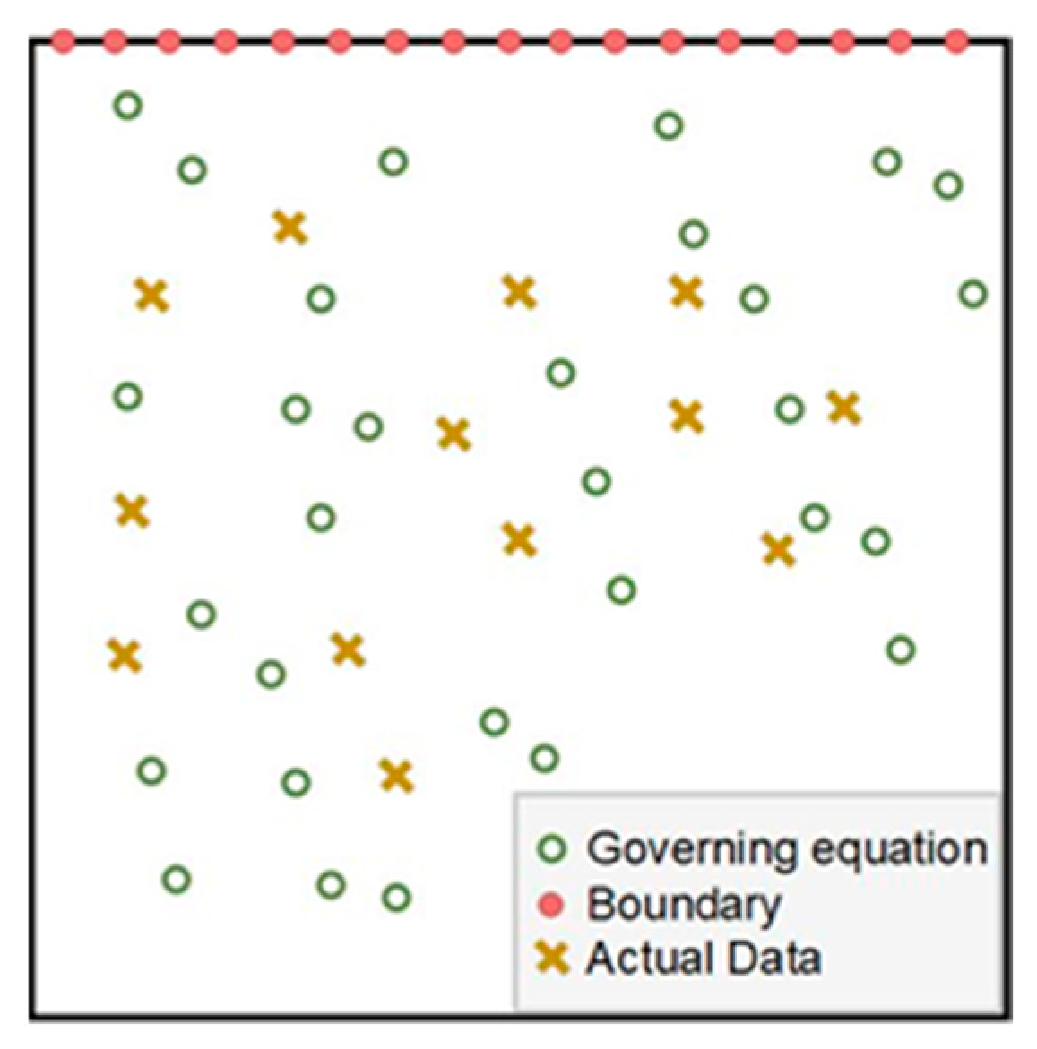
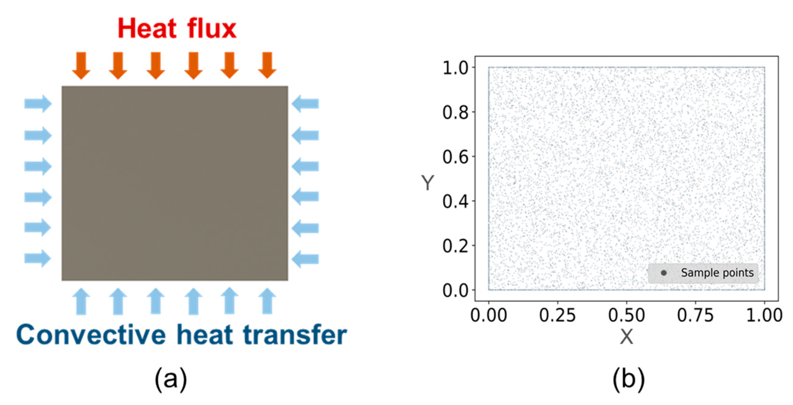
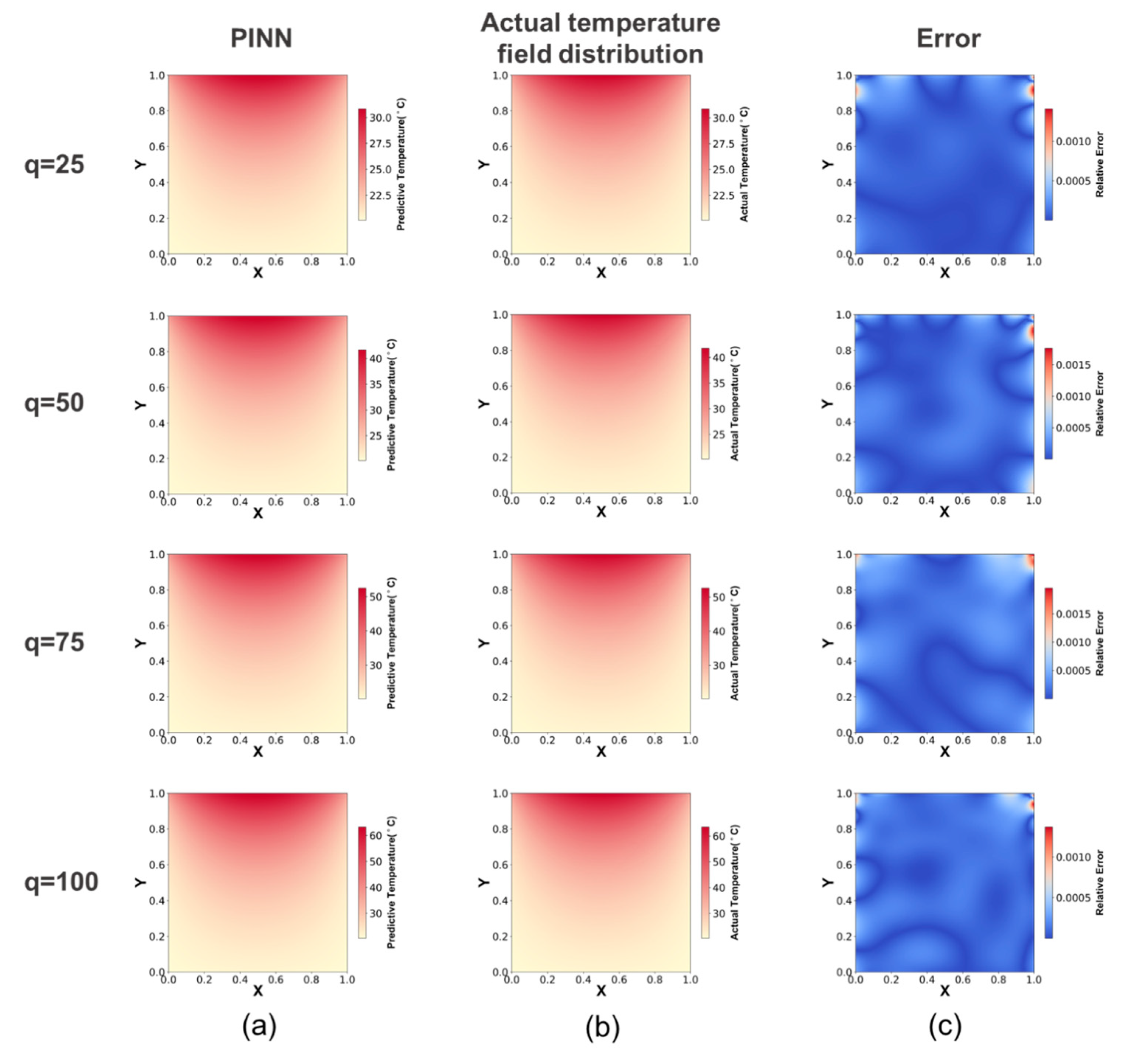
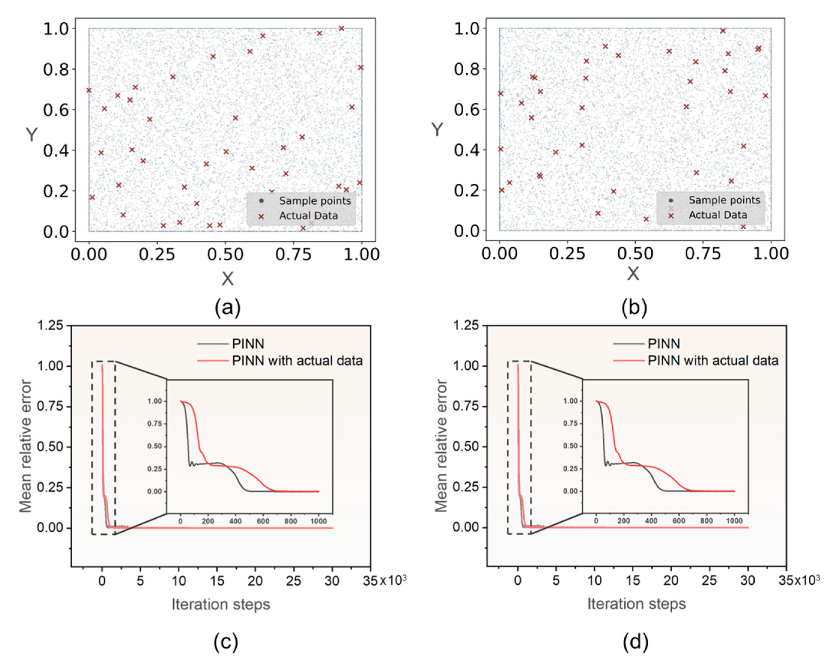
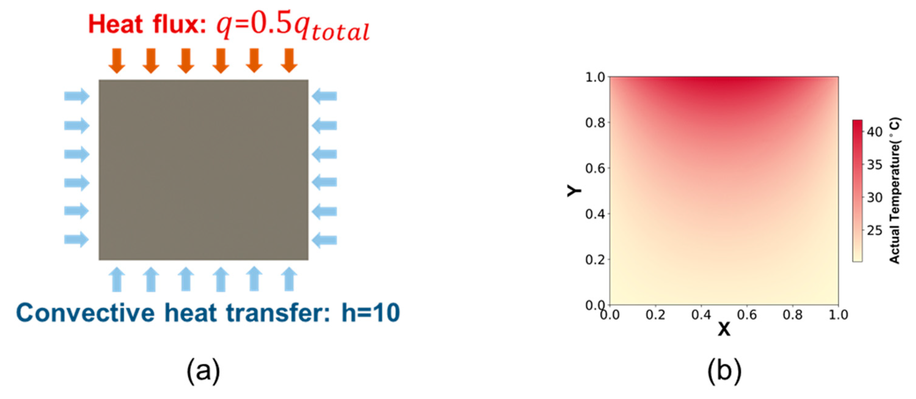
3. Frictional Contact Temperature Forward Calculation by the PINN

The forward calculation of frictional contact temperature by the PINN, as shown in Figure 4a, primarily involves the calculation of heat transfer within the sample subjected to known Neumann and Robin boundary conditions. The spatial distribution of collection points is visualized in Figure 4b, illustrating the random selection of 10,000 points within the computational domain, with an additional 500 points collected at each boundary. It is imperative that the temperature of all collection points within the computational domain needs to satisfy the PDE, while the temperature of the boundary collection points must satisfy the specified boundary conditions.

The basic parameters of the simulation are presented in

Table 1. Basic parameters for frictional contact temperature forward calculation.

Heat Flux $\mathbf{W}/{\mathbf{m}}^2$	CHTC $\mathbf{W}/\left({\mathbf{m}}^2·\mathbf{K}\right)$	Ambient Temperature °C	X, Y Length m	Thermal Conductivity $\mathbf{W}/\left(\mathbf{m}·\mathbf{K}\right)$
(25, 50, 75, 100)	10	20	1	1

. This study performs four distinct sets of experiments, each involving different heat flux conditions, with the aim of simulating frictional contact temperature across a range of operational scenarios. The simulation results obtained by the PINN were compared with the actual temperature field distribution simulated by Comsol. The simulation accuracy of the PINN was quantified by the mean relative error (MRE). Figure 5a,b represent the simulation results obtained by the PINN and Comsol, respectively, and Figure 5c represents the relative error distribution of the PINN. Based on the experimental results, it is evident that the PINN is capable of accurately simulating frictional contact temperature. The MRE for various operational conditions is presented in

Table 2. MRE of the PINN and the PINN with actual data under different experimental conditions.

Heat Flux W/m2	PINN	PINN with Actual Data
25	0.008%	0.006%
50	0.013%	0.009%
75	0.019%	0.008%
100	0.012%	0.007%

.

The PINN can not only perform forward calculation under the constraints of PDE and boundary conditions, but can also be combined with actual data to assist the training process. Figure 6a,b illustrate the random selection of 40 actual data points within the computational domain, which were subsequently incorporated into the training process of the PINN. The MRE of the temperature field under various experimental conditions is presented in Table 2. Figure 6c,d depict the convergence curve of the PINN and PINN with actual data. According to the experimental results, it can be observed that the convergence rate of the PINN is relatively slower when actual data are incorporated into its training process compared to the convergence rate of the PINN without actual data. However, Table 2 reveals that the incorporation of actual data into the training process of the PINN enhances its predictive accuracy.

The slower convergence rate of the PINN with actual data may be attributed to a multitude of factors. After incorporating actual data, the optimization problem of the PINN becomes more complex. As the complexity of the model increases, the optimization process becomes challenging during the initial phase. Furthermore, the actual data will constrain the optimization direction of the PINN so that the model does not optimize along the fastest direction that satisfies the PDE and boundary conditions during the optimization process. However, when actual data are incorporated, the model can be further optimized in a favorable direction.

4. Frictional Contact Temperature Inverse Calculation by the PINN

Traditional numerical methods are frequently employed to solve forward problems in which the input parameters are well defined, and the physical field variables can be obtained by physical equations. According to the aforementioned findings, while the PINN has the capability to tackle the forward problem, its training process is time consuming and it is not as well developed as traditional numerical methods. Therefore, the PINN does not exhibit significant advantages compared to traditional numerical methods for solving forward problems.

In general, simulation results may not precisely mirror real-world scenarios due to disparities between the input conditions employed in simulations and the conditions that exist in reality. One notable benefit of the PINN, in comparison to traditional numerical methods, is its ability to effectively incorporate available actual data to address problems with ambiguous input conditions.

When the HPC and CHTC are given, the calculation of the frictional contact temperature can be simplified to the heat transfer process depicted in Figure 4a. In this section, the PINN, combined with actual data, is utilized to solve the frictional contact temperature under the ambiguous boundary conditions, and the HPC and CHTC can be obtained inversely. The actual temperature is obtained by Comsol under the experimental conditions shown in

Table 3. Actual experimental conditions.

Total Heat Flux W/m2	HPC (Top)	CHTC $\mathbf{W}/\left({\mathbf{m}}^2·\mathbf{K}\right)$ (Left, Right, Bottom)	Ambient Temperature °C	X, Y Length m	Thermal Conductivity $\mathbf{W}/\left(\mathbf{m}·\mathbf{K}\right)$
100	0.5	10	20	1	1

. The top boundary is the heat flux boundary condition, where the total heat flux is 100 W/m² and the HPC is 0.5; the boundary conditions on the left, right, and bottom are convective boundary conditions, with CHTC of 10 $\mathrm{W}/\left({\mathrm{m}}^2·\mathrm{K}\right)$ and ambient temperature of 20 °C. The experimental conditions and temperature distribution of the actual temperature field are shown in Figure 7b.

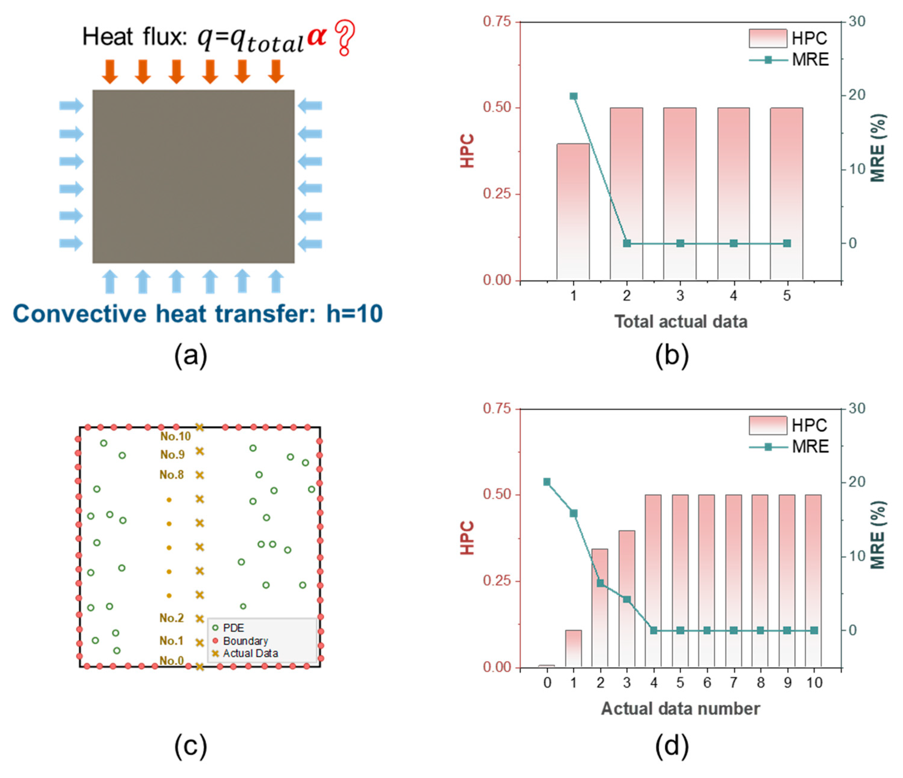
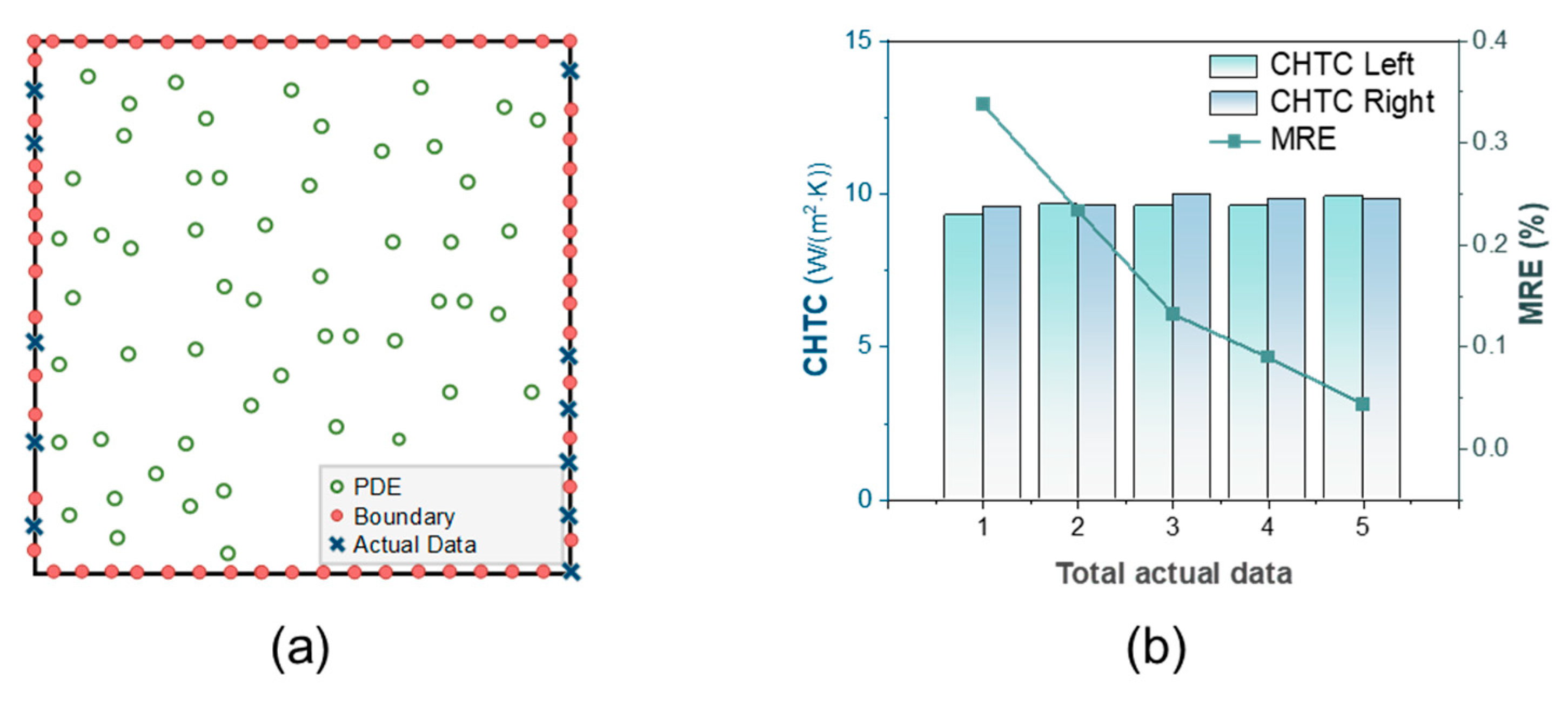
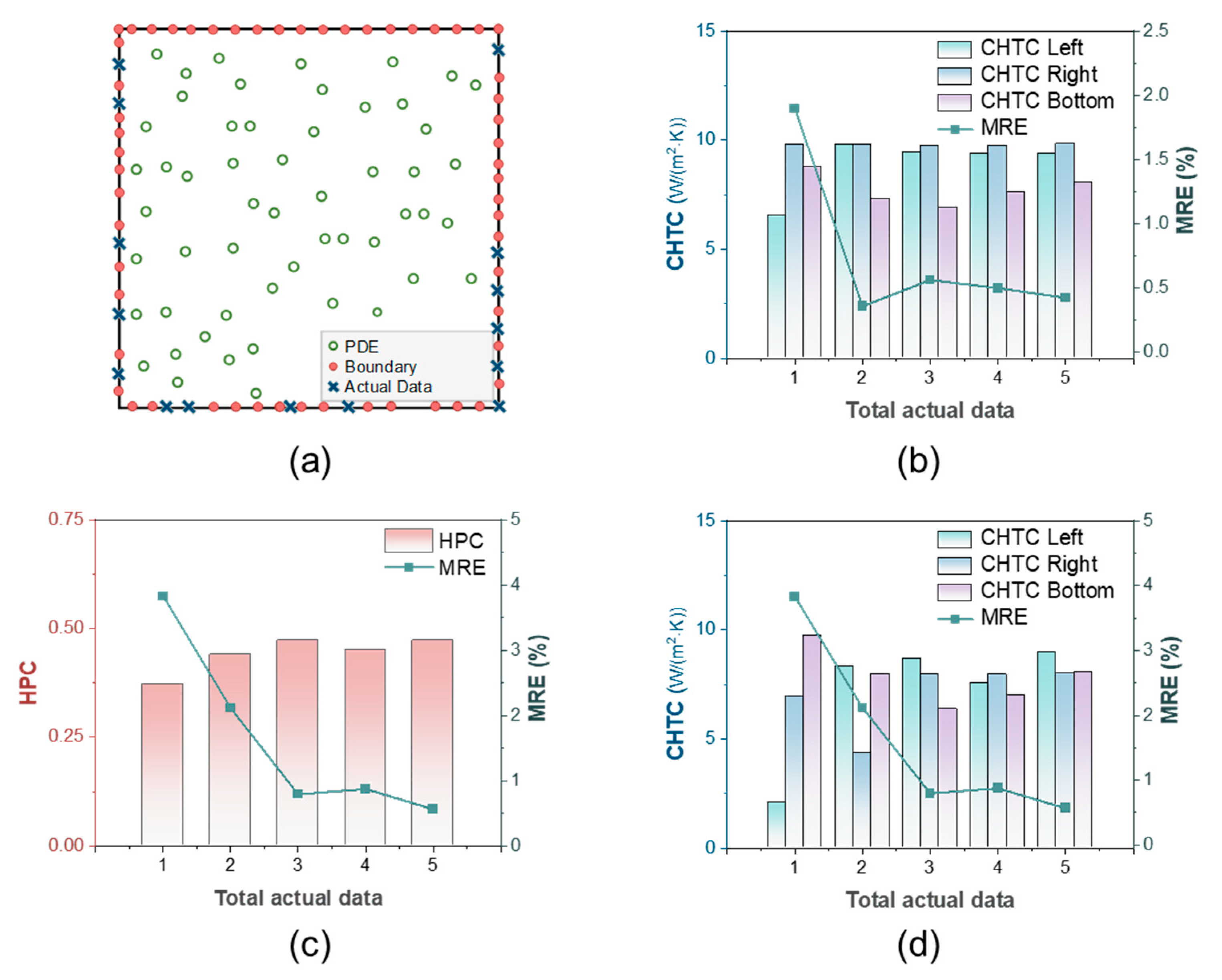
4.1. Inverse Problem for HPC

The total heat flux at the friction interface can be determined quite accurately based on the operating conditions; however, obtaining the HPC between the friction pairs under different working conditions poses a challenge [50]. Measuring the temperature at the interface of friction is a challenging task, while acquiring the temperature of the non-contact surface proves to be a comparatively straightforward task. The PINN can integrate the aforementioned available information. Specifically, it utilizes measurable known data to estimate the friction temperature distribution, even when the HPC is uncertain.

Figure 8a illustrates the boundary conditions of the simulation, where the HPC is the unknown input parameter to be optimized, with an initial value of 0.3. Initially, 1–5 actual data points are randomly collected within the computational domain and incorporated into the PINN to guide its training process. After completing the training process, the temperature distribution predicted by the PINN can be obtained, and the HPC can be inversely determined. Figure 8b shows the MRE of the PINN and the HPC as various datasets of actual data are incorporated into the training process. Accurate predictions of the friction temperature field and HPC can be achieved by incorporating only two actual data points into the training process. In addition, we also investigate the impact of actual data positions on the precision of the PINN. As depicted in Figure 8c, we collected the actual data from various positions, with the actual data from No.0 to No.10 gradually approaching the heat flux boundary, then incorporated each of these actual data into the training of the PINN. The predicted results of the PINN for actual data at different positions are shown in Figure 8d. It can be found that the position of actual data has a substantial impact on the prediction results of the PINN. As the actual data approaches the heat flux boundary, the errors of temperature field and HPC decrease from No.1 to No.4. The errors from No.4 to No.10 exhibit a tendency to remain consistent, and the HPC closely approximates the actual value. As the actual data approach the heat flux boundary, the temperature becomes increasingly influenced by the boundary. Consequently, the parameters of boundary conditions can be more accurately identified by utilizing actual data that are closer to the boundary. In Figure 8b, when actual data are incorporated into the training, the main reason for the relatively large error of MRE and HPC predicted by the PINN is that these actual data are located far away from the heat flux boundary.

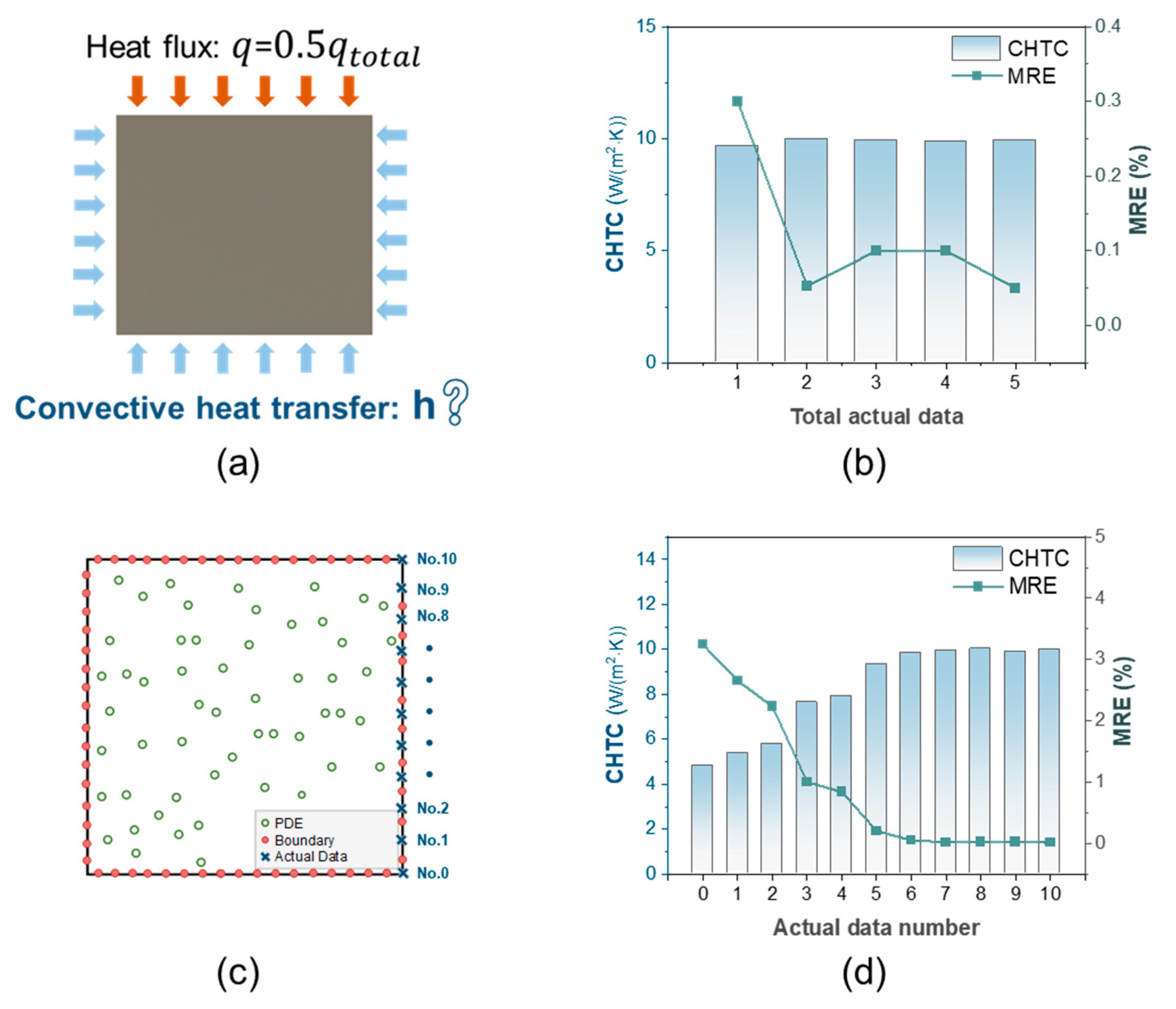
4.2. Inverse Problem for CHTC

Directly measuring the CHTC is challenging, often relying on empirical formulas [51]. An alternative approach involves employing computational fluid dynamics to simulate the fluid–solid coupling heat transfer process [52,53], however, this method is associated with significant costs. The surface temperature of an object is a readily measurable parameter. By incorporating these actual temperature data into the training of the PINN, the CHTC can be determined inversely.

Figure 9a illustrates the boundary conditions of the simulation, where the CHTC on the right boundary is the unknown input parameter to be optimized, with an initial value of 6$\mathrm{W}/\left({\mathrm{m}}^2·\mathrm{K}\right)$. Figure 9b shows the MRE of the PINN and the CHTC as various sets of actual data are incorporated into the training process. When only a single actual datum is incorporated into the training process, the PINN shows a relatively high MRE, but it exhibits superior performance in predicting CHTC. Furthermore, we also investigate the effect of actual data sampled from diverse positions at the boundary on the accuracy of the PINN. Figure 9c displays the positions of actual data at the convective boundary, and

Table 4. Actual temperature of each actual datum.

Actual Data Number	No.0	No.1	No.2	No.3	No.4	No.5	No.6	No.7	No.8	No.9	No.10
Temperature (°C)	20.2	20.4	20.6	20.8	21.2	21.6	22.1	22.8	23.8	25.3	28.2

presents the actual temperature for each actual data. The predicted results of the PINN for actual data at different sampling points are shown in Figure 9d, it can be found that the position of actual data significantly affects the accuracy of the PINN. From No.6 to No.10, the MRE of the PINN approaches its minimum value and shows signs of stabilization. However, substantial errors were observed in the experiments up to No.5, and the predictions of CHTC also exhibited significant discrepancies from the actual values. It can be found from Table 4 that the temperature risesfrom No.1 to No.5 were very small and close to the ambient temperature. Boundary conditions have minimal influence on the temperature at these specific points. Consequently, incorporating these points solely into the training process makes it challenging to constrain the optimization process of the PINN, resulting in poor accuracy when identifying unknown parameters.

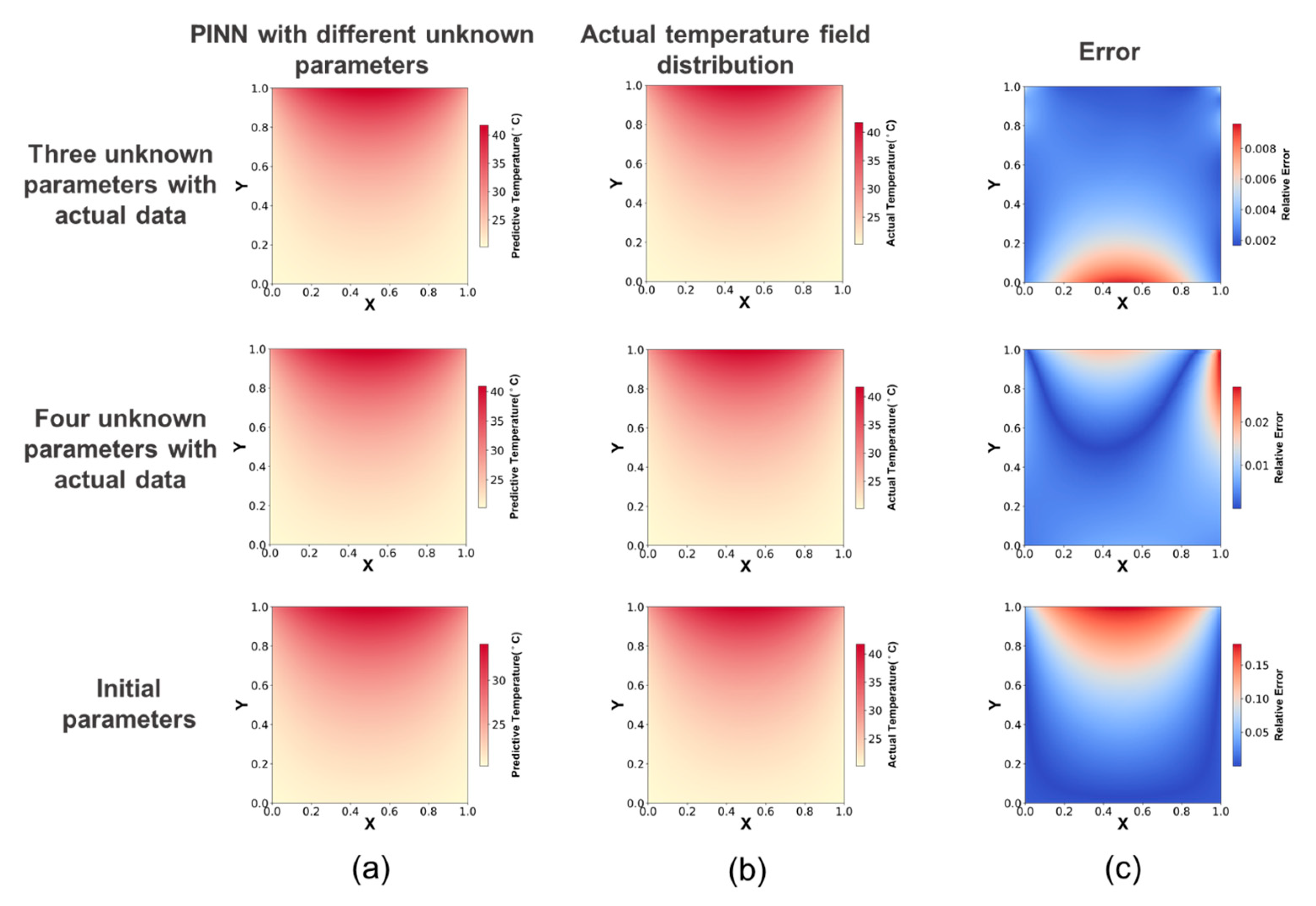
4.3. Inverse Problem for Multiple Unknown Parameters

Based on the aforementioned results, it is evident that the PINN has the capability to predict an unknown parameter by a limited amount of data. In real-world engineering scenarios, it is common for multiple parameters to remain unknown or undetermined. This section explores the application of the PINN when dealing with scenarios involving multiple unknown parameters.

The experimental conditions are shown in Table 3. In the case of two unknown CHTCs at the left and right boundaries, 1–5 actual data points are collected separately from the left and right boundaries, as depicted in Figure 10a. These data points are then incorporated into the training of the PINN. Figure 10b illustrates the MRE of the PINN and the two CHTCs as various datasets of actual data are integrated into the training process. The experimental findings demonstrate that by incorporating a limited quantity of actual data, the PINN can effectively predict the friction temperature field and provide more precise estimations for the actual values of two unknown CHTCs.

In cases in which all CHTCs are unknown, the actual data sampling is shown in Figure 11a. Figure 11b shows the MRE of the PINN and the three CHTCs as various datasets of actual data are incorporated into the training process. It is evident that the prediction error in the temperature field by the PINN, when dealing with three unknown parameters, is significant. The PINN exhibits greater accuracy in predicting the CHTCs at the left and right boundaries, while the prediction error for the CHTC at the bottom boundary is comparatively larger. Figure 11c,d illustrate the results of the PINN in cases in which all boundary input parameters are unknown. The temperature field predicted by the PINN shows significant errors, and the accuracy of predicting the unknown parameters at the four boundaries is also limited. Figure 12 and

Table 5. MRE of the PINN with different unknown parameters.

PINN with Different Unknown Parameters	Three Unknown Parameters with Actual Data	Four Unknown Parameters with Actual Data	Initial Parameters without Actual Data
MRE	0.03%	0.79%	5.16%

present the temperature field results and the MRE of the temperature field predicted by the PINN when all parameters are set to their initial values, indicating that they are unknown. It is observed from Figure 12 and Table 5 that incorporating a limited quantity of actual data into the PINN significantly reduces the prediction error of the temperature field, even in scenarios involving multiple unknown boundary parameters.

The PINN exhibits limited performance in solving inverse problems with multiple unknown parameters. As the number of unknown input parameters increases, the solution space expands into higher dimensions, resulting in a greater number of potential solutions. Training neural networks on high-dimensional problems presents challenges, as they are prone to trapping the neural network in local optima. On the other hand, the theoretical research on the PINN is still in its early stages. There are a large number of large hyperparameters in the PINN, and the prediction of many unknown parameters may require a better combination of hyperparameters. However, our experimental results demonstrate that the PINN effectively enhances the accuracy of temperature field prediction by incorporating a limited amount of actual data, which is still difficult for traditional numerical calculation methods.

5. Conclusions

In this study, a PINN model was introduced to solve both forward and inverse problems associated with frictional contact temperature. In situations in which the input boundary conditions are well defined, our study demonstrates that the PINN exhibits exceptional predictive accuracy cross various operational scenarios. Additionally, incorporating actual data into the training of the PINN may modestly decrease the convergence rate of forward problems while enhancing the prediction accuracy of the PINN. The maximum MRE decreased by approximately 0.01% in our experiment.

When an input thermal parameter, such as HPC or CHTC, is unknown, the PINN demonstrates the capability to accurately predict the frictional contact temperature field by incorporating just a single actual temperature data point during training, with an MRE of about 0.01–0.001%, and simultaneously, HPC and CHTC can be precisely identified by the optimization process of the PINN, with the relative error of about 0.01–0.1%. Experimental analysis revealed that the sampling positions of actual data play a significant role in influencing the predictive performance of the PINN. As the sampling points of actual data become closer to the boundary, the MRE of the temperature field decreases from 20.06% to 0.004% when the HPC is unknown, and from 3.25% to 0.01% when the HPCP is unknown. Incorporating actual data, which are strongly influenced by boundary conditions, into the training process can enhance the effectiveness of the PINN for solving inverse problems.

Finally, the study investigated the inverse thermal problem with multiple unknown input thermal parameters. The experimental results indicate that the PINN is successful at resolving cases involving two unknown CHTCs; the relative error of CHTCs is about 1–3%. In situations in which multiple input thermal parameters are unknown, the PINN exhibits relatively large errors in predicting the temperature field, and the HPC and CHTCs evaluated by the PINN deviate from the actual values. Nonetheless, incorporating a limited actual temperature data into the PINN can substantially enhance the accuracy of the frictional contact temperature field when all input thermal parameters are unknown. The MRE of the temperature field decreases from 5.16% to 0.79%.

The PINN demonstrates advantages in solving inverse thermal problems compared to traditional numerical methods, yet it is still in an early stage of development, and its theoretical basis and stability are not as robust as those of traditional forward numerical methods.

References

1. Meng, Y.; Xu, J.; Jin, Z.; Prakash, B.; Hu, Y. A Review of Recent Advances in Tribology. Friction 2020, 8, 221–300. [Google Scholar] [CrossRef]
2. Abdullah, O.I.; Schlattmann, J. Thermal Behavior of Friction Clutch Disc Based on Uniform Pressure and Uniform Wear Assumptions. Friction 2016, 4, 228–237. [Google Scholar] [CrossRef]
3. Lin, Z.; Qu, T.; Zhang, K.; Zhang, Q.; Wang, S.; Wang, G.; Gao, B.; Fan, G. Modeling of Contact Temperatures and Their Influence on the Tribological Performance of PEEK and PTFE in a Dual-Pin-on-Disk Tribometer. Friction 2023, 11, 546–566. [Google Scholar] [CrossRef]
4. Chang, L.; Zhang, G.; Wang, H.; Fu, K. Comparative Study on the Wear Behaviour of Two High-Temperature-Resistant Polymers. Tribol. Lett. 2017, 65, 34. [Google Scholar] [CrossRef]
5. Albers, A.; Klotz, T.; Fink, C.; Ott, S. Investigation of the Heat Distribution in Dry Friction Systems during Fade and Recovery Using Fiber-Optic Sensing and Infrared Technology. Friction 2022, 10, 422–435. [Google Scholar] [CrossRef]
6. Wang, H.; Liu, D.; Yan, L.; Wang, C.; Yang, S.; Zhu, Y. Tribological Simulation of Porous Self-Lubricating PEEK Composites with Heat-Stress Coupled Field. Tribol. Int. 2014, 77, 43–49. [Google Scholar] [CrossRef]
7. Ying, S.; Yupeng, Y. Temperature Field Analysis of Pin-on-Disk Sliding Friction Test. Int. J. Heat Mass Transf. 2017, 107, 339–346. [Google Scholar] [CrossRef]
8. Belhocine, A.; Bouchetara, M. Thermal Analysis of a Solid Brake Disc. Appl. Therm. Eng. 2012, 32, 59–67. [Google Scholar] [CrossRef]
9. Yevtushenko, A.A.; Adamowicz, A.; Grzes, P. Three-Dimensional FE Model for the Calculation of Temperature of a Disc Brake at Temperature-Dependent Coefficients of Friction. Int. Commun. Heat Mass Transf. 2013, 42, 18–24. [Google Scholar] [CrossRef]
10. Rahaman, M.L.; Zhang, L. Interface Temperature during Contact Sliding of Two Solids: Relationship between Predicted Flash Temperature and the Experimentally Measured. Proc. Inst. Mech. Eng. Part J J. Eng. Tribol. 2017, 231, 3–13. [Google Scholar] [CrossRef]
11. Xia, Y.; Yano, A.; Hayashi, N.; Horaguchi, N.; Xie, G.; Guo, D. Analysis of Temperature and Heat Partitioning Coefficient during Friction between Polymer and Steel. Tribol. Int. 2022, 171, 107561. [Google Scholar] [CrossRef]
12. Czimmermann, T.; Ciuti, G.; Milazzo, M.; Chiurazzi, M.; Roccella, S.; Oddo, C.M.; Dario, P. Visual-Based Defect Detection and Classification Approaches for Industrial Applications—A survey. Sensors 2020, 20, 1459. [Google Scholar] [CrossRef]
13. Chen, Y.; Ding, Y.; Zhao, F.; Zhang, E.; Wu, Z.; Shao, L. Surface Defect Detection Methods for Industrial Products: A Review. Appl. Sci. 2021, 11, 7657. [Google Scholar] [CrossRef]
14. Shah, A.; Shah, M.; Pandya, A.; Sushra, R.; Sushra, R.; Mehta, M.; Patel, K.; Patel, K. A Comprehensive Study on Skin Cancer Detection Using Artificial Neural Network (ANN) and Convolutional Neural Network (CNN). Clin. eHealth 2023, 6, 76–84. [Google Scholar] [CrossRef]
15. Mazurowski, M.A.; Dong, H.; Gu, H.; Yang, J.; Konz, N.; Zhang, Y. Segment Anything Model for Medical Image Analysis: An Experimental Study. Med. Image Anal. 2023, 89, 102918. [Google Scholar] [CrossRef]
16. Wang, X.; Zhang, X.; Cao, Y.; Wang, W.; Shen, C.; Huang, T. SegGPT: Towards Segmenting Everything in Context. In Proceedings of the IEEE/CVF International Conference on Computer Vision, Paris, France, 6 October 2023; pp. 1130–1140. [Google Scholar]
17. Zhao, W.X.; Zhou, K.; Li, J.; Tang, T.; Wang, X.; Hou, Y.; Min, Y.; Zhang, B.; Zhang, J.; Dong, Z.; et al. A Survey of Large Language Models. arXiv 2023, arXiv:2303.18223. [Google Scholar]
18. Peng, J.-Z.; Liu, X.; Aubry, N.; Chen, Z.; Wu, W.-T. Data-Driven Modeling of Geometry-Adaptive Steady Heat Conduction Based on Convolutional Neural Networks. Case Stud. Therm. Eng. 2021, 28, 101651. [Google Scholar] [CrossRef]
19. Zhu, S.; He, C.; Zhao, N.; Sha, J. Data-Driven Analysis on Thermal Effects and Temperature Changes of Lithium-Ion Battery. J. Power Sources 2021, 482, 228983. [Google Scholar] [CrossRef]
20. Raissi, M.; Yazdani, A.; Karniadakis, G.E. Hidden Fluid Mechanics: Learning Velocity and Pressure Fields from Flow Visualizations. Science 2020, 367, 1026–1030. [Google Scholar] [CrossRef] [PubMed]
21. Mao, Z.; Jagtap, A.D.; Karniadakis, G.E. Physics-Informed Neural Networks for High-Speed Flows. Comput. Methods Appl. Mech. Eng. 2020, 360, 112789. [Google Scholar] [CrossRef]
22. Zhang, E.; Dao, M.; Karniadakis, G.E.; Suresh, S. Analyses of Internal Structures and Defects in Materials Using Physics-Informed Neural Networks. Sci. Adv. 2022, 8, eabk0644. [Google Scholar] [CrossRef]
23. Haghighat, E.; Raissi, M.; Moure, A.; Gomez, H.; Juanes, R. A Physics-Informed Deep Learning Framework for Inversion and Surrogate Modeling in Solid Mechanics. Comput. Methods Appl. Mech. Eng. 2021, 379, 113741. [Google Scholar] [CrossRef]
24. Laubscher, R. Simulation of Multi-Species Flow and Heat Transfer Using Physics-Informed Neural Networks. Phys. Fluids 2021, 33, 087101. [Google Scholar] [CrossRef]
25. Xie, J.; Chai, Z.; Xu, L.; Ren, X.; Liu, S.; Chen, X. 3D Temperature Field Prediction in Direct Energy Deposition of Metals Using Physics Informed Neural Network. Int. J. Adv. Manuf. Technol. 2022, 119, 3449–3468. [Google Scholar] [CrossRef]
26. Fukushima, R.; Kano, M.; Hirahara, K. Physics-Informed Neural Networks for Fault Slip Monitoring: Simulation, Frictional Parameter Estimation, and Prediction on Slow Slip Events in a Spring-Slider System. J. Geophys. Res. Solid Earth 2023, 128, e2023JB027384. [Google Scholar] [CrossRef]
27. Marian, M.; Tremmel, S. Physics-Informed Machine Learning—An Emerging Trend in Tribology. Lubricants 2023, 11, 463. [Google Scholar] [CrossRef]
28. Olejnik, P.; Ayankoso, S. Friction Modelling and the Use of a Physics-Informed Neural Network for Estimating Frictional Torque Characteristics. Meccanica 2023, 58, 1885–1908. [Google Scholar] [CrossRef]
29. Zhao, Y.; Guo, L.; Wong, P.P.L. Application of Physics-Informed Neural Network in the Analysis of Hydrodynamic Lubrication. Friction 2023, 11, 1253–1264. [Google Scholar] [CrossRef]
30. Kurt, H.I.; Oduncuoglu, M. Application of a Neural Network Model for Prediction of Wear Properties of Ultrahigh Molecular Weight Polyethylene Composites. Int. J. Polym. Sci. 2015, 2015, e315710. [Google Scholar] [CrossRef]
31. Hasan, M.S.; Kordijazi, A.; Rohatgi, P.K.; Nosonovsky, M. Triboinformatic Modeling of Dry Friction and Wear of Aluminum Base Alloys Using Machine Learning Algorithms. Tribol. Int. 2021, 161, 107065. [Google Scholar] [CrossRef]
32. Markidis, S. The Old and the New: Can Physics-Informed Deep-Learning Replace Traditional Linear Solvers? Front. Big Data 2021, 4, 669097. [Google Scholar] [CrossRef]
33. Weinan, E.; Han, J.; Jentzen, A. Algorithms for Solving High Dimensional PDEs: From Nonlinear Monte Carlo to Machine Learning. Nonlinearity 2022, 35, 278–310. [Google Scholar] [CrossRef]
34. Yang, M.; Foster, J.T. Multi-Output Physics-Informed Neural Networks for Forward and Inverse PDE Problems with Uncertainties. Comput. Methods Appl. Mech. Eng. 2022, 402, 115041. [Google Scholar] [CrossRef]
35. Miao, Z.; Chen, Y. VC-PINN: Variable Coefficient Physics-Informed Neural Network for Forward and Inverse Problems of PDEs with Variable Coefficient. Phys. D Nonlinear Phenom. 2023, 456, 133945. [Google Scholar] [CrossRef]
36. Maddu, S.; Sturm, D.; Müller, C.L.; Sbalzarini, I.F. Inverse Dirichlet Weighting Enables Reliable Training of Physics Informed Neural Networks. Mach. Learn. Sci. Technol. 2022, 3, 015026. [Google Scholar] [CrossRef]
37. Zhang, Z.-Y.; Zhang, H.; Liu, Y.; Li, J.-Y.; Liu, C.-B. Generalized Conditional Symmetry Enhanced Physics-Informed Neural Network and Application to the Forward and Inverse Problems of Nonlinear Diffusion Equations. Chaos Solitons Fractals 2023, 168, 113169. [Google Scholar] [CrossRef]
38. Xu, C.; Cao, B.T.; Yuan, Y.; Meschke, G. Transfer Learning Based Physics-Informed Neural Networks for Solving Inverse Problems in Engineering Structures under Different Loading Scenarios. Comput. Methods Appl. Mech. Eng. 2023, 405, 115852. [Google Scholar] [CrossRef]
39. Cai, S.; Wang, Z.; Wang, S.; Perdikaris, P.; Karniadakis, G.E. Physics-Informed Neural Networks for Heat Transfer Problems. J. Heat Transf. 2021, 143, 060801. [Google Scholar] [CrossRef]
40. Go, M.-S.; Lim, J.H.; Lee, S. Physics-Informed Neural Network-Based Surrogate Model for a Virtual Thermal Sensor with Real-Time Simulation. Int. J. Heat Mass Transf. 2023, 214, 124392. [Google Scholar] [CrossRef]
41. Liao, S.; Xue, T.; Jeong, J.; Webster, S.; Ehmann, K.; Cao, J. Hybrid Thermal Modeling of Additive Manufacturing Processes Using Physics-Informed Neural Networks for Temperature Prediction and Parameter Identification. Comput. Mech. 2023, 72, 499–512. [Google Scholar] [CrossRef]
42. Zhang, B.; Wang, F.; Qiu, L. Multi-Domain Physics-Informed Neural Networks for Solving Transient Heat Conduction Problems in Multilayer Materials. J. Appl. Phys. 2023, 133, 245103. [Google Scholar] [CrossRef]
43. Pang, H.; Wu, L.; Liu, J.; Liu, X.; Liu, K. Physics-Informed Neural Network Approach for Heat Generation Rate Estimation of Lithium-Ion Battery under Various Driving Conditions. J. Energy Chem. 2023, 78, 1–12. [Google Scholar] [CrossRef]
44. McClenny, L.D.; Braga-Neto, U.M. Self-Adaptive Physics-Informed Neural Networks. J. Comput. Phys. 2023, 474, 111722. [Google Scholar] [CrossRef]
45. Shi, S.; Liu, D.; Null, R.J.; Han, Y. An Adaptive Physics-Informed Neural Network with Two-Stage Learning Strategy to Solve Partial Differential Equations. Numer. Math. Theor. Meth. Appl. 2023, 16, 298–322. [Google Scholar] [CrossRef]
46. Wang, S.; Yu, X.; Perdikaris, P. When and Why PINNs Fail to Train: A Neural Tangent Kernel Perspective. J. Comput. Phys. 2022, 449, 110768. [Google Scholar] [CrossRef]
47. Xiang, Z.; Peng, W.; Liu, X.; Yao, W. Self-Adaptive Loss Balanced Physics-Informed Neural Networks. Neurocomputing 2022, 496, 11–34. [Google Scholar] [CrossRef]
48. Cipolla, R.; Gal, Y.; Kendall, A. Multi-Task Learning Using Uncertainty to Weigh Losses for Scene Geometry and Semantics; IEEE: Piscataway, NJ, USA, 2018; ISBN 978-1-5386-6420-9. [Google Scholar]
49. Wang, S.; Teng, Y.; Perdikaris, P. Understanding and Mitigating Gradient Flow Pathologies in Physics-Informed Neural Networks. SIAM J. Sci. Comput. 2021, 43, A3055–A3081. [Google Scholar] [CrossRef]
50. Xiong, C.; Chen, M.; Yu, L. Analytical Model and Material Equivalent Methods for Steady State Heat Partition Coefficient between Two Contact Discs in Multi-Disc Clutch. Proc. Inst. Mech. Eng. Part D J. Automob. Eng. 2020, 234, 857–871. [Google Scholar] [CrossRef]
51. Longo, G.A.; Gasparella, A. Refrigerant R134a Vaporisation Heat Transfer and Pressure Drop inside a Small Brazed Plate Heat Exchanger. Int. J. Refrig. 2007, 30, 821–830. [Google Scholar] [CrossRef]
52. Vollaro, A.D.L.; Galli, G.; Vallati, A. CFD Analysis of Convective Heat Transfer Coefficient on External Surfaces of Buildings. Sustainability 2015, 7, 9088–9099. [Google Scholar] [CrossRef]
53. Kuwahara, F.; Shirota, M.; Nakayama, A. A Numerical Study of Interfacial Convective Heat Transfer Coefficient in Two-Energy Equation Model for Convection in Porous Media. Int. J. Heat Mass Transf. 2001, 44, 1153–1159. [Google Scholar] [CrossRef]
Figure 1. Friction heat transfer process. (a) Overall model of frictional heat transfer. (b) Simplified model for frictional heat transfer.
Lubricants 12 00062 g001
Figure 2. Simulation of frictional contact temperature based on the PINN.
Lubricants 12 00062 g002
Figure 3. Sampling of collection points and actual data points within the computational domain.
Lubricants 12 00062 g003
Figure 4. (a) Boundary conditions of forward calculation. (b) Sampling position of collection points.
Lubricants 12 00062 g004
Figure 5. Temperature field results and relative errors. (a) Simulation results of the PINN. (b) Actual temperature field distribution simulated by Comsol. (c) Relative error of the PINN.
Lubricants 12 00062 g005
Figure 6. Actual data sampling and MRE convergence process. (a,c) represent the sampling position of actual data points and MRE convergence process when the heat flux is 50 W/m2. (b,d) are the sampling position of actual data points and MRE convergence process when the heat flux is 100 W/m2.
Lubricants 12 00062 g006
Figure 7. Actual temperature field. (a) Experimental conditions. (b) Actual temperature field distribution.
Lubricants 12 00062 g007
Figure 8. Inverse problem for HPC. (a) Boundary conditions. (b) HPC and MRE of the PINN with different total actual data. (c) Actual data sampling at different positions. (d) HPC and MRE of the PINN with actual data from different positions.
Lubricants 12 00062 g008
Figure 9. Inverse problem for CHTC. (a) Boundary conditions. (b) CHTC and MRE of the PINN with different total actual data. (c) Actual data sampling at different positions. (d) CHTC and MRE of the PINN with actual data from different positions.
Lubricants 12 00062 g009
Figure 10. Sampling and results of two unknown parameters. (a) Actual data sampling of two unknown CHTCs. (b) Two CHTCs and MRE of the PINN with different total actual data.
Lubricants 12 00062 g010
Figure 11. Results of multiple unknown parameters. (a) Actual data sampling of three unknown CHTCs. (b) Three CHTCs and MRE of the PINN with different total actual data. (c) HPC and MRE of the PINN with four unknown parameters. (d) CHTCs and MRE of the PINN with four unknown parameters.
Lubricants 12 00062 g011
Figure 12. Temperature field predicted by the PINN. (a) Temperature field predicted by the PINN with different unknown parameters. (b) Actual temperature field distribution. (c) Relative error of the PINN.
Lubricants 12 00062 g012