Abstract
Understanding and predicting the friction between a steel runner and an ice surface is paramount for many winter sports disciplines such as luge, bobsleigh, skeleton, and speed skating. A widely used numerical model for the analysis of the tribological system steel-on-ice is the Friction Algorithm using Skate Thermohydrodynamics (F.A.S.T.), which was originally introduced in 2007 and later extended. It aims to predict the resulting coefficient of friction (COF) from the two contributions of ice plowing and viscous drag. We explore the limitations of the existing F.A.S.T. model and extend the model to improve its applicability to winter sports disciplines. This includes generalizing the geometry of the runner as well as the curvature of the ice surface. The free rotational mechanical mounting of the runner to the moving sports equipment is introduced and implemented. We apply the new model to real-world geometries and kinematics of speed skating blades and bobsleigh runners to determine the resulting COF for a range of parameters, including geometry, temperature, load, and speed. The findings are compared to rule-of-thumb testimonies from athletes, previous numerical approaches, and published experimental results where applicable. While the general trends are reproduced, some discrepancy is found, which we ascribe to the specific assumptions around the formation of the liquid water layer derived from melted ice.
1. Introduction
The interplay between ice and runners in winter sports presents a captivating nexus of physics, engineering, and athletic achievement. At the heart of competitive winter sports lies the relentless pursuit of performance optimization. Athletes and equipment manufacturers alike strive to gain a competitive edge. Understanding the complex dynamics governing frictional interactions is paramount for enhancing equipment design and, ultimately, achieving peak athletic performance.
Conducting experiments to study ice–steel friction in winter sports presents a unique set of challenges. The frictional forces involved are low, speeds are high, and results can vary significantly with respect to ice conditions, rendering experimental analysis costly and time-intensive.
Numerical simulations have emerged as indispensable tools in unraveling the intricacies of ice–runner friction. By leveraging computational models, researchers can explore a vast array of parameters and scenarios regarding the runners’ geometries, materials, climates, types of ice, kinematics, etc. Numerical simulations can thus offer unparalleled insights into the underlying physics of winter sports.
In this paper, we build on an existing popular model called Friction Algorithm using Skate Thermohydrodynamics (F.A.S.T.) to extend the scenarios to which it is applicable.
We start by introducing the previous generations of the F.A.S.T. model and laying out the basic principle of its numerical scheme. The main limitations and challenges resulting from this scheme are highlighted. We then introduce our additions to the model, extending its capabilities but also introducing new steps with significant computational costs. The accompanying challenges are discussed.
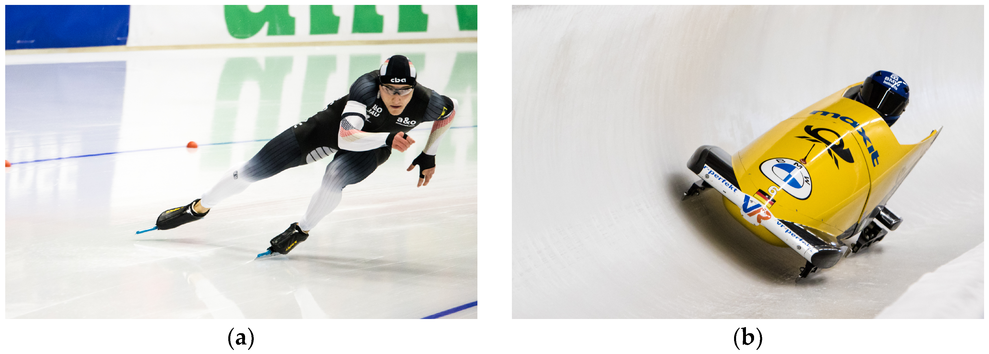
In Section 3, we then employ the new model to investigate cases of two major winter sports disciplines: speed skating and bobsleigh. Typical blade to ice configurations in these disciplines can be seen in Figure 1.

Figure 1.
Winter sports racing: (a) speed skater at the World Championships 2024 in Inzell and (b) bobsleigh pilot at the 2024 Monobob World Championship in Winterberg (©R. Hartnick).
2. Methods
In the following sections, the origin and fundamentals of the F.A.S.T. model are briefly summarized and the extensions made are presented.
2.1. F.A.S.T. Model
We start by looking at the history and current state of the F.A.S.T. model, as it was used as a starting point for our work.
2.1.1. Genesis of the F.A.S.T. Model
The F.A.S.T. model was originally developed in 2007 by Penny et al. for the sport of speed skating [1]. It was implemented for an upright speed skating blade and contained terms for plowing of the ice and shearing of the water layer, which is built through melting, heat conduction, and squeezing. In 2011, Lozowski and Szilder published the results of a corrected and extended version of the code and provided a sensitivity analysis [2].
Poirier adopted the model for the sport of bobsleigh in 2011 [3], translated it from FORTRAN to C++, and made several additions to the code, some discipline-related and some not. Most notably, he made the water layer thickness variable in a lateral direction, which is crucial when considering laterally variable geometries. He also added new estimations for the ice hardness dependent on ice temperature and included the heat transfer between the blade and the water layer. In 2013, Lozowski et al. published their results for an inclined speed skating blade [4] but did not include the additions Poirier had made to the code, which led to deviations in water layer thickness. An application of the model to skeleton runners was published in 2014 by Lozowski et al. [5]; however, except for implementing the skeleton runner geometry, no changes were made to the code. In 2017, Stell delivered an adaptation of the code for the sport of luge for which he used Poirier’s C++ code and translated it to Matlab Code [6]. Stell’s Matlab Code served as the starting point for this study.
A more recent application of F.A.S.T. for speed skating was developed by Du et al. [7]. Therein, the assumption used in the code for the runner temperature, which is a very sensitive parameter and which was recommended by Poirier [3] for further analysis, was analyzed. Du et al. concluded that Poirier’s assumption that the runner has the same temperature as the melt water is valid. Therefore, we adopted this assumption for our studies.
2.1.2. Principles
The F.A.S.T. model accepts a set of parameters for the ice surface, the runner, the ambient conditions, and the loading as well as the sliding speed. It assumes a quasi-static momentary sliding state and predicts the resulting area of real contact, the thickness of the melt layer, and frictional forces. The model accounts for the effects of plowing through ice and the melt water film in two distinct steps, which we will briefly discuss here. For further details and implementation, the reader is referred to Poirier [3].
The first step concerns the plowing of the blade through ice and is based purely on ice hardness, load, and geometry. Elastic deformation of the ice is rightfully neglected; the problem is dominated by plastic deformation.
Using an iterative process, the runner’s depth of indentation into the ice is found to satisfy the condition for a normal load .
The underlying assumption is that the ice hardness is the maximum compressive stress that will occur everywhere inside the contact zone. The stress distribution carrying the vertical load is, therefore, uniform.
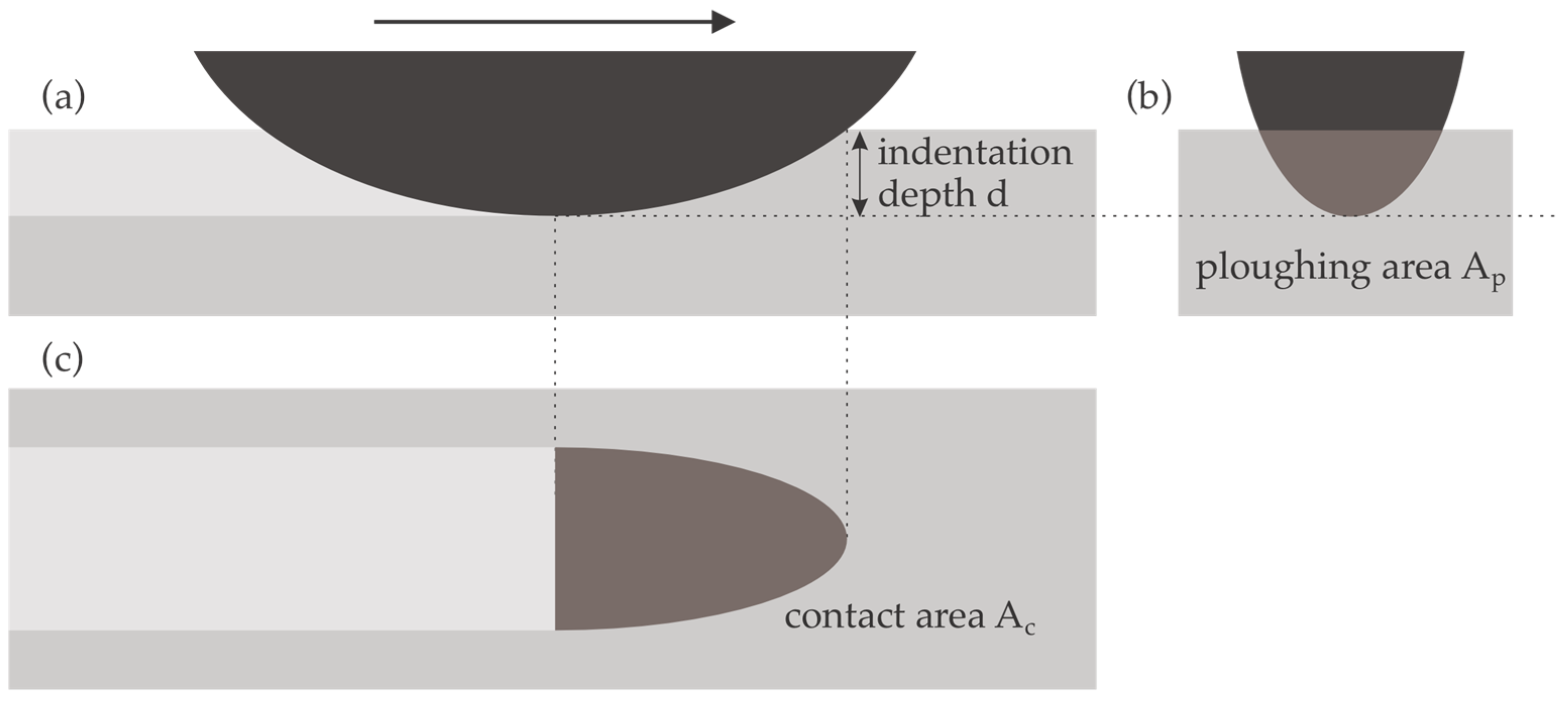
The plowing is assumed to remove the ice volume and, therefore, any rear part of the runner cannot come into contact unless it is located lower than any previous geometry features. From Figure 2, it can be seen that the contact zone will thus generally arise in the front part of the runner. For a spherical runner geometry on undisturbed ice, the resulting contact zone will be semi-elliptical when observed from above. In this stage, the plowing force is determined as

Figure 2.
Schematic side (a), front (b), and top (c) view of the plowing action of a simple loaded runner on an undisturbed ice surface inside the F.A.S.T. model. The indentation depth leads to geometrical overlap where ice material is plowed away in the contact zone. Both vertical load capacity and frictional drag from plowing are determined by the ice’s hardness and affected areas.
The plowing stage of the simulation results in the determination of the plowing force and the real contact area, i.e., the footprint of the runner on the ice.
The second stage calculates the thickness of the melt water layer under the consideration of heat transfer and Couette flow.
Consider a particular spot on the ice surface. It is assumed that a preexisting microscopical melt layer is always present on the ice surface (see, e.g., [8]). When the runner arrives, the available heat for the further melting of ice is calculated based on the following aspects.
- Generation of heat by shearing of the melt layer through its viscous properties
- “Slow” heat conduction from the ice surface into the bulk of the ice
- “Fast” heat conduction from the liquid melt layer into the ice surface
- Heat conduction from the runner into the liquid layer
The sum of these contributions produces the available heat. For any point on the ice, it is integrated over the sliding history from the first instance of contact and divided by the density and latent heat of fusion to determine the volume of melted water, i.e., the film thickness.
The longer a point on the ice is in contact, the greater its film thickness becomes.
From the film thickness h, the viscous resistance of the runner can be determined via integration over the contact zone:
Here, denotes the sliding velocity and the dynamic viscosity of water.
An interesting property of the model is that this second stage considers the geometry of the runner and ice only through the two-dimensional shape of the contact zone obtained in the plowing stage.
It should be noted that the F.A.S.T. model described by Poirier and Stell includes an additional procedure to calculate the effect of the squeeze flow out of the contact zone. This flow is directed sideways and reduces the film thickness. However, we found the effect of the additional calculation to be negligible in all relevant cases and have decided to disable it due to its high computation cost.
Furthermore, we would like to point out that the MATLAB implementation given by Stell contains flaws, which lead to inaccurate results. If you intend to work with this implementation, please consider our supplemental material in Appendix A.
2.2. Extensions to F.A.S.T.
Some of the restrictions of the original model make it unsuitable for realistically investigating in sports disciplines. We have extended the model to tackle the most relevant issues. In the following sections, we introduce the new requirements, discuss the implications that follow, and how we implemented them.
2.2.1. Generalizing Geometry
In the Poirier version of F.A.S.T., the geometries are always similar: the ice surface is perfectly flat and the runner is spherical with two radii of curvature. This configuration always leads to a semi-elliptical shape for the contact area, which is calculated analytically inside the program as a function of the indentation depth.
For arbitrary runner geometries, the area of contact is not generally accessible analytically and must instead be found by testing the surface pointwise: A value of the indentation depth is assumed and the entire runner geometry is lowered by that amount.
Then, each line of ice surface is traced from the front of the runner to the back, following the ice geometry. If the runner geometry intersects the surface, the latter is ploughed and the current position is marked as being in contact.
This must be performed for all rows and for each assumed indentation depth.
In order to satisfy Equation (1), the correct indentation depth must again be found iteratively. This process is straightforward but comes with considerable computational cost. In principle, any geometrical particularities of a given sport discipline can be accounted for.
For speed skating, the longitudinal blade radius and inclination angle of the blade are varied; for bobsleigh, the longitudinal geometry consists of a multitude of radii and the track is not flat. For a more detailed discussion of winter sport runner geometries, see the case studies in Section 3.1 and Section 3.2. Custom runner geometries can now be used and the track can be curved in both directions.
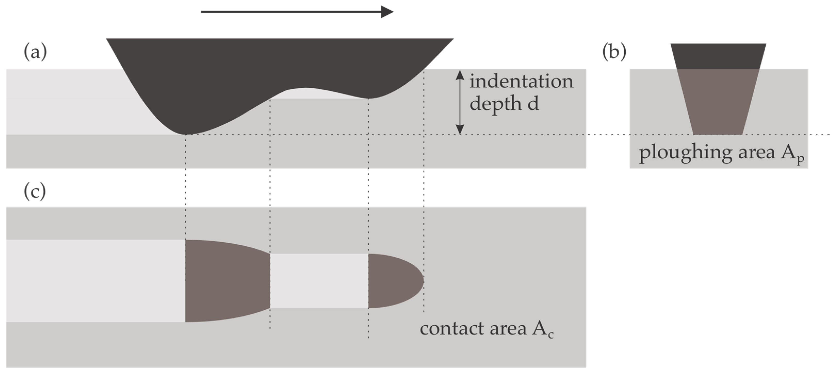
With arbitrary geometries, it can no longer be assumed that the resulting contact area is contiguous. Figure 3 shows an example.

Figure 3.
Schematic side (a), front (b), and top (c) view of the indentation configuration of an arbitrarily shaped loaded runner inside the improved F.A.S.T. model. The shape of the runner and the curvature of the ice can lead to multiple non-contiguous contact zones.
2.2.2. Refreezing of Liquid Layer
The non-contiguous contact areas have implications for the second stage of the simulation (film generation) as well. A point on the ice surface can enter into contact, leave contact, and come into contact again towards the rear of the runner.
The question arises of how the film thickness should evolve after the contact has been lost. Looking at the terms contributing to heat in the contact, it is clear that the heat from viscous shearing and from transfer related to the runner is absent when the ice is not in contact. The remaining terms are:
- “Slow” heat conduction from the ice surface into the bulk of the ice;
- “Fast” heat conduction from the liquid melt layer into the ice surface.
These correspond to some outflow of heat and, thus, the refreezing of the film after a loss of contact behind a runner contact section, see Section 3.2 for an example under real conditions.
2.2.3. Lateral Forces
For various disciplines, athletes rely on some lateral load to be carried by the runner, e.g., when passing through curves. We estimated the maximum load capacity in the y-direction by calculating the effective plowing area in the respective direction and multiplying it with the ice hardness. These values can differ between the left and right-hand sides when the runner/ice are tilted with respect to each other (for instance, in a turn inside a curved track).
2.2.4. Rotational Free Mounting of Runners
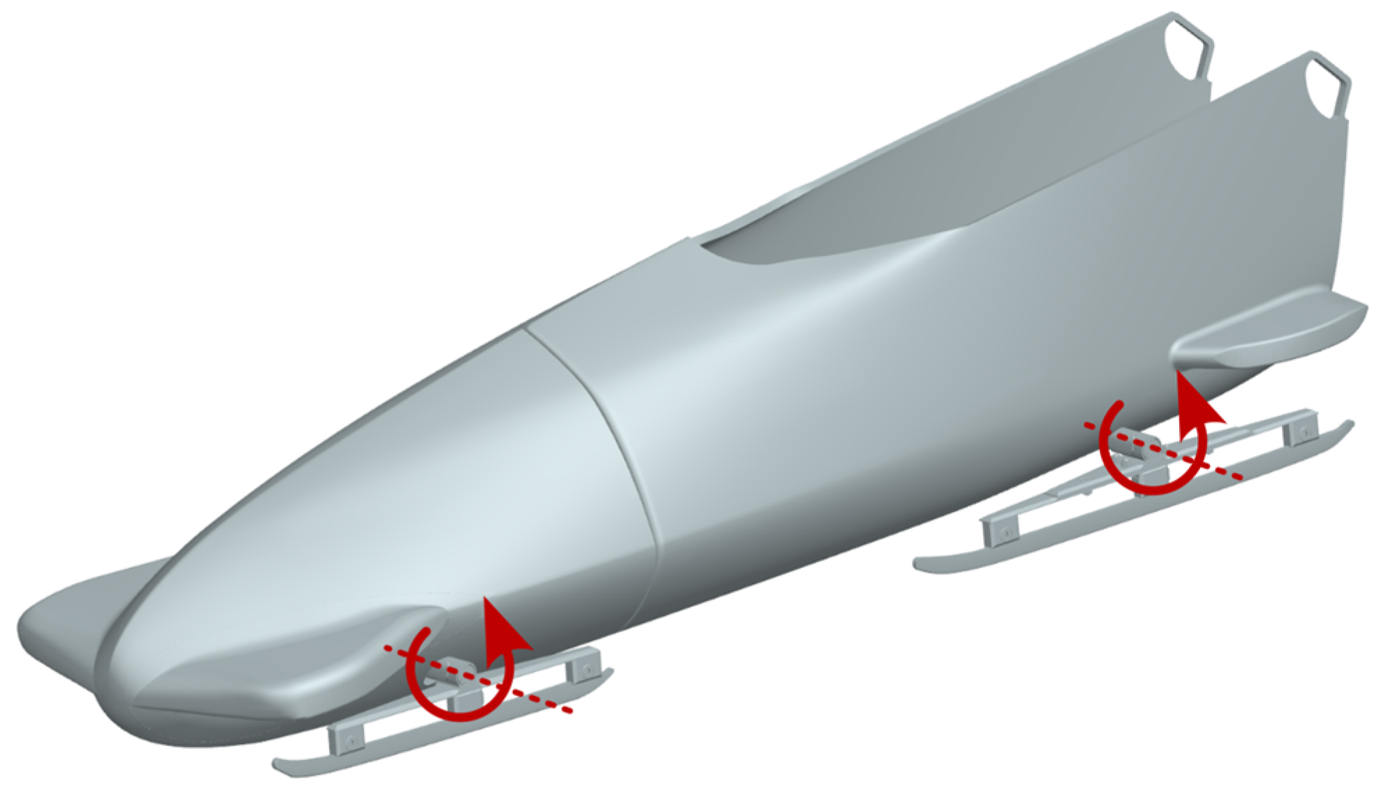
In the first stage of the F.A.S.T. model, the runner is lowered into the ice until the force balance is satisfied. The process is geometrically governed: an indentation depth is selected for which the resulting normal force is found to match the external load. However, the indentation depth is not the only geometrical parameter, even when 2D. The angle of attack also governs the footprint dramatically. For most applications, the angle of attack is not determined by the design of the sports equipment but rather a consequence of the load distribution front/rear on the runner or, more specifically, the absence of a rotational moment with respect to the y-axis. For speed skating, the point of reference can be understood as the athlete’s ankle joint. In bobsleigh, each runner has an individual fixed bearing to allow for a free adjustment of the angle of attack, see Figure 4.

Figure 4.
Typical mounting of bobsleigh runners. The runners are mounted in carriers, which have a rotational degree of freedom around the front and rear axle.
In order to account for this, the attack angle as an additional degree of freedom is introduced as well as the additional condition; therefore, the torsional moment, with respect to a given point , vanishes:
Numerically, a combination of the indentation depth d and the attack angle must be found iteratively to satisfy both Equations (1) and (4). This is numerically challenging for two major reasons.
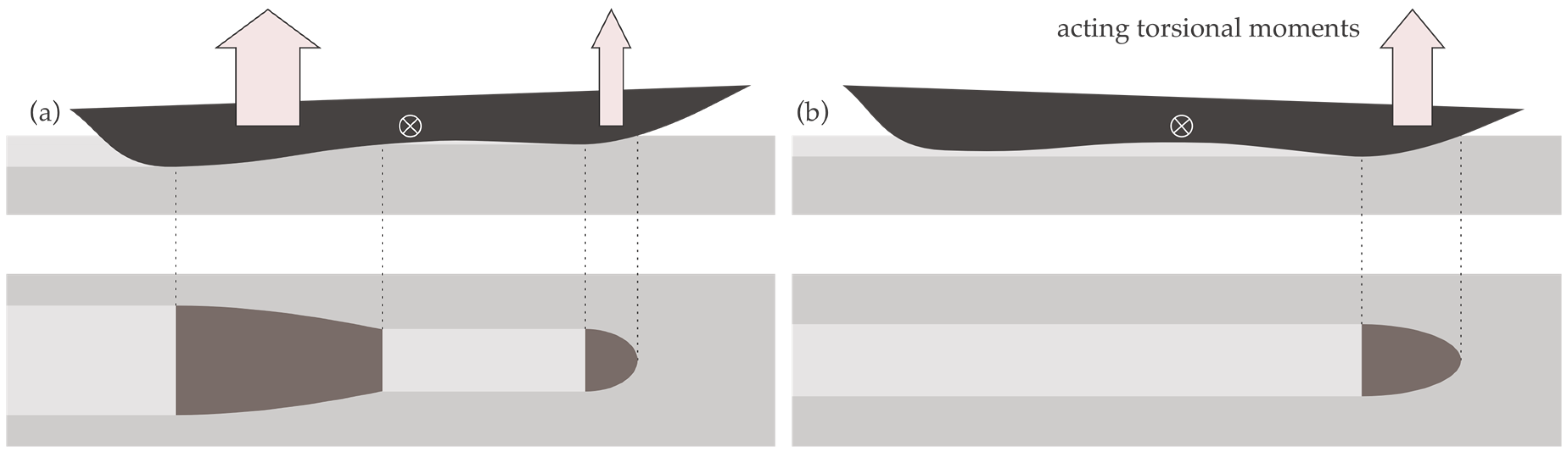
Firstly, the resulting normal force and even more so the resulting rotational moment are extremely sensitive to even the smallest adjustments of the selected values for the angle of attack and, to a lesser degree, to the indentation depth, see Figure 5.
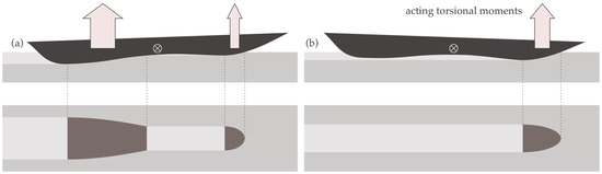
Figure 5.
In elongated runners, a slight change in the angle of attack will strongly affect the resulting footprint (compare (a) and (b)). Its influence on the position and value of the normal forces (arrows) and the resulting rotational moment around the lateral axes (circle with interior cross) is, therefore, extremely pronounced.
Secondly, since the computational domain consists of discrete elements, the contact area (multiplied by the ice hardness) cannot be tuned to match the normal force exactly. Instead, only discrete values can be obtained that correspond to a certain number of surface points identified to be in contact.
Again, for the determination of the resulting rotational torque, the discreteness of the contact area applies, preventing Equation (4) from being satisfied exactly. Both the indentation depth and the angle of attack must thus be chosen to represent a contact configuration (e.g., a subset of surface points to be in contact) which is a viable compromise in both equations.
As a consequence of the discrete nature of the problem, the dependencies are non-smooth and, therefore, cannot be tackled with standard optimization techniques.
In practice, we found this task to be the most challenging, with convergence towards a good compromise being very hard to achieve.
3. Results
The extensions made to the code hold many new possibilities and enable more realistic investigations of the friction behavior of winter sports equipment. As the first case study, we looked at several issues from the sports of speed skating and bobsleigh.
3.1. Speed Skating
As a first case study, we applied the extended F.A.S.T. implementation to the sport of speed skating, which the code was originally developed for.
Our advanced implementation of the F.A.S.T. code for speed skating allows not only for the realistic representation of loads and inclination angles but also for the advanced representation of realistic blade geometries. For example, modern speed skating blades do not only have a longitudinal radius (see in Figure 6) but also a pre-formed lateral radius, where the blade is bent around the vertical z-axis, to allow for better performance in the curves, additionally, the longitudinal geometry does not have to consist of a single radius, but can now be defined by a set of coordinates, which is essential and common for the discipline of short track, which uses variable radii over the length of the blade. Exploration of these variations in geometry will be conducted in future studies.
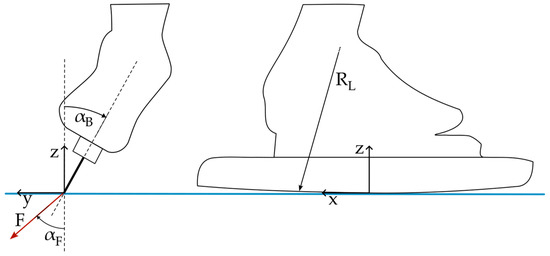
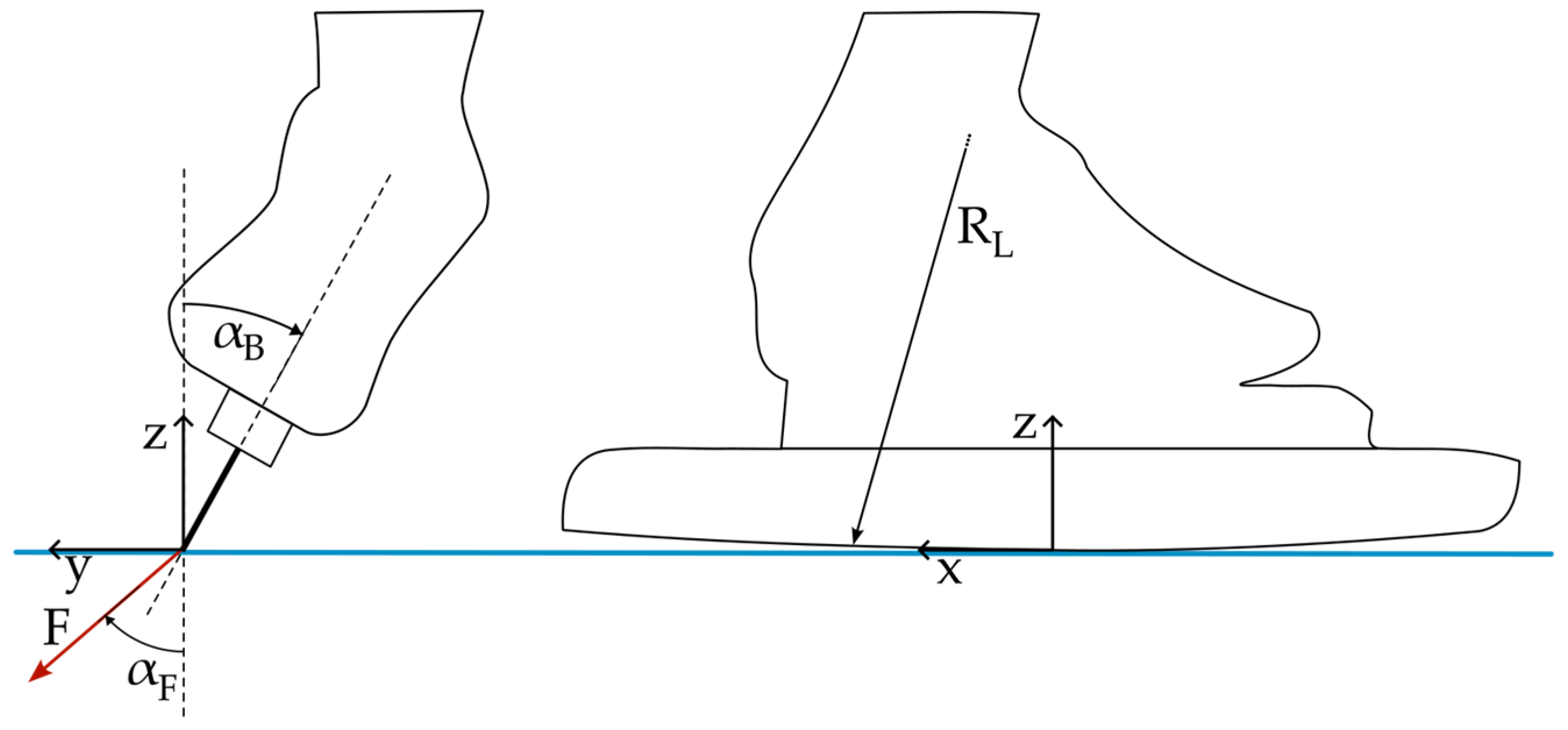
Figure 6.
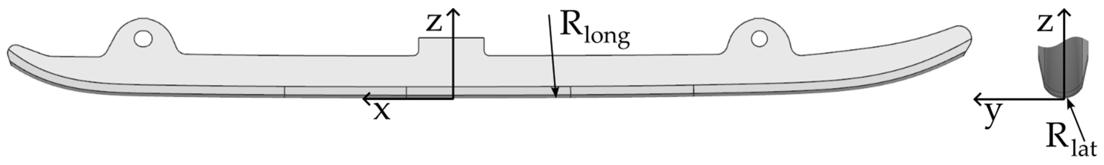
Sketch of a speed skating skate, consisting of a shoe, mounting system, and blade, from the front (left) and the side (right) with a coordinate system. The angle is the inclination angle of the blade, F is the total force acting on the ice, is the angle of attack of the force F and the radius is the longitudinal radius defining the blade geometry (note that the radius is sketched in an exaggerated manner). The blue line represents the ice surface.
Moreover, for basic speed skating geometries defined by only one longitudinal radius , the effect of an inclined blade on the geometry in relation to the ice has to be considered. When a blade with one longitudinal radius is inclined in relation to the ice, two things will happen. Firstly, the projected curve of the blade in the x–z-plane will not be spherical anymore and will have a lower curvature than the original radius. Secondly, the projection of the inclined blade in the x–y-plane will have an effect on the contact which resembles a camber or curvature around the z-axis and has a steering effect. For visual representation of these effects see Figure 7.
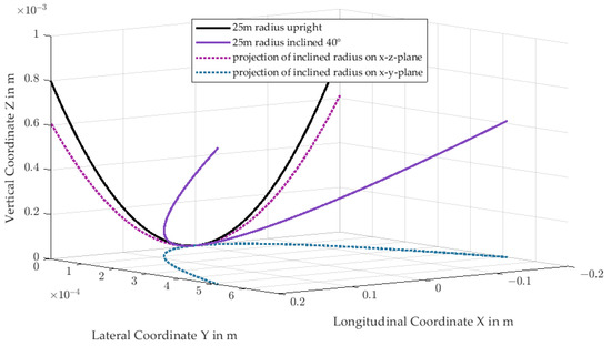
Figure 7.
Projection of a spherical curve after inclination. This graph serves as an aid to explain the effect of an inclined speed skating blade on contact geometry.
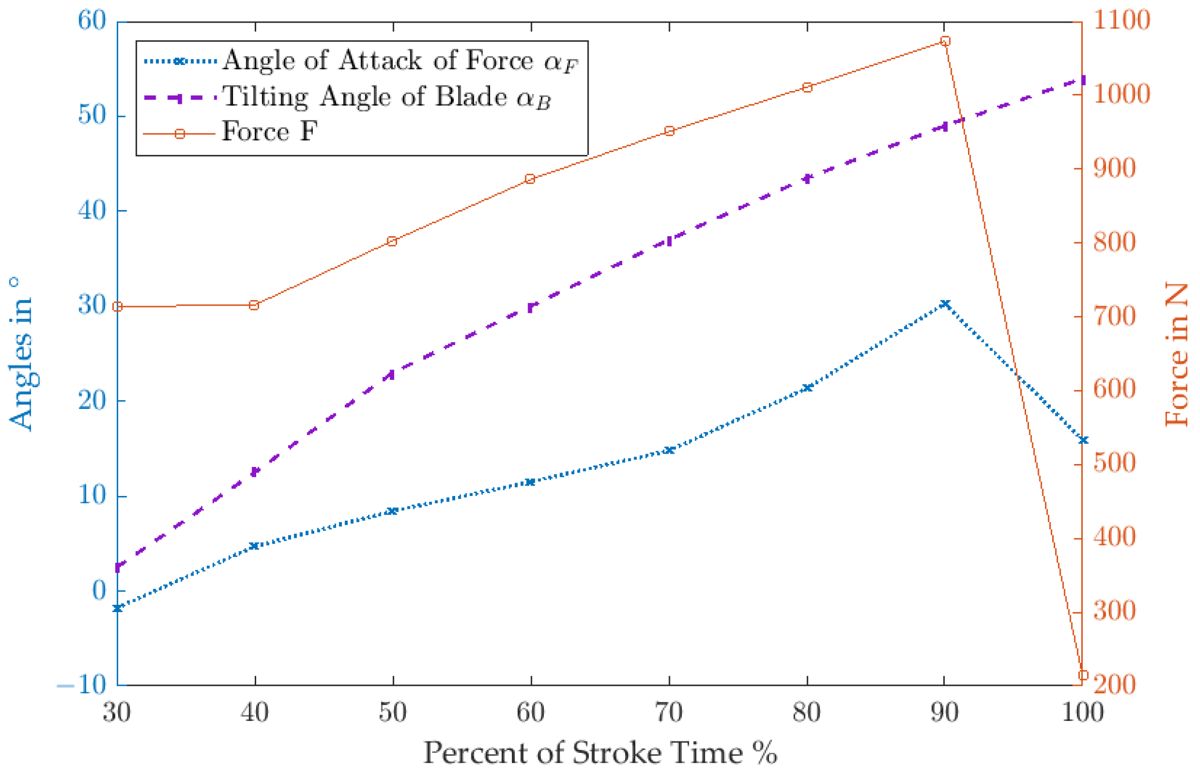
For our case study, we looked at the crucial part of the stroke cycle on the straightaway, using the measured forces and angles from [9,10] as they are shown in Figure 8. By using the region of 30–100% of the stroke cycle, we considered 80% of the total force per stroke and neglected the time of the stroke when both blades were in contact with the ice.

Figure 8.
Angles of force and blade (left vertical axis) and force onto the blade (right vertical axis) during a speed skating stroke on a straightaway, values derived from [9,10]. The angles are measured from the vertical axis in space.
For material parameters, we used the properties of a commonly used type of blade material, namely, powder metallurgical high-speed steel. If not stated otherwise, we used a standard blade geometry of a 25 m longitudinal radius , a skating speed of 8 m/s to comply with previous publications, and a standard ice temperature of −5 °C, which is common in speed skating arenas. A basal ice temperature 4 K below surface temperature was assumed as realistic based on interviews with technical staff.
As a first analysis, we calculated the development of the contact area over one stroke cycle (see Figure 9). Several effects can be observed in this analysis. Through higher inclination angles, the contact area becomes narrower, which is due to the sharper angles of the blade’s sides in contact. Simultaneously, the contact becomes longer, which is due to the fact that, by inclining a radius to the ice, the effective longitudinal radius increases (see Figure 7). This, again, leads to smaller indentation depths and, therefore, less plowing but also higher viscous drag due to the elongated contact. Depending on the relation between plowing and viscous contributions, the inclination can be beneficial to reduce overall friction.
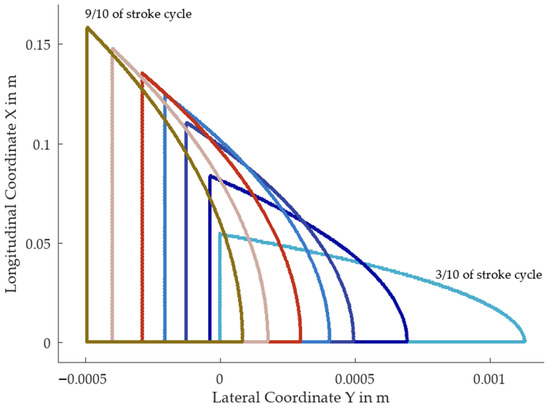
Figure 9.
Edges of contact zones for a speed skating stroke cycle on the straightaway with varying forces and angles, moving from the 30% point of the cycle (first contact area to the right in light blue) up to the 90% point of the cycle (most left contact area in olive green). The blade is moving towards positive x values or upwards in this graph.
It is also important to note that the edge of the blade is not positioned at the left edge of the contact area but starts at (0,0) and curves up to the first contact point. From this, the steering effect of an inclined blade can be easily understood, as the above-shown right blade runs on its inner edge (skating upwards) and has a tendency to steer to the left.
We performed calculations using variations in temperature in reference to the literature. For this analysis, we always calculated a “full” stroke cycle (meaning 30–100%) and calculated a mean coefficient of friction over the eight states. The results can be seen in Figure 10.
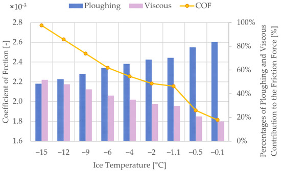
Figure 10.
Coefficient of friction of a speed skating stroke cycle for varying ice surface temperatures and otherwise standard values and the corresponding percentages of contribution from plowing and viscous forces to the total friction force. For ice temperatures above −1.1 °C, which is the melting temperature under pressure, the blade temperature was set equal to the ice temperature.
The biggest difference to previous results by Lozowski et al. [4] is the lower COF value and much lower sensitivity to changes in temperature. This is due to the fact that our algorithm calculates similar values of plowing force but much lower values of viscous forces than previous studies. The percentage contribution of viscous forces to the friction force is around 30–40%, whereas, in previous studies, it was found to be around 60–80%.
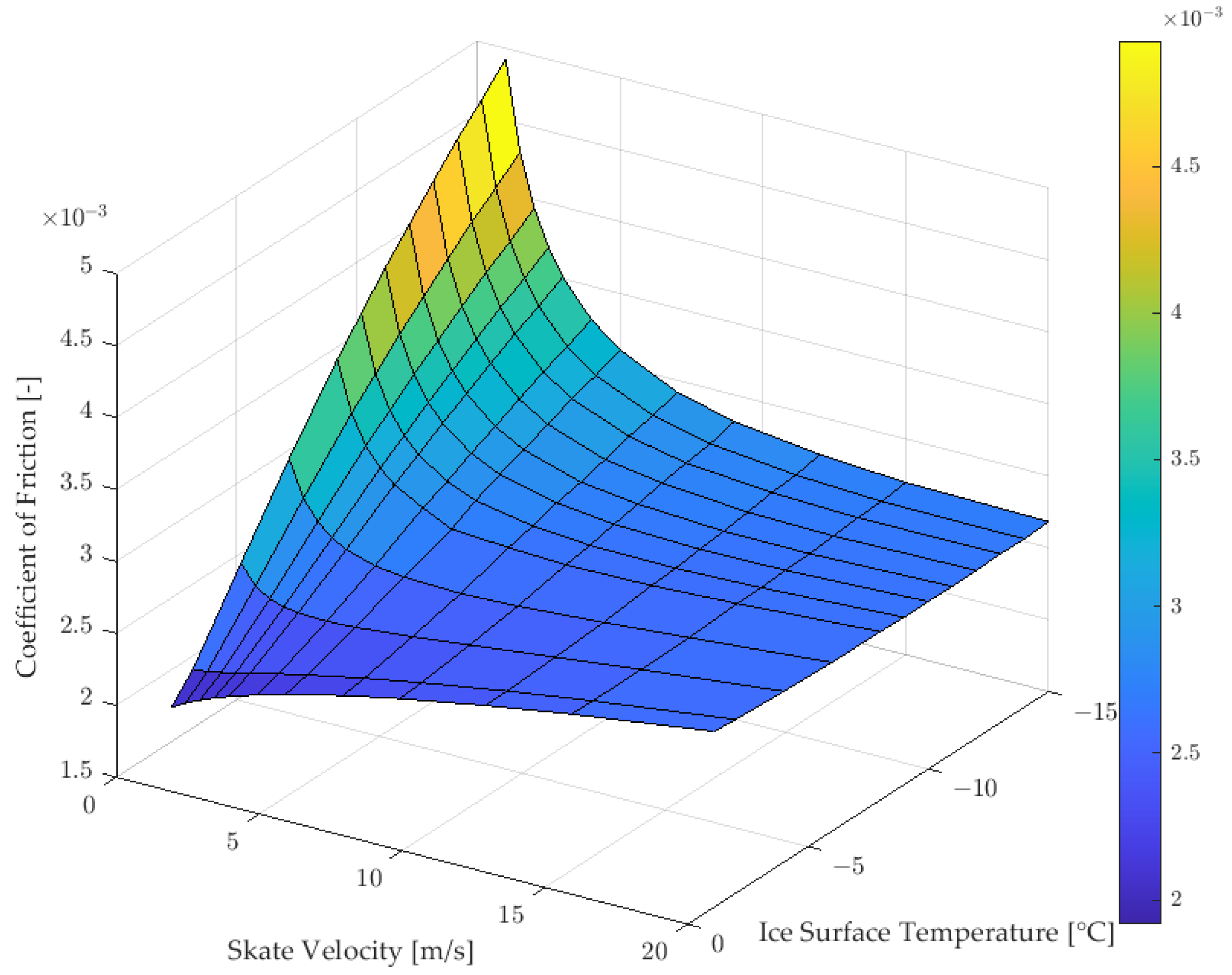
In the further analysis of different effects, the 60% point of the stroke cycle was chosen as a point of reference. For this state, an additional variation in skating speed was performed to investigate the sensitivity. The results can be seen in Figure 11 and show a similar behavior to the previous studies: the changes in ice temperature have a greater effect at lower velocities and with decreasing ice temperatures. The COF changes from rising with the rising speed at higher ice temperatures to falling with the rising speed at low ice temperatures.

Figure 11.
Coefficient of friction for the 60% point of the speed skating stroke cycle under variations of skate velocity and ice surface temperature.
When comparing our results to friction measurements in speed skating performed by de Koning et al. [11], two main things can be observed. Firstly, the coefficients of friction calculated using the algorithm are lower than the ones measured under realistic conditions. De Koning et al. measured COFs in the range of to under comparable conditions. This is partly explainable, as the algorithm neglects a few effects, e.g., imperfections and roughness of the ice surface and also the decelerating effects of active steering.
When looking at the more recent experimental results from Due et al. [7], which were obtained using a gliding vehicle, similarly higher COF values are measured. Secondly, the sensitivity of the COF to ice temperature and skating speed is much higher in de Koning’s measurements.
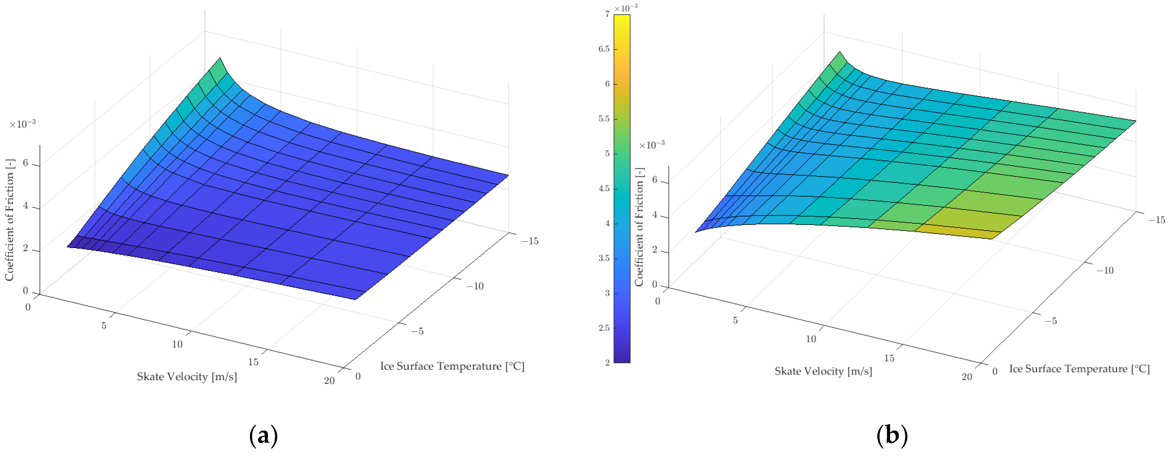
Both issues suggest that the algorithm underestimates the viscous forces. One possible explanation for this can be found when considering the research by Canale et al. [12]. Through friction experiments using atomic force microscopy with an ice surface, they found that the encountered viscosity of the melt water layer is much higher than the viscosity of water at 0 °C from the literature. The F.A.S.T. code uses the standard value of as dynamic viscosity , whereas Canale et al. calculated a complex dynamic viscosity with real and imaginary parts, with values for the real part in the range of to depending on temperature and sliding speed [12]. If the above analysis from Figure 11 is redone with a viscosity of , the results change considerably, not only in value but also in sensitivity to speed and temperature (see Figure 12).

Figure 12.
Coefficient of friction for the 60% point of the stroke cycle under variation of skate velocity and ice surface temperature with (a) dynamic viscosity of the water layer as in Figure 11 and (b) dynamic viscosity of the water layer in reference to [12]. Both (a) and (b) have the same axis limits and identical color ranges.
When we look at earlier publications for comparison, some research exists as a reference point, especially the publications [4,7]. However, due to a multitude of changes made to the code since then and further differences in the approach, we could not achieve comparability with these literature results.
3.2. Bobsleigh
As a second case study, the sport of bobsleigh was examined. Due to the above-mentioned additions to the code which allow for the definition of the blade or runner geometry through coordinates z(x) rather than a single radius, the calculation of real bobsleigh runner geometries becomes possible. Furthermore, the code now allows for curved ice surfaces, which allows the calculation of curves in the ice canal. In all ice canal sports, the loads are highest in curves and, therefore, the frictional losses are dominated by the curves.
The runner of bobsleighs can freely rotate around the lateral axis (see Figure 4). This is vital to maintain tangential contact with the ice while driving through curves. Our code is capable of delivering the angle of attack in equilibrium. As mentioned above, this addition comes with difficulties in convergence quality.
For a comparison of the overall behavior of the code in the sport of bobsleigh, we performed a variation over ice temperature and sliding speed using the following conditions.
For runner material parameters, we used Uddeholm Ramax HH, which is currently the only allowed material for bobsleigh runners. As longitudinal geometry, an older standard geometry of FES runners was used, which was developed in the early 2010s for the Altenberg track (see Figure 13). For lateral runner geometry, a radius of 7.5 mm is assumed, which is the allowed maximum and a common choice for two-man front runners. Concerning the normal force we assumed a mean normal acceleration on the sled of 1.4 g. With a total weight of 390 kg for a two-man bob and 44% of that load on the front runners (taken from [3]), we assume a load of 1220 N on a single front runner. For the track geometry, a mean curvature of a normal ice canal with a 90 m longitudinal radius and no lateral curvature is used. The sliding velocity was varied up to 35 m/s (126 km/h). These conditions are used as a standard for the bobsleigh analysis unless stated otherwise. For convergence reasons, we initially held the mounting rigid; therefore, we did not allow for a turning of the runner around the lateral axis, which is a valid assumption for open areas of the track (in contrast to narrow curves).

Figure 13.
Sketch of a bobsleigh runner geometry in side view (left) and front view (right, enlarged) with coordinate systems. The longitudinal shape of the runner surface is defined by a multitude of radii changing with coordinate x and a lateral radius , which may or may not change over x.
The field of the coefficient of friction, Figure 14, shows an overall similar picture to the speed skating results in Figure 11 but with lower values. The results are in general accordance with Poirier [3] but cannot be compared in detail, as Poirier usually calculates a front and a rear runner to obtain one value for a whole sled; however, he apparently adds both forces and applies them to one geometry. This is problematic due to two reasons: firstly, front and rear runners always have different longitudinal and lateral geometries and, secondly, as the relation between normal force and friction force is nonlinear, it is not the same to apply twice the load to one geometry as to apply once the load to two geometries.
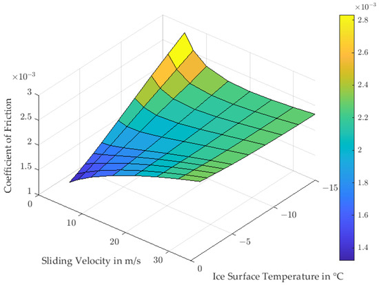
Figure 14.
Coefficient of friction of a 2-man bobsleigh front runner with rigid mounting under variation of sliding speed and ice surface temperature.
Comparing these results to practical experience from competitive bobsleighing highlights a few points. Firstly, the overall COF values are much lower than in reality. From energetic considerations, we know that the frictional losses during a bob run correspond to the mean frictional coefficient in the region of ~0.015. The difference in COF values is more straightforward in bobsledding than in speed skating, since the ice quality and ice surface quality of the ice canal is much lower than in a speed skating arena. The ice in the canal is rough, wavy, and sometimes damaged, which will add to the coefficient of friction.
Secondly, we know from our experience in the sport that the COF variation with ice temperature shown by the model is faulty: “warm” ice, which is close to its melting point, makes horrible conditions for the sport, as warm ice makes a track slow. Additionally, warm conditions lead to high wear of the ice and as a result the high-speed loss of the track during one heat, which leads to a dependence of the starting order on finish time. If possible, such conditions should always be prevented using more freezing power. This means the insensitivity to temperature at higher sliding speeds cannot be found in real bobsleigh conditions.
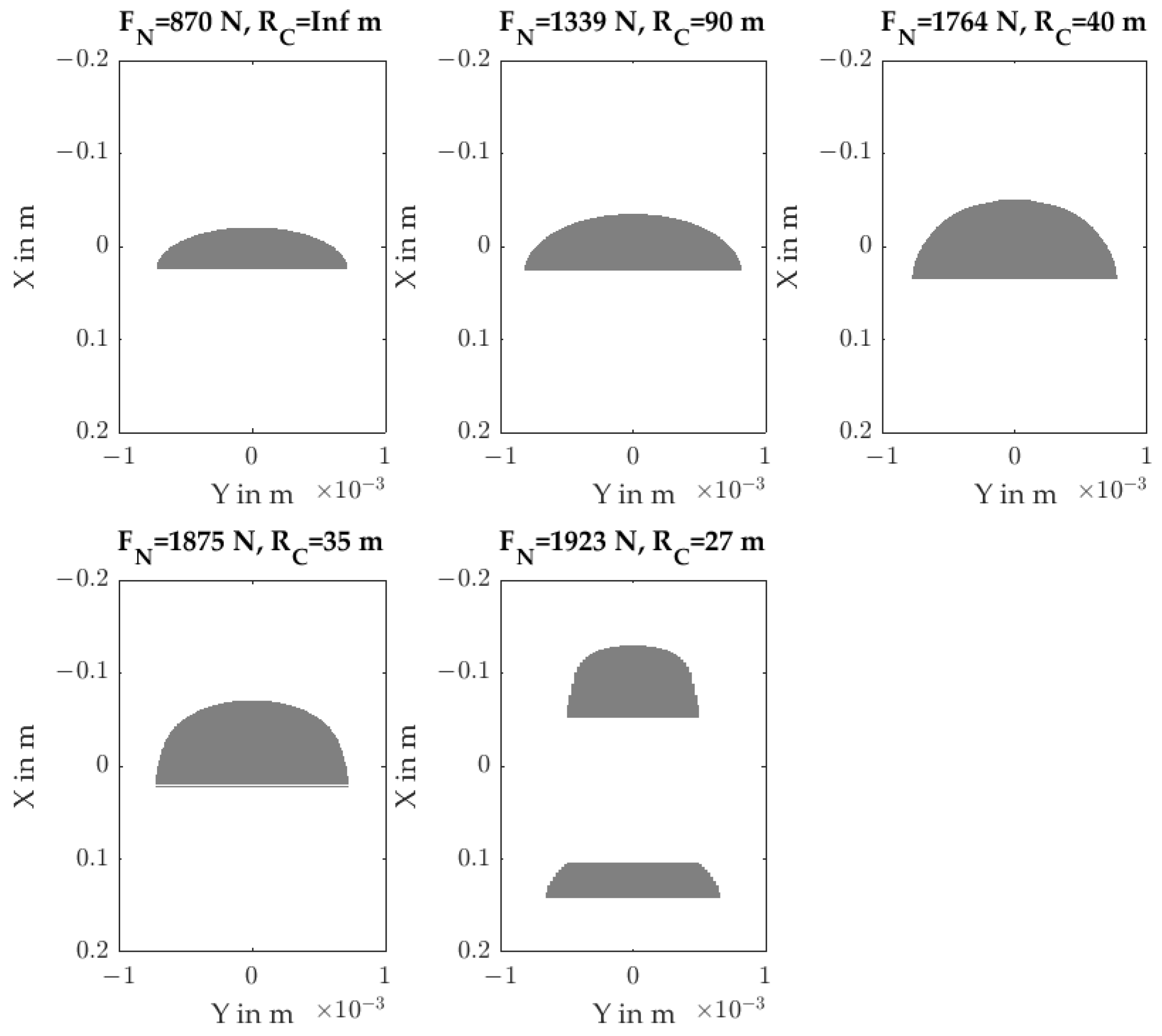
As a second bobsleigh case study, we looked at entering narrow curves, as these are always critical situations in a bobrun. There is a fast change in contact geometry, a high risk of drift, and a fast-changing normal load. When passing through narrow curves with flat runners, two separate contact areas can develop. Poirier already expected this behavior and mentioned the need for a corresponding extension to the model. But this is only now relevant, as real runner geometries can be calculated, because it is in curves, where the complex geometry of real runners comes into play. For this exemplary study, we looked at the entry into the spiral of the Yanqing National Sliding Center in the Beijing region, where the 2022 Winter Olympics were held. Over a 10 m distance, the track bends from straight to a curve of a 27 m radius, the normal load more than doubles, and the sliding speed is ~32 m/s. For the five intermediate states of this entry, we calculated the contact situation using the above-mentioned conditions, except for speed and ice temperature, which was held at −4 °C. For this analysis, the rotation of the runner was left free.
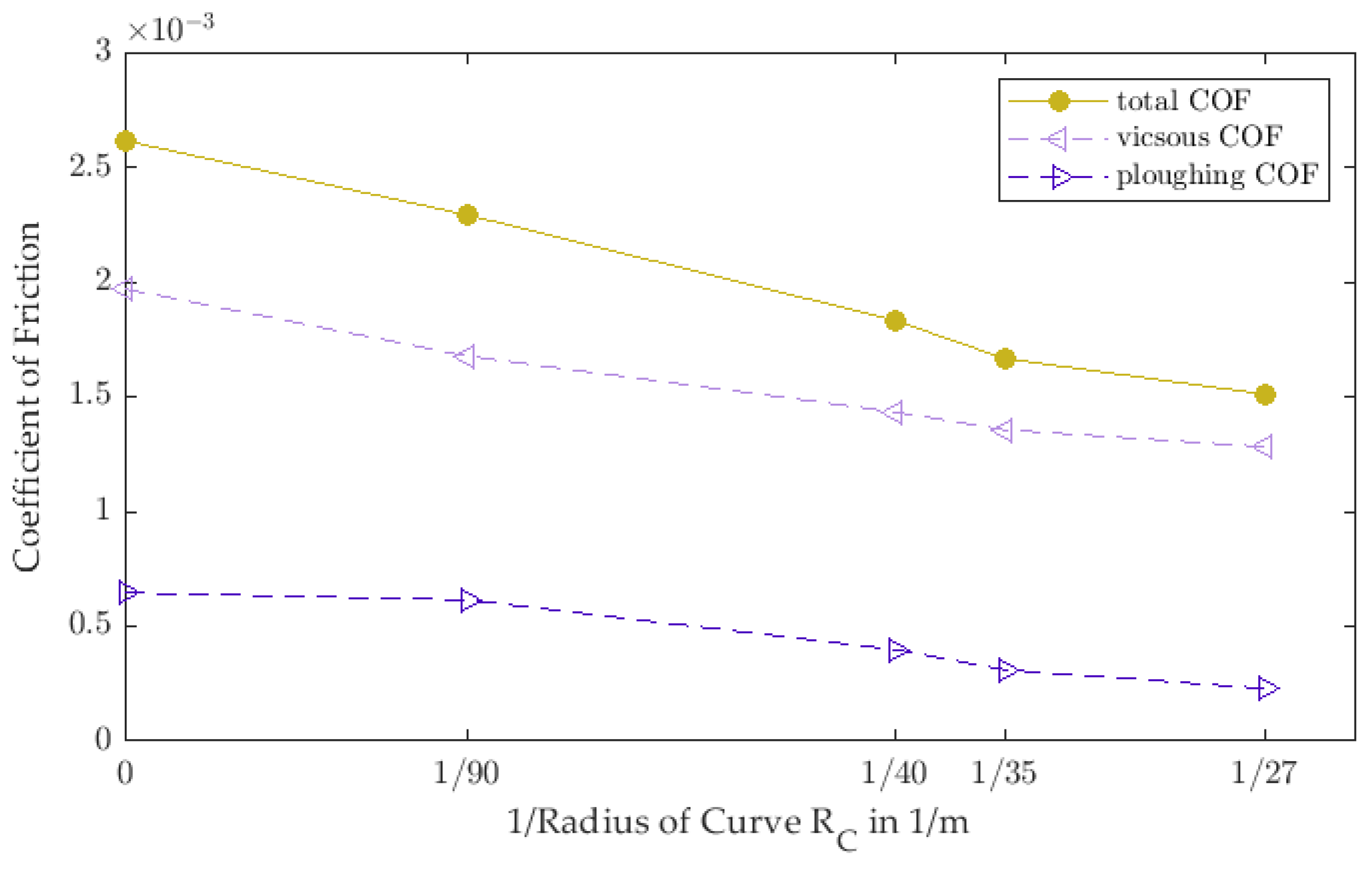
The results of the contact area in Figure 15 show that the code indeed can find equilibrium conditions with two separate contact areas, which do not have to be equal in size but in rotational equilibrium. We also see that during the entry into the curve, the contact area becomes longer rather than wider. This aligns with the results for the coefficient of friction, which decreases during entry into the curve as seen in Figure 16.

Figure 15.
Change in contact area while entering a curve in the track, decreasing curve radius, and increasing normal forces from top left (straight) to bottom right (final curve radius). The runner moves in the direction of negative x values (upwards).
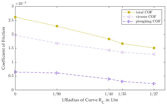
Figure 16.
Development of the coefficient of friction for a 2-man front runner while entering into a curve of 27 m radius. The values corresponding to plowing and viscous force are also shown.
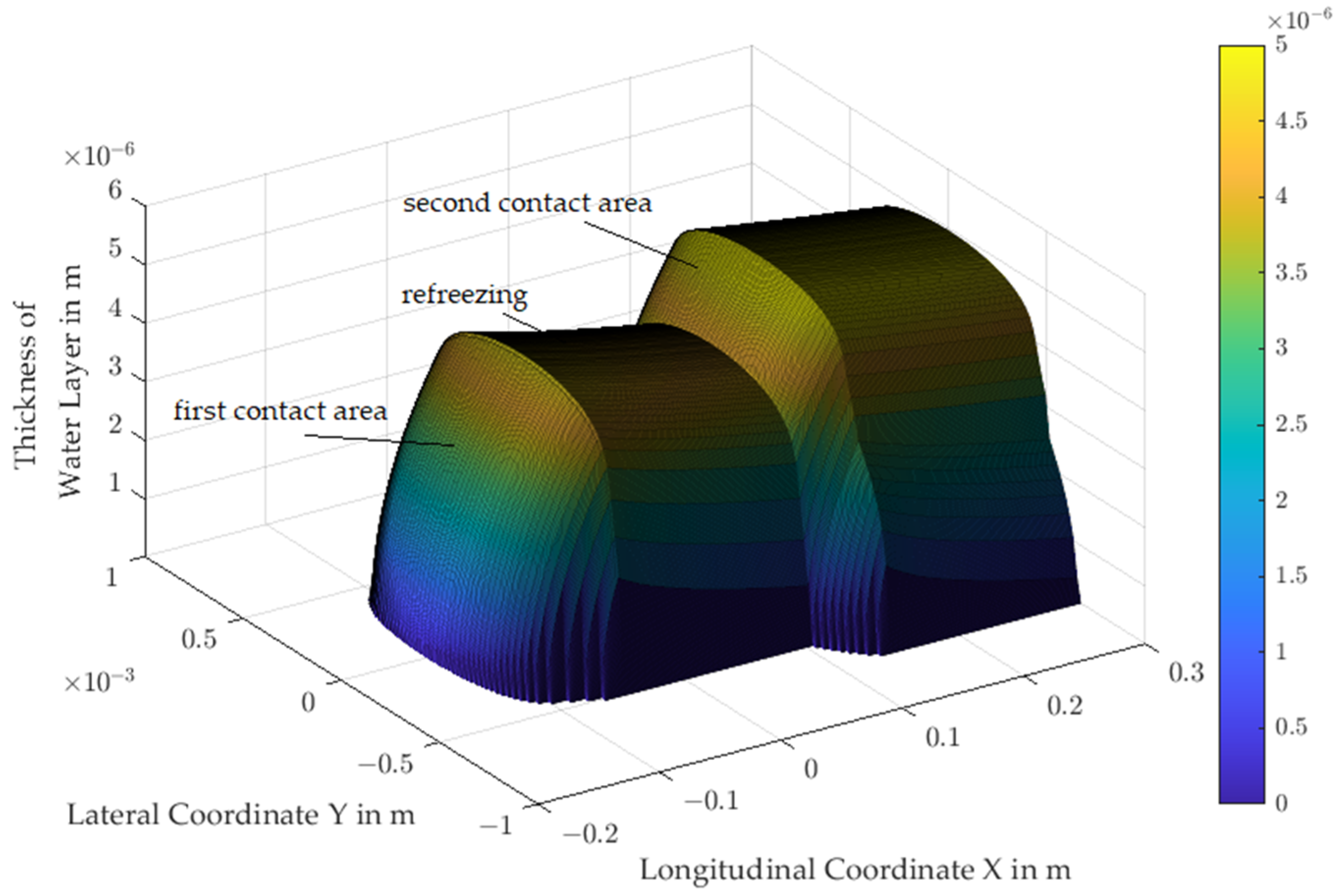
For this example, it is interesting to look at the development of the lubricating water film, which is depicted as a 3D plot in Figure 17 for the last calculated state of the curve entry. This last state is especially suitable to show the development of the melt water layer as it is a two-area contact. The figure shows how meltwater builds during the first contact. Between the two contacts, the melt water layer is preserved but slowly decreases in height as parts of it refreeze. Then, during the second contact, more ice is melted and the water layer increases again. This additional buildup leads to higher water layer thickness during the second contact compared to the first. Behind the second contact, the refreezing starts again and the water layer thickness decreases. In regions far behind the contact, the water layer will be refrozen completely (this region is not depicted in Figure 17).

Figure 17.
A 3D depiction of the water layer thickness for a 2-point contact as it occurs in narrow curves of the track (see Figure 15, bottom right). During passing, the water film increases and decreases again afterward. The runner moves in the direction of negative x values.
Furthermore, we looked at another specific issue derived from bobsleigh practice, which is a question of the effect of geometry. Poirier [3] determined that the F.A.S.T. code calculates much higher reductions in COF through flatter runners (i.e., a reduction in longitudinal radius) than from broader runners (i.e., an increase in lateral radius). Depending on the thermodynamic conditions, increasing the lateral radius can even increase friction in the model. This is because increasing the lateral radius reduces plowing but increases viscous forces and, depending on the other system conditions (temperature, velocity, and so on), one effect overweighs the other. This also highly depends on the normal load, as increasing normal loads increases the proportion of the plowing force. For high loads, e.g., 4 g of normal acceleration as in a curve, the gain through broader runners is higher, but still almost negligible compared to the gain through flatter runners.
This is another point where every person involved in the sport of bobsleigh would disagree because broader runners are found to be always faster given that there is no snow or hoarfrost on the track.
Whereas the use of flatter and broader runners is known to reduce frictional losses, in ice canal sports, it must always be balanced with control over the sled. Especially in curve entries and exits, pilots must have sufficient lateral grip to steer the sled in these strategically crucial situations. Losing control over the sled or encountering excessive drift can lead to side contact (i.e., time loss), hurt the ideal trajectory, and can set the sled up for a crash. Therefore, it is the responsibility of trainers and pilots to take into account their driving abilities, experience on a track, and weather conditions when choosing runners.
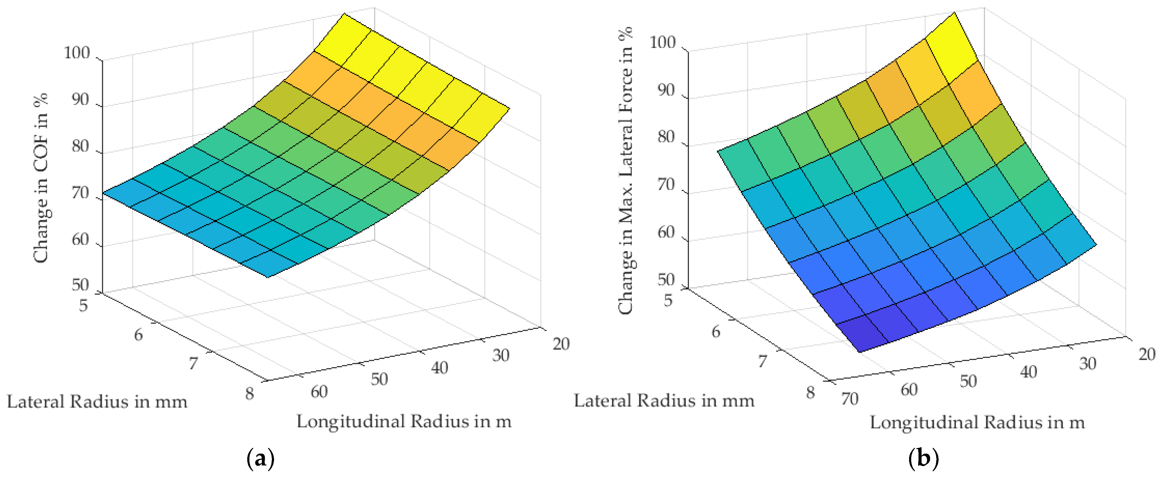
To get closer to a quantification of the control runners provide over a sled, we added the theoretically maximal lateral force the contact can hold as an output of the code. We did a variation of longitudinal and lateral radii over common ranges, now using a longitudinal geometry of one single radius. It can be seen in Figure 18 that increasing the lateral radius of the runner dramatically reduces the maximum lateral forces due to the decrease in indentation depth.

Figure 18.
Influence of changing the longitudinal and lateral radii of a bobsleigh runner on (a) the coefficient of friction and (b) the maximum lateral force. Only percental changes to maximum values are shown. Both (a,b) have identical axes and color scales.
Still, deducing from the model, one would always suggest choosing the flattest runners (limitations to this apply due to performance in narrow curves) and reducing the lateral radius if needed for control.
4. Discussion
With the new extensions of the F.A.S.T. code, a wide range of winter sport-specific questions can be investigated in a more realistic manner. In speed skating, the representation of correctly inclined geometries and lateral force components add significant benefits to move towards more realistic modeling of the sport. For bobsleigh applications, the implementation of free runner geometries and ice curvature makes the code much more realistic and usable for practicable application in the development of sports equipment. Adaptations for luge and skeleton are also possible and planned in the future. For luge, the new implementation of runner geometries is especially interesting, as the runners are mounted elastically with a camber; therefore, the contact geometry changes with the changing load as the runner turns around the x-axis. Moreover, for luge and skeleton, the implementation of free mounting is interesting, as the angle of the sled on the ice can be changed by the athlete through shifting weight.
Still, there are uncertainties in the implementation that should be further clarified through future research. This includes the ice hardness model, which was developed by Poirier [13] and recently reproduced by Du et al. [7] but is derived from measurements of drop tests with high scatter. The effect of deformation velocity on ice hardness, as well as the effect of pressure melting should be included in future ice hardness models. The publication by Liefferink et al. from 2021 [14] is an excellent starting point for this; however, it focuses on lower deformation velocities and is, therefore, not directly applicable. Furthermore, the temperature gradients in ice and blade are not well understood. The recent work by Du et al. [7] starts to tackle this issue, but due to the high sensitivity of the model to the blade temperature (as Poirier pointed out in [3]), a better representation could be beneficial, especially as we know in ice canal sports, the runner’s temperature has a high effect on finish time, and all runner temperatures are checked by officials before the start of the race. At last, with the work of Canale et al. [12], the viscous properties of the meltwater are under question.
All F.A.S.T. models in general produce coefficients of friction that are surprisingly low. From comparison with empirical values from winter sports, we would have assumed values higher by factors 4 to 6. In the ice canal sports, part of this discrepancy may stem from the waviness of the ice canal from scraping, which could be added to the model in the future for analysis. Furthermore, the consideration of surface roughness in the system is neglected by the model and shall be briefly discussed here. The slider roughness is relevant, as we know it can be of the same order of magnitude as the lubrication layer thickness. Measurements of the ice surface roughness and waviness in a winter sports context have not yet been published to the best of our knowledge. The implementation of ice surface roughness would bring additional challenges with it, as it would need a time-resolved simulation as the slider moves through the ice. It can be expected that a rough contact will show higher COFs, as the indentation depth and, therefore, the plowing force, as well as the viscous forces, due to a patchy lubrication layer, will be increased.
There are also a few other limitations to the code for the application in winter sports. A smaller possible addition for speed skating would be the implementation of a curved trace which is calculated from the steering effect of the inclined blade. The next big step towards a more realistic representation would be the consideration of the elasticity of the runners. It is known that speed skating blades under high inclination bend and, therefore, change their shape. This is due to the fact that the contact with the ice is usually in the middle part of the blade, whereas the force by the athlete is applied via two distributed mounts at the shoe, one under the heel and one under the ball of the foot. In luge and skeleton, the runners themselves but also the whole sled can bend and twist, especially in curves and curve entries and exits. Of course, the integration of elastic behavior into the model can have many possible forms and is a complex task that would not be easily accomplished.
Author Contributions
Methodology, Software, Formal Analysis, R.P.; Investigation, Project Administration, Funding Acquisition, B.G.; Conceptualization, Validation, Resources, Data Curation, Writing—original draft preparation, Writing—review and editing, Visualization, R.P. and B.G. All authors have read and agreed to the published version of the manuscript.
Funding
This research was funded by the Federal Ministry of the Interior and Community of the Federal Republic of Germany. Budget Section 0601, Budget Item 684 22.
Data Availability Statement
The code we base our work on is freely available in [6] with our suggested corrections in Appendix A. Requests to access the extended code or datasets should be directed to the corresponding authors.
Acknowledgments
We thank the FES project leads in the sports of speed skating and bobsleigh, M. Büttner, and E. Zinn, for providing discipline-specific data and information.
Conflicts of Interest
The authors declare no conflicts of interest.
Appendix A. Corrected Code from Stell
The appendix of Stell [6] gives specific implementations of his previous F.A.S.T. code in the MATLAB programming language. This implementation contains errors and should not be employed.
- Incorrect film thickness
When computing the film thickness, his code employs the following code segment a total of three times, either as dh or dhr:
| dh = dz*(… (u_w*v^2/h(i,j − 1)) … -(k_i*(T_i-T_b)/h_ice) … -(T_mf-T_i)*sqrt(v*p_i*c_i*k_i/(pi*abs(zo(i,1)−z(1,length(z))))) … +(T_sf-T_mf)*sqrt(v*p_s*c_s*k_s/(pi*abs(zo(i,1)−z(1,length(z))))) … )/(p_w*l_f*v); |
The corresponding formulae are numbered (2.29) and (2.30) in Stell [6], and, in Poirier [3], they are numbered (4.25) and (4.26). The error is in the usage (twice) of “z(1,length(z))”, which would give the coordinate at the end of the simulation domain. However, what is actually needed here is the running coordinate, as Poirier puts it, “The position along the length of the blade“. In the code, we need to instead insert “z(1,j)” and obtain
| dh = dz*(… (u_w*v^2/h(i,j − 1)) … -(k_i*(T_i-T_b)/h_ice) … -(T_mf- T_i)*sqrt(v*p_i*c_i*k_i/(pi*abs(zo(i,1)−z(1,j)))) … +(T_sf-T_mf)*sqrt(v*p_s*c_s*k_s/(pi*abs(zo(i,1)−z(1,j)))) … )/(p_w*l_f*v); |
This is consistent with the Python implementation of Poirier, which reads in the relevant section:
the code in question being “z0[j]-z” with decreasing “z -= dz”.
| for (k = 1;k<zsteps;k++) { z -= dz; h_condf = -dz * delta_T_i / (rho_w*l_f) *… …sqrt(k_i*rho_i*c_i / (v*pi*(z0[j]−z))); h_conds = dz * delta_T_s / (rho_w*l_f) *… …sqrt(rho_s*c_s*k_s / (v*pi*(z0[j]−z))); } |
- Missing case distinction for the contact area
There is an error in determining the contact area “A_r” of the rear runner when two runners are used. The Stell code reads on page 75 of [6]:
| A_r = (y_max+y_maxr)*l_sr; |
Which is only correct when both tracks overlap. Otherwise, the rear runner’s contact area is determined in the same way as the front runner (being “A_r = pi*y_maxr*l_sr/2”).
For the rear contact area, we thus need to discriminate between the two cases and write
| if m == 1 A_r = pi*y_maxr*l_sr/2; else % (being m == 0) A_r = (y_max+y_maxr)*l_sr; end |
References
- Penny, A.; Lozowski, E.; Forest, T.; Fong, C.; Maw, S.; Montgomery, P.; Sinha, N. Speedskate ice friction: Review and numerical model-FAST 1.0. In Physics and Chemistry of Ice, Proceedings of the 11th International Conference in the Physics and Chemistry of Ice, Bremerhaven, Germany, 23–28 July 2006; Kuhs, W.F., Ed.; RSC Publ.: London, UK, 2007; Volume 311, pp. 495–504. [Google Scholar]
- Lozowski, E.P.; Szilder, K. FAST 2.0 Derivation and New Analysis of a Hydrodynamic Model of Speed Skate Ice Friction. In Proceedings of the Twenty-First International Offshore and Polar Engineering Conference, Maui, HI, USA, 19–24 June 2011. [Google Scholar]
- Poirier, L. Ice Friction in the Sport of Bobsleigh. Ph.D. Thesis, University of Calgary, Calgary, AB, Canada, 2011. [Google Scholar]
- Lozowski, E.; Szilder, K.; Maw, S. A model of ice friction for a speed skate blade. Sports Eng. 2013, 16, 239–253. [Google Scholar] [CrossRef]
- Lozowski, E.P.; Szilder, K.; Maw, S.; Morris, A. A Model of Ice Friction for Skeleton Sled Runners. In Proceedings of the Twenty Fourth (2014) International Ocean and Polar Engineering Conference, Busan, Korea, 15–20 June 2014. [Google Scholar]
- Stell, B. Thermal-Fluid Dynamic Model of Luge Steels. Master’s Thesis, California Polytechnic State University, San Luis Obispo, CA, USA, 2017. [Google Scholar]
- Du, F.; Ke, P.; Hong, P. How ploughing and frictional melting regulate ice-skating friction. Friction 2023, 11, 2036–2058. [Google Scholar] [CrossRef]
- Döppenschmidt, A.; Butt, H.-J. Measuring the Thickness of the Liquid-like Layer on Ice Surfaces with Atomic Force Microscopy. Langmuir 2000, 16, 6709–6714. [Google Scholar] [CrossRef]
- van der Kruk, E.; den Braver, O.; Schwab, A.L.; van der Helm, F.C.T.; Veeger, H.E.J. Wireless instrumented klapskates for long-track speed skating. Sports Eng. 2016, 19, 273–281. [Google Scholar] [CrossRef]
- van der Kruk, E.; Schwab, A.L.; van der Helm, F.; Veeger, H. Getting the Angles Straight in Speed Skating: A Validation Study on an IMU Filter Design to Measure the Lean Angle of the Skate on the Straights. Procedia Eng. 2016, 147, 590–595. [Google Scholar] [CrossRef]
- de Koning, J.J.; de Groot, G.; van Ingen Schenau, G.J. Ice friction during speed skating. J. Biomech. 1992, 25, 565–571. [Google Scholar] [CrossRef] [PubMed]
- Canale, L.; Comtet, J.; Niguès, A.; Cohen, C.; Clanet, C.; Siria, A.; Bocquet, L. Nanorheology of Interfacial Water during Ice Gliding. Phys. Rev. X 2019, 9, 041025. [Google Scholar] [CrossRef]
- Poirier, L.; Lozowski, E.P.; Thompson, R.I. Ice hardness in winter sports. Cold Reg. Sci. Technol. 2011, 67, 129–134. [Google Scholar] [CrossRef]
- Liefferink, R.W.; Hsia, F.-C.; Weber, B.; Bonn, D. Friction on Ice: How Temperature, Pressure, and Speed Control the Slipperiness of Ice. Phys. Rev. X 2021, 11, 011025. [Google Scholar] [CrossRef]


Disclaimer/Publisher’s Note: The statements, opinions and data contained in all publications are solely those of the individual author(s) and contributor(s) and not of MDPI and/or the editor(s). MDPI and/or the editor(s) disclaim responsibility for any injury to people or property resulting from any ideas, methods, instructions or products referred to in the content. |
© 2024 by the authors. Licensee MDPI, Basel, Switzerland. This article is an open access article distributed under the terms and conditions of the Creative Commons Attribution (CC BY) license (https://creativecommons.org/licenses/by/4.0/).