Abstract
Micro-hole aerostatic bearings are important components in micro-low-gravity simulation of aerospace equipment, and the accuracy of micro-low-gravity simulation tests is affected by them. In order to eliminate the influence of air resistance on the attitude control accuracy of remote sensing satellites and achieve high fidelity of micro-low-gravity simulation tests, in this study, a design and parameter optimization method was proposed for micro-hole aerostatic bearings for a vacuum environment. Firstly, the theoretical analysis was conducted to investigate the impact of various bearing parameters and external conditions on the bearing load capacity and mass flow. Subsequently, a function model describing the variation in bearing load capacity and mass flow with bearing parameters was obtained utilizing a BP neural network. The parameters of aerostatic bearings in a vacuum environment were optimized using the non-dominated sorting genetic algorithm (NSGA-II) with the objectives of maximizing the load capacity and minimizing the mass flow. Subsequently, experimental tests were conducted on the optimized bearings in both atmospheric and vacuum conditions to evaluate their load capacity and mass flow. The results show that in a vacuum environment, the load capacity and mass flow of aerostatic bearings are increased compared to those in standard atmospheric conditions. Furthermore, it has been determined that the optimal solution for the bearing’s load capacity and mass flow occurs when the bearing has an orifice aperture of 0.1 mm, 36 holes, and an orifice distribution diameter of 38.83 mm. The corresponding load capacity and mass flow are 460.644 N and 11.816 L/min, respectively. The experimental and simulated errors are within 10%; thus, the accuracy of the simulation is verified.
1. Introduction
To ensure the operational precision of aerospace equipment, a micro-low-gravity environment needs to be constructed on the ground to validate the performance of the aerospace equipment, thereby comprehensively assessing various performance indicators of the aerospace equipment. In ambient pressure environments, it is challenging to achieve agile maneuvering and high-precision attitude control of remote sensing satellites due to factors such as air resistance [1]. In contrast, a vacuum environment can reduce the impact of the environment on micro-low-gravity simulation tests. Therefore, remote sensing satellites need to undergo testing in a vacuum to eliminate the effects of air resistance and other environmental factors on ground tests. As a crucial component in ground micro-low-gravity simulation for remote sensing satellites, the aerostatic bearings are essential to ensure the high fidelity of the experiments. Excessive air discharge from the bearings in a vacuum environment can adversely affect the level of the vacuum, thereby compromising the accuracy of ground-based micro-low-gravity simulation tests. However, the parameters of the bearings directly impact their performance. In order to design a micro-hole aerostatic bearing with a high-load capacity and low-mass flow in a vacuum, optimization of the bearing parameters is necessary.
Miyatake et al. [2] studied aerostatic thrust bearings with a diameter smaller than 0.05 mm, and the static and dynamic characteristics of the bearings were investigated using computational fluid dynamics (CFD) in comparison with those of composite throttling aerostatic thrust bearings. Gao et al. [3] examined the pressure distribution, load capacity, and stiffness of aerostatic bearings under various speeds and eccentric conditions, discussing the coupling of aerostatic and aerodynamic effects within the bearings. Chakraborty et al. [4] analyzed the performance of porous alumina film aerostatic bearings by combining theory and experiment under atmospheric pressure, and the results showed that the bearing bore diameter, air supply pressure, and radial load had a great influence on its performance. Khim et al. [5] analyzed the phenomenon of pressure increase in aerostatic bearings moving under vacuum conditions through theoretical analysis and experimental validation, attributing the pressure rise to additional leakage caused by stage velocity and air molecules adsorption and desorption from the guide rail surface. Fukui et al. [6] investigated the characteristics of externally pressurized bearings under high Knudsen number conditions at an environmental pressure of 0.1 kPa. Experimental results showed similarities with lubrication equation simulations, confirming the applicability of the lubrication equation. Trost et al. [7] studied small orifice throttling aerostatic bearings under vacuum conditions, determining the critical pressure and critical radius at which viscous air flows within the bearing transition to molecular flow and establishing the relationship. Schenk et al. [8] researched the characteristics of aerostatic bearings in a vacuum environment, observing a decrease in stiffness and an increase in load capacity compared to atmospheric pressure conditions, and proposed a flow field calculation model at any supply air pressure. Gan et al. [9] investigated the slip effect of air lubrication at arbitrary Knudsen numbers using the Boltzmann equation. These studies indicated that the performance of bearings in a vacuum environment differs from that in atmospheric pressure conditions, yet the lubrication equation remains applicable in a vacuum. Chan et al. [10] optimized the structure of bearings using a particle swarm optimization algorithm to maximize stiffness and minimize friction. Wang et al. [11] employed a genetic algorithm to optimize the structure of porous bearings to maximize load capacity and stiffness, enhancing computational efficiency. Nenzi et al. [12] optimized aerostatic bearings using the cubic partitioning method (HDM), demonstrating that the HDM method could obtain multiple optimal solutions with less computational effort. Yifei et al. [13] established mathematical models for stiffness and dynamic stability, conducted optimization calculations under different load conditions, and verified the optimization results. Hsin et al. [14] utilized the two-stage grid-interpolated fitting (GIF) method for bearing optimization design, obtaining a larger Pareto front distribution with reduced computational effort. Zhang et al. [15] studied the application of machine learning with neural networks and genetic algorithms in multi-objective optimization of heat exchangers, developing prediction models for heat transfer coefficients and pressure drops. By designing models with different parameters and training datasets, they utilized neural networks for prediction and employed multi-objective genetic algorithms for global optimization to obtain the Pareto boundary solution set for optimal combinations of key parameters. Few researchers have focused on optimizing bearing parameters based on mass flow, and optimization of aerostatic bearings parameters has mainly been conducted under atmospheric pressure conditions, thus lacking optimal parameters for bearings in a vacuum environment. In conclusion, there is a need to propose a design and optimization method for aerostatic bearings in a vacuum environment.
According to the aforementioned research, most scholars have focused on the study of aerostatic bearings in ambient pressure conditions, with limited research on bearing performance in vacuum environments. Furthermore, studies conducted in vacuum environments have only explored bearings under specific parameters, without providing principles for selecting and optimizing parameters for bearings in vacuum conditions. In order to mitigate the impact of air resistance on the precision of attitude control for remote sensing satellites, micro-low-gravity experiments and the use of bearings must be carried out in a vacuum. In a vacuum environment, the Reynolds equation is solved using the five-point difference method in this study. The effects of bearing parameters (air film thickness, number of orifices, aperture of orifice, and distribution diameter of orifice) and external environment (air supply pressure and vacuum level) on the load capacity and mass flow are analyzed. With the objectives of maximizing load capacity and minimizing mass flow, the target function is nonlinearly fitted using a BP neural network. The NSGA-II algorithm is then employed to determine the Pareto front optimal solution of the bearing in a vacuum environment. The optimal parameters of the bearing in a vacuum environment are obtained by applying the maximum–minimum value method to multiple sets of solution strategies. The accuracy of the optimization method is demonstrated through a comparison of numerical analysis and experimental verification. A comparison between numerical analysis and experimental verification demonstrates the accuracy of the optimization method, providing a theoretical and experimental approach for the application of bearings in vacuum settings.
2. Theory and Methods
2.1. Structure of Air Bearing
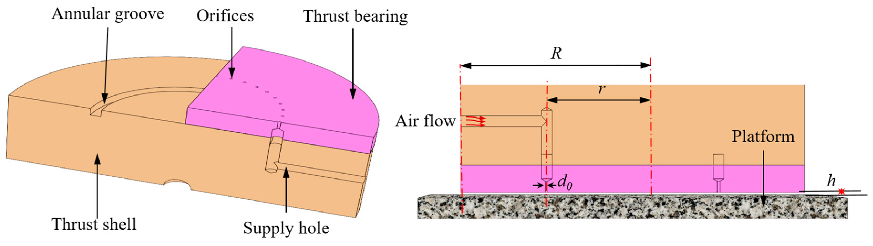
The structure of aerostatic thrust bearing is shown in Figure 1. The aerostatic thrust bearing mainly consists of the thrust shell and the thrust bearing. There is an annular groove on the thrust shell, and this structure allows for the air to enter from the supply hole to be uniformly distributed to the orifices of the thrust bearing. The outer diameter of the aerostatic thrust bearing is R; the distribution diameter of the orifice is r; the aperture of the orifice is d0, and the air film thickness is h. When the bearing is in operation, high-pressure external air flows into the annular groove of the thrust shell from the supply hole and then into the uniformly distributed orifices. Due to the pressure inside the air film thickness being higher than the external ambient pressure, the pressure difference between them generates the load capacity, causing the bearing to float.
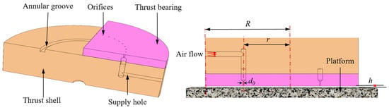
Figure 1.
The structure of aerostatic thrust bearing.
2.2. Theory Model
In the vacuum environment, the flow of air in the flow field satisfies the Navier–Stokes equations. Simplifying the flow field, the Reynolds equation for the stable flow of air in a thrust-bearing flow field is expressed as [16]:
Let , and the dimensionless Reynolds equation can be written as
where r is the radial length of the bearing; θ is the circumferential angle of the bearing; h is the air film thickness; p is the internal pressure of the air; η is the dynamic viscosity of the air; r0 is the reference radius; pa is the ambient pressure, and h0 is the reference film thickness. At the orifice , and at the non-orifice .
The mass flow of air outflow at the orifice is expressed as [16]:
where is the flow coefficient; is the air supply pressure; is the area of the orifice; and are the environmental pressure and atmospheric density respectively, and the air density in vacuum is
where is the density of air in the standard state; is the temperature of the air in the standard state; is the standard atmospheric pressure, and is the ambient temperature.
The flow function is represented as follows [16]:
where is the adiabatic coefficient; is the orifice outlet pressure, and is the critical pressure ratio. The mass flow of the air into the orifice should be equal to the mass flow out, as shown in Equation (6).
By solving the partial differential equation of Equation (2), the pressure distribution of the bearing can be obtained; the bearing load can be obtained by integrating the pressure against the bearing surface, and the mass flow of the bearing can be obtained by Equation (3).
2.3. Solution Algorithm
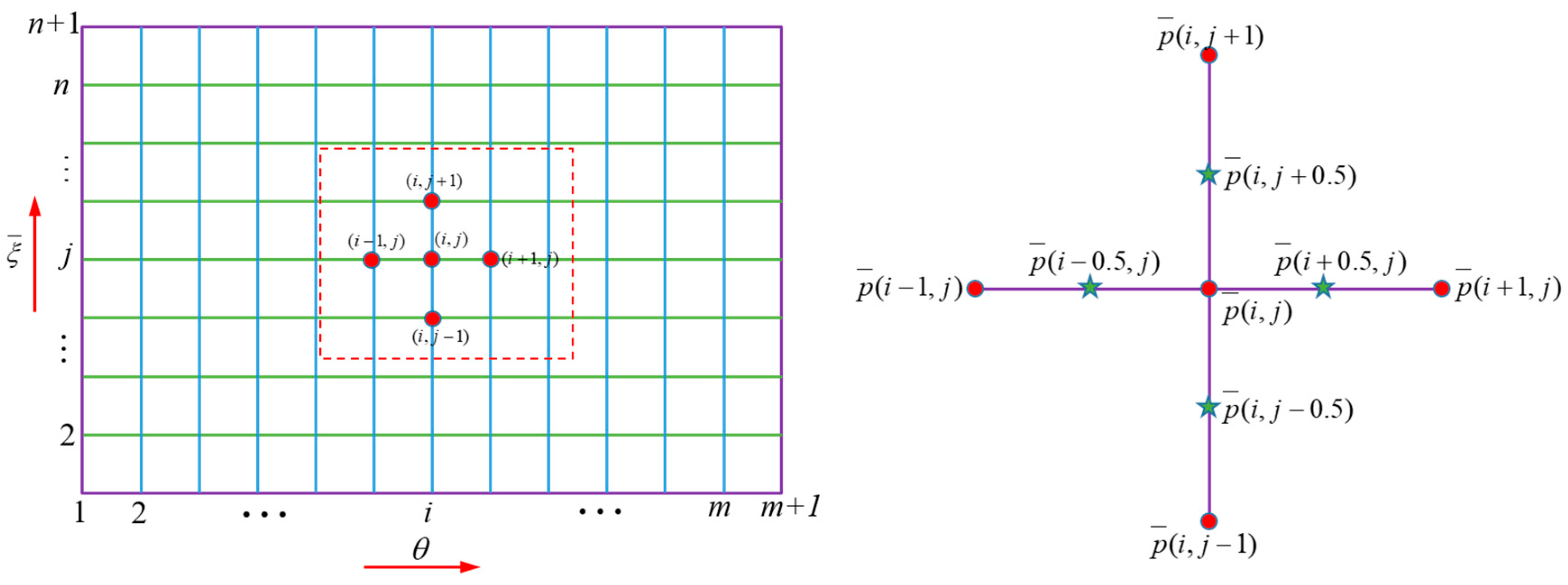
The finite difference method has the advantages of high precision and fast convergence, etc. Therefore, the finite difference method is used to solve the partial differential equation of Equation (2), and the solving process is shown in Figure 2. nodes are set in direction , and nodes are set in direction . The and boundaries are periodic boundaries, and the and boundaries are atmospheric boundaries.
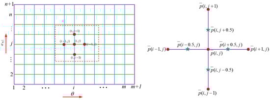
Figure 2.
Finite difference method.
Using the difference Equation and the pressure of neighboring points, is obtained as follows:
The coefficients in the Equation are expressed as follows:
The pressure is adjusted by Equation (9):
where is the adjustment coefficient and its value is 0 to 1; is the pressure of the previous iteration, and is the pressure of the next iteration. The iteration stops when the difference between the two is sufficiently small. Based on the above methods, calculate the pressure distribution of the bearing and obtain the bearing capacity and mass flow as follows:
2.4. Optimization Method
According to Equation (10), it can be obtained that the bearing capacity and mass flow vary with the position, quantity, and diameter of the bearing orifices. In order to achieve high bearing capacity, a greater number of orifices and a larger mass flow are required, resulting in coupling between variables. Therefore, in order to obtain a bearing structure with high bearing capacity and low mass flow, it is necessary to establish the functional relationship between bearing capacity and mass flow concerning the number, diameter, and position of the orifices. By identifying its relative minimum value, the optimal solution can be obtained.
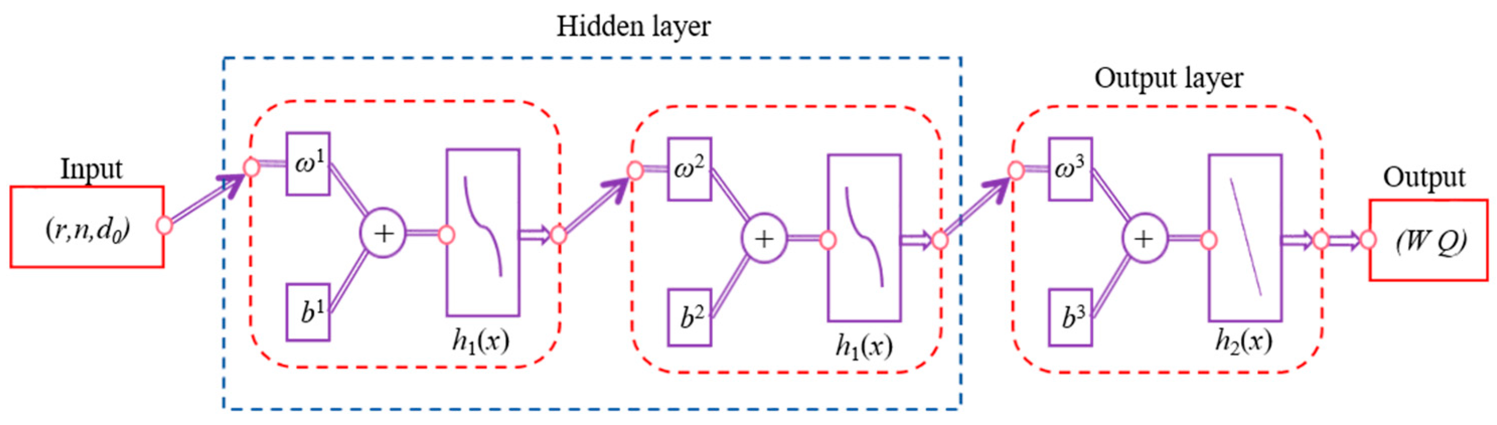
As a nonlinear fitting algorithm, the BP neural network can process and fit complex functional relationships with strong applicability. Therefore, the BP neural network is chosen to fit the model [17,18]. The constructed neural network is shown in Figure 3. The input layer consists of three variables, namely, the distribution circle radius r, the number of orifices n, and the aperture of orifice d0. Two hidden layers are selected for nonlinear mapping, and the output layers are bearing capacity and mass flow.
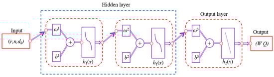
Figure 3.
BP neural network structure.
The weights and biases obtained from the training of the BP neural network are passed through the transfer functions of the hidden and output layers, which then undergo nonlinear mapping to ultimately derive the output results. These output results are compared with the actual target values to calculate the loss function. Finally, adjustments are made to the parameters through the backpropagation of the neural network. The training of the neural network stops when the sum of the overall error squares is minimized.
Given the input variable , the weights and biases of the hidden layer are denoted as , , , , with the activation function of the hidden layer being . The weights and biases of the output layer are represented by and , with the activation function of the output layer being . According to the principle of the BP neural network, the output of the output layer can be expressed as
The determination coefficient is usually used to judge the fit degree, as shown in Equation (12). In this equation, is the predicted value of the objective function; is the true value of the objective function; is the average value of the objective function, and is the determination coefficient. The closer the determination coefficient is to 1, the better the fitting effect is proved.
According to Equation (11), the relationship between bearing capacity and mass flow as functions of the position, quantity, and diameter of the bearing orifices can be obtained. This represents the optimized model, as shown in Equation (13). , , and represent the minimum values of design variables, while , , and represent the maximum values of design variables, with being the objective function.
The non-dominated sorting genetic algorithm (NSGA-II) is a multi-objective optimization algorithm based on domination [19,20], which can obtain better optimization results when solving complex multi-objective optimization problems. In this paper, the NSGA-II algorithm is used to optimize the structure of bearings to obtain multiple sets of Pareto front optimal solutions [21]. Subsequently, a decision is made on the multiple sets of Pareto front optimal solutions based on Equation (14) [22], leading to the ultimate determination of the optimal bearing parameters.
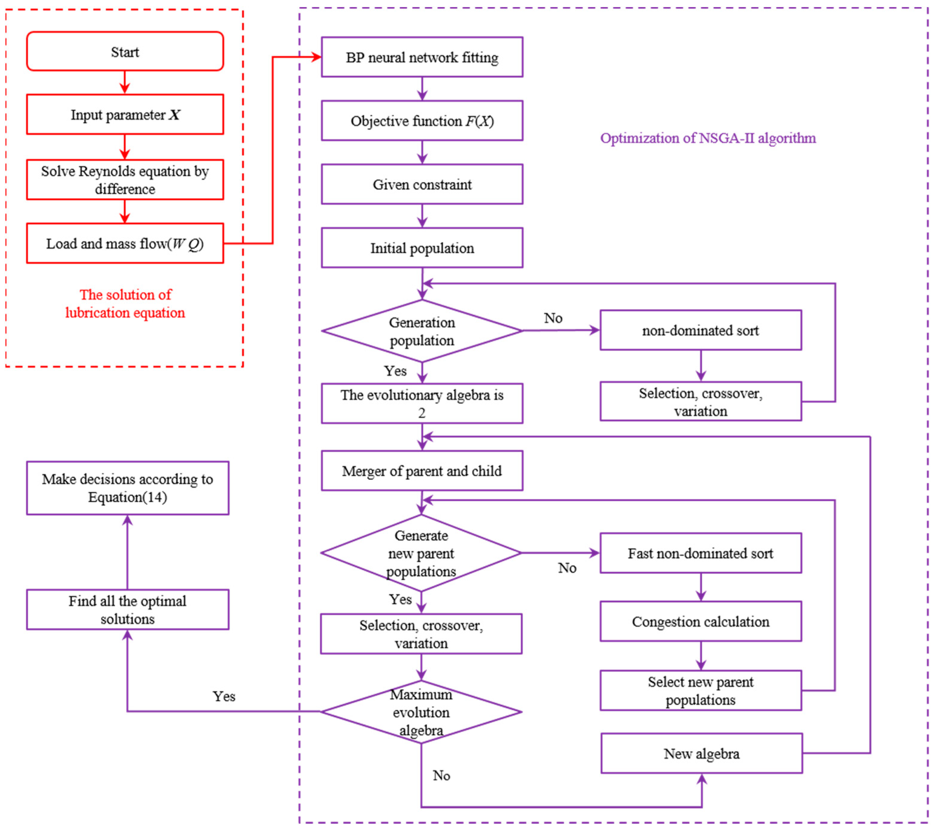
where and are the deviation of bearing capacity and mass flow from the optimal solution; is the size of bearing capacity in the Pareto frontier optimal solution, and is the size of each mass flow in the Pareto frontier optimal solution. , , , are the maximum and minimum values of bearing capacity and mass flow in the Pareto frontier optimal solution. By calculating from Equation (14), the optimal bearing capacity and mass flow of the bearing under vacuum can be obtained, and the corresponding solution is the optimal design parameter of the bearing. The calculation process is shown in Figure 4.
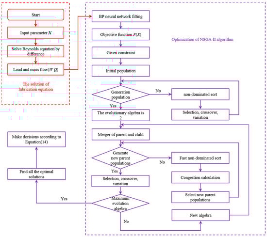
Figure 4.
Calculation flow chart.
The solution process is as follows:
- 1.
- Input bearing parameters (distribution diameter of orifice, number of orifices, aperture, etc.) and solve Reynolds equation according to Equations (1)–(9) to obtain pressure distribution;
- 2.
- According to the pressure distribution, the bearing capacity W and mass flow Q are solved according to Equation (10);
- 3.
- The objective function F(X) is obtained by using the BP neural network and Equation (11);
- 4.
- Constraints of the independent variables are given, and the population is initialized;
- 5.
- Select, cross, and mutate the population, then perform non-sequential sorting to obtain the next generation of the population;
- 6.
- Merge the offspring and parent populations to form a new population, then conduct a fast, non-dominated sorting, calculate crowding distance, and rank the population based on non-inferior levels;
- 7.
- Repeat the process of selecting, crossing, and mutating the population, then evaluate if the evolutionary generation criteria are met; if so, output the results; if not, continue the process until the criteria are met;
- 8.
- Make decisions on multiple solutions to obtain the optimal bearing parameters.
3. Experiment
3.1. Experimental Apparatus
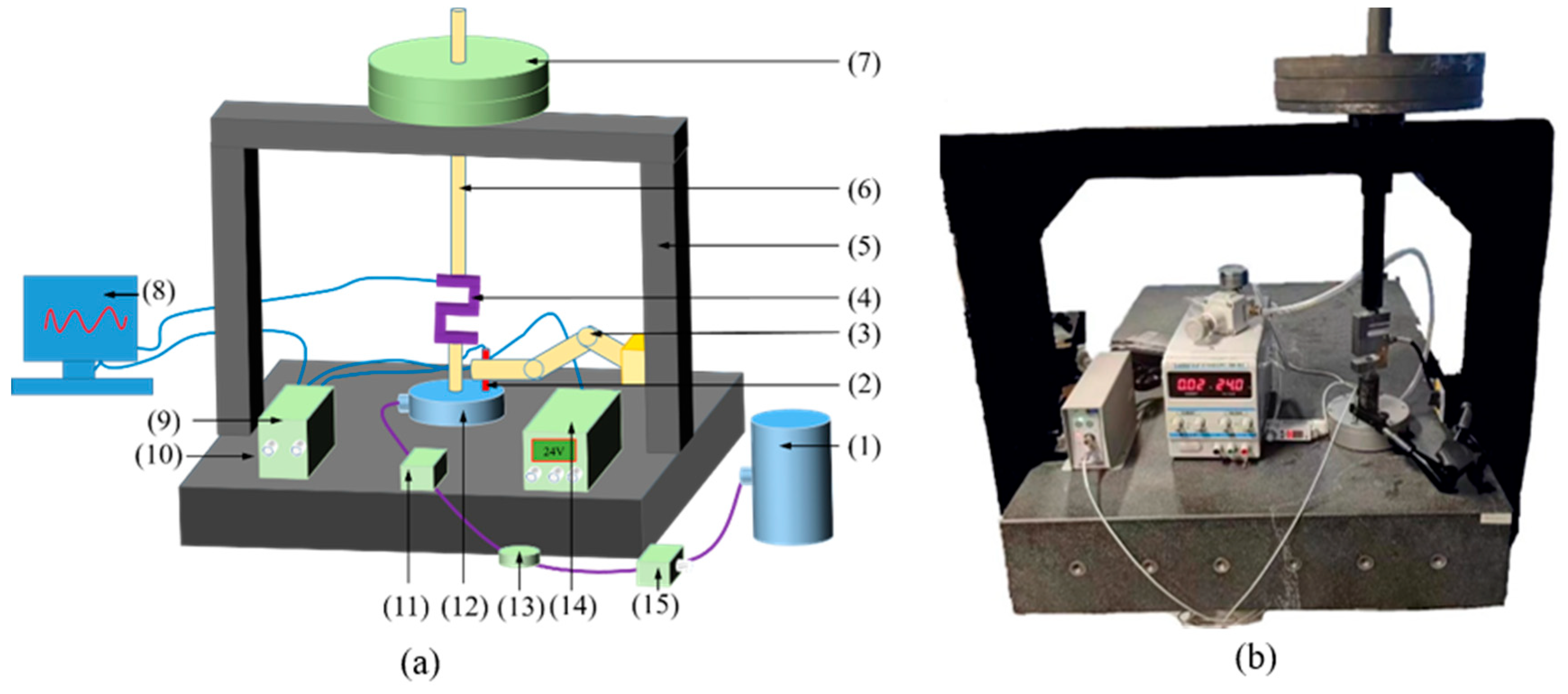
According to the simulation results, the optimal structural parameters of the bearing are obtained, and the bearing is manufactured according to the simulation parameters. It is necessary to test the static characteristics of bearings in atmospheric pressure and a vacuum environment to verify the accuracy of simulation results. The experimental apparatus for the static characteristics of the bearing in an atmospheric pressure environment is shown in Figure 5, consisting mainly of an air pump (1), LION PRECISION CPL592 non-contact capacitive displacement sensor is sourced from Lion, Dayton, OH, USA, (2), table stand (3), NS-WL1 force sensor is sourced from Tianmu, Shanghai, China (4), bracket (5), linear guide rod (6), weights (7), computer (8), data acquisition processing system (9), granite platform (10), SMC PFM711 flow meter is sourced from Gantuo, Shanghai, China (11), test bearing (12), pressure gauge (13), power supply (14), valve (15), etc. The entire test apparatus is leveled and placed on a vibration isolation platform.

Figure 5.
Static characteristic test of atmospheric pressure: (a) schematic diagram; (b) test equipment.
The air generated by the air pump is filtered and then connected to the supply orifice of the bearing to be tested through the pressure regulating valve, pressure gauge, flow meter, and micro-orifice restrictor. The bearing is lifted by the micro-orifice restrictor, forming an air film between the bearing and the platform to provide the bearing with load capacity. During the experiment, the bearing load can be changed by adjusting the mass of the weights, and the magnitude of the load is measured by a force sensor. The table frame is fixed on the column and clamps a non-contact capacitive displacement sensor. By measuring the displacement changes between the sensor and the bearing, the variation in the air film gap can be obtained. The measurement data are then transmitted to the computer to obtain the curve of the load capacity with the change in the air film thickness. The mass flow of the bearing is directly measured by the flow meter.
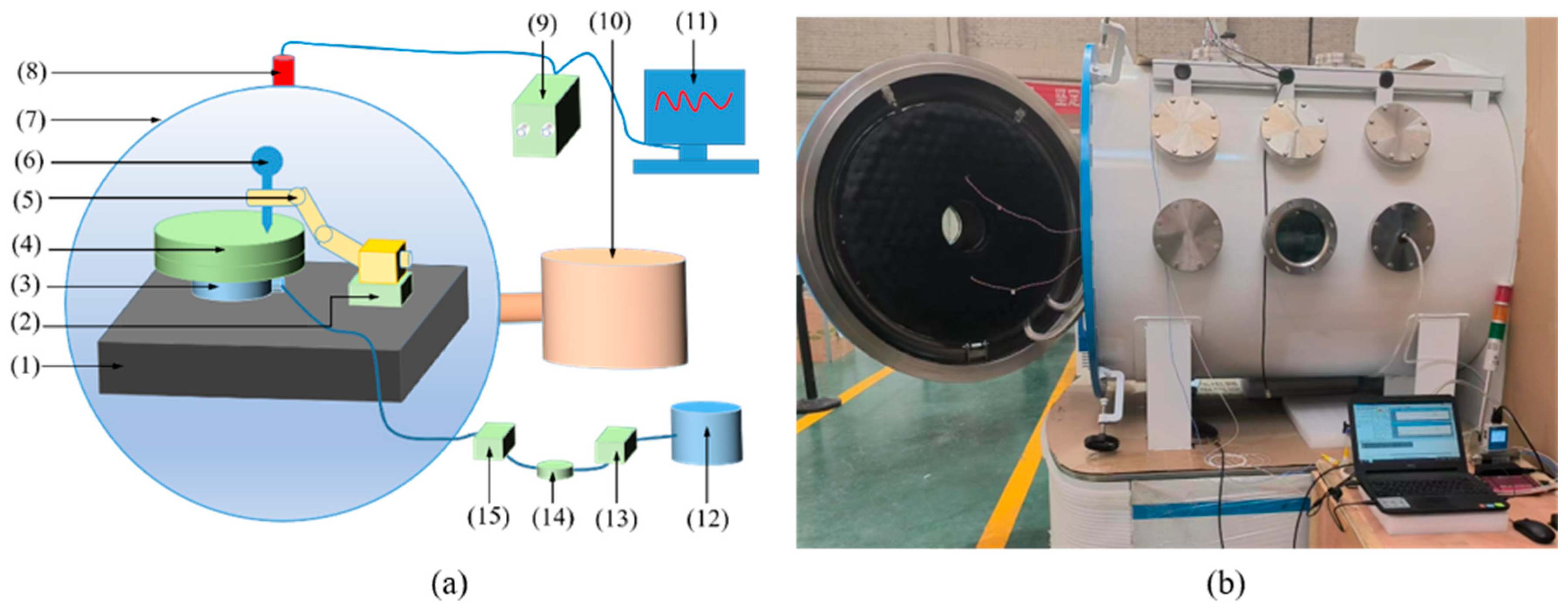
To test the static characteristics of aerostatic bearings under different air supply pressures and loads in a vacuum environment, a test platform was constructed, as shown in Figure 6. The test platform mainly consists of a measuring platform (1), a cushion block (2), a bearing to be tested (3), a weight (4), a gauge frame (5), a dial gauge (6), a vacuum tank (7), a ZJ51-T resistance gauge is sourced from Rui Bao Technology, Chengdu, China (8), a data acquisition and processing system (9), a vacuum pump (10), a computer (11), an air pump (12), a valve (13), a pressure gauge (14), and a flow meter (15).
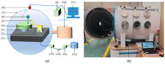
Figure 6.
Static characteristics test of different environmental pressures: (a) schematic diagram; (b) test equipment.
The bearings are placed into a vacuum chamber, where the internal pressure is adjusted by extracting the air with a vacuum pump. The pressure inside the chamber is monitored by a resistance gauge, which feeds the values back to the computer. The test bearings are placed on a measuring platform, and the load capacity is adjusted by varying the mass of the weights. A dial gauge is used to measure the changes in the air film thickness of the bearings, while the mass flow is measured in real time using a flow meter. During the experiment, the working environment of the bearings is controlled by adjusting the air supply pressure and the vacuum level of the vacuum chamber.
3.2. Experimental Methods
3.2.1. Experimental Conditions
Different working conditions are achieved by changing the external environmental pressure and air supply pressure. The setting of working conditions is shown in Table 1. In order to study the influence of vacuum degree on bearing performance, according to the experimental conditions and the suction rate of the vacuum tank, environmental pressures are set at 40,000 Pa, 37,000 Pa, 3500 Pa, 2800 Pa, 2500 Pa, 2300 Pa, 1600 Pa, 1100 Pa, 890 Pa. To ensure the accuracy of experimental data, multiple operating conditions are set to explore the performance of bearings. Air supply pressures are set at 0.1 MPa, 0.2 MPa, 0.3 MPa, 0.4 MPa, 0.5 MPa, and 0.6 MPa according to the pressure provided by the pump source.

Table 1.
Test conditions.
3.2.2. Variables of Experimental Measurement
Bearing capacity and mass flow are the variables measured in atmospheric and vacuum environments. In atmospheric conditions, the weight of the weight is changed; the change in bearing displacement is measured by a capacitance sensor; the change in air film thickness is obtained, and the mass flow is measured by the flow meter. Under different environmental pressures, the weight of the weight is changed; the change in bearing displacement is measured by the dial meter, and the mass flow is also measured by the flowmeter.
Considering the experimental error, three measuring points were taken for each working condition to measure the change in the air film thickness of the bearing, and the loading process and unloading were respectively measured and repeated three times. The average value of the obtained results is taken as the final experimental result, and finally, the experiment to obtain the influence of various parameters on bearing performance is conducted.
4. Results and Discussion
In addition to design variables, parameters set by simulation are shown in Table 2.
Table 2.
Setting of simulation parameters.
4.1. Influence of Geometric Parameters on Bearing Performance
4.1.1. Influence of Number of Orifices on Bearing Performance
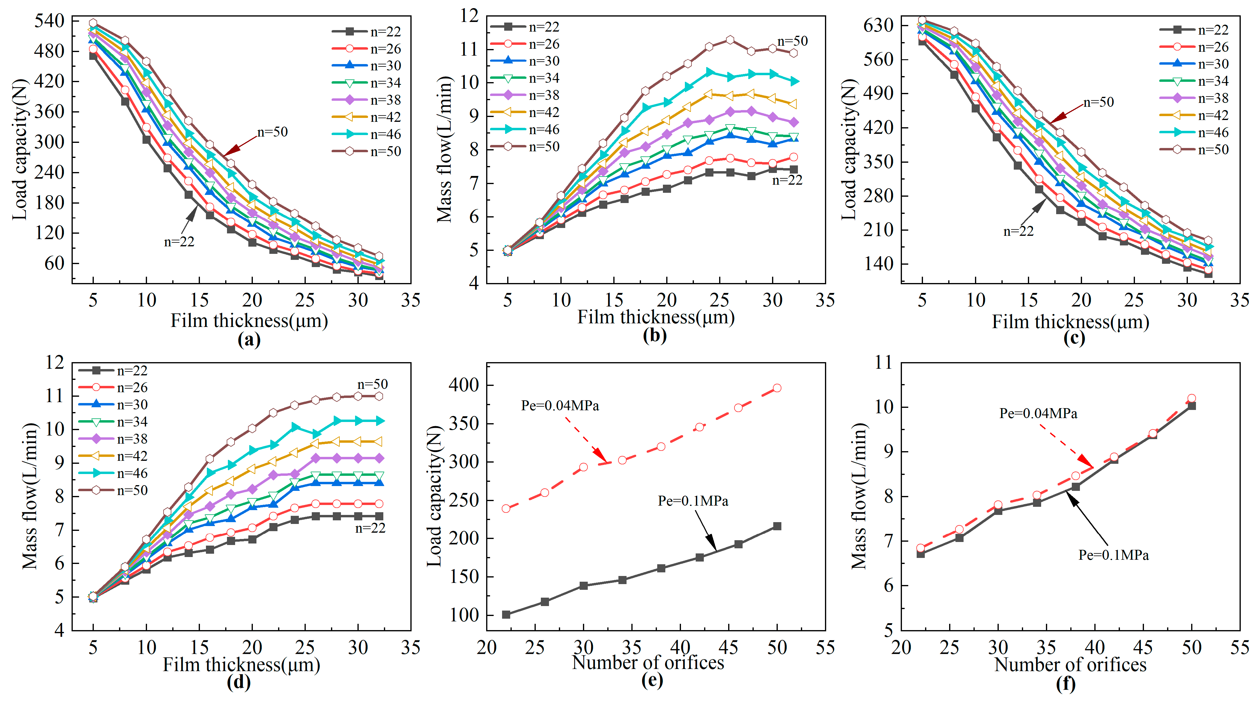
Figure 7 shows the variation in bearing capacity and mass flow with air film thickness and a number of orifices under normal pressure and 4000 Pa. In a vacuum environment, it can be observed from Figure 7c,e that the bearing load capacity decreases gradually with increasing air film thickness and increases with an increase in the number of orifices. When the number of orifices is 22, the bearing capacity is the smallest, and when the number of orifices is 50, the bearing capacity is the highest. According to Figure 7d, it can be seen that the mass flow of the air bearing increases with the increase in the air film thickness. When the air film thickness is 25 μm, the mass flow changes very slowly with the air film thickness. Therefore, when the air film thickness is large, the number of orifices has a more significant effect on the bearing mass flow, but when the air film thickness is between 10 μm and 20 μm, the number of orifices has a more significant effect on the bearing capacity. According to Figure 7f, it can be seen that the mass flow of the air bearing gradually increases with an increase in the number of orifices.
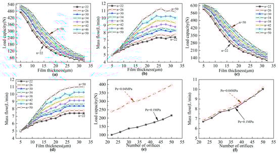
Figure 7.
Influence of air film thickness and number of orifices on bearing performance under different environmental pressures: (a) influence of air film thickness and orifice number on bearing capacity under atmospheric pressure; (b) influence of air film thickness and orifice number on mass flow under atmospheric pressure; (c) influence of 4000 Pa environmental air film thickness and the number of orifices on the bearing capacity; (d) influence of air film thickness and orifice number in 4000 Pa environment on mass flow; (e) influence of the number of orifices under different environmental pressure on the bearing capacity when the air film thickness is 20 μm; (f) influence of the number of orifices under different ambient pressure on the mass flow when the air film thickness is 20 μm.
In atmospheric pressure conditions, it can be deduced from Figure 7a,b,e,f that while the load capacity and mass flow of the bearing follow a similar trend as the thickness of the air film and the number of orifices in the vacuum environment, the bearing load capacity decreases by about 150 N, and the mass flow decreases by about 0.2 L/min compared with the vacuum environment. The reason for this is as follows: at an ambient pressure of 4000 Pa, the outlet pressure of the bearing is lower, resulting in a greater difference between the internal and external pressures of the bearing and a stronger load capacity. As the outlet pressure of the bearing decreases, the outlet flow rate is higher than atmospheric pressure, so the mass flow is also higher than atmospheric pressure.
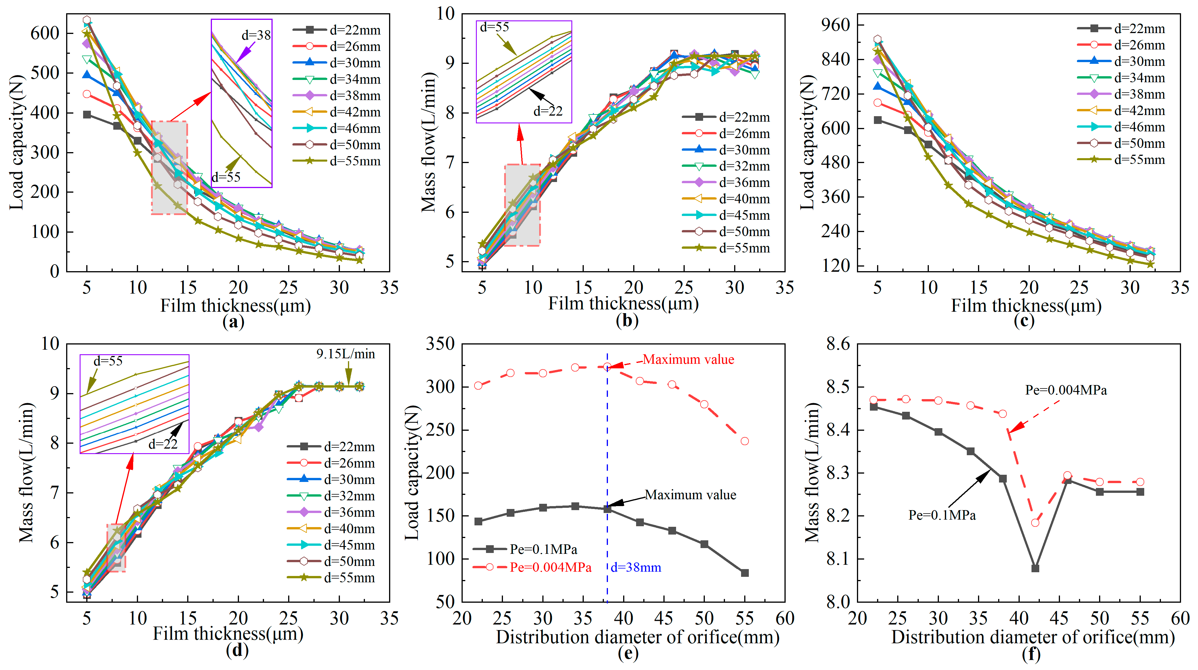
4.1.2. Influence of Distribution Diameter of Orifice on Bearing Performance
Figure 8 shows the variations in bearing load capacity and mass flow of the bearing with changes in air film thickness and orifice distribution diameter at atmospheric pressure and 4000 Pa.
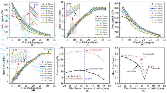
Figure 8.
Influence of air film thickness and orifice distribution diameter on bearing performance under different environmental pressures: (a) influence of air film thickness and orifice distribution diameter on bearing capacity under atmospheric pressure; (b) influence of air film thickness and orifice distribution diameter on mass flow under atmospheric pressure; (c) influence of air film thickness and orifice distribution diameter on bearing capacity in 4000 Pa environment; (d) influence of air film thickness and orifice distribution diameter on mass flow in 4000 Pa environment; (e) influence of the distribution diameter of orifice under different ambient pressure on the bearing capacity when the air film thickness is 20 μm; (f) influence of different ambient pressure distribution diameters on mass flow when the air film thickness is 20 μm.
In a vacuum environment, it can be observed from Figure 8c,e that with the increase in the orifice distribution diameter, the load capacity of the bearing first increases and then decreases. When the orifice distribution diameter is 38 mm, the bearing has the maximum load capacity, while at 55 mm, it has the minimum load capacity. The reason behind this phenomenon lies in the formation of a stable high-pressure zone as the air flows from the orifice toward the center of the bearing. When the orifice is closer to the center position, the proportion of the intermediate high-pressure zone is relatively small, resulting in a lower bearing load capacity. As the orifice distribution diameter gradually increases, the proportion of the intermediate high-pressure zone also increases, leading to an enhancement in the bearing load capacity. However, as the orifice distribution diameter continues to increase, the orifice approaches the bearing outlet, causing the air to rapidly overflow from the outlet, thereby reducing the bearing load capacity. According to Figure 8d, it is evident that when the air film thickness is less than 25 μm, the mass flow of the bearing increases slowly with the increase in orifice position. When the air film thickness exceeds 25 μm, the mass flow of the bearing is 9.15 L/min and remains constant as the orifice distribution diameter no longer changes.
In the atmospheric environment, it can be inferred from Figure 8a,b,e,f that the overall trends of load capacity and mass flow follow a similar pattern to that of the vacuum environment. However, the load capacity value decreases by approximately 160 N compared to the vacuum environment, while the maximum mass flow decreases by around 0.2 L/min. Based on the analysis above, when the orifice distribution diameter is 38 mm, the bearing exhibits a higher load capacity.
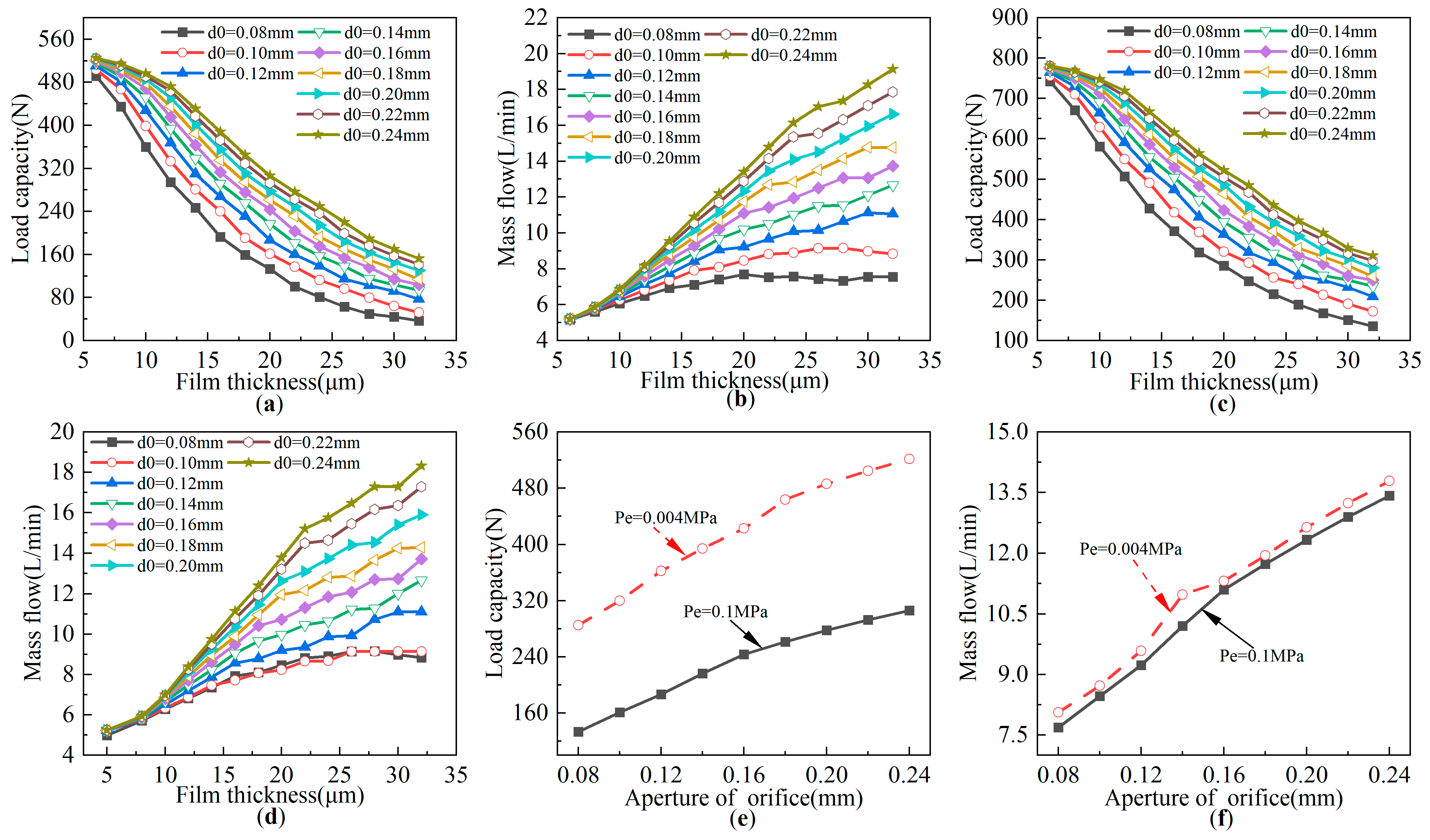
4.1.3. Influence of Orifice Aperture on Bearing Performance
Figure 9 shows the variation in bearing capacity and mass flow with air film thickness and orifice aperture under atmospheric pressure and 4000 Pa.
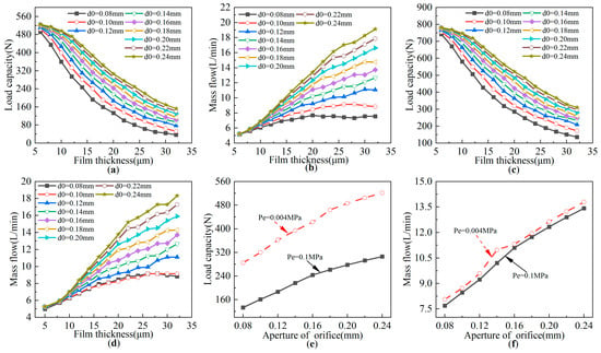
Figure 9.
Influence of air film thickness and orifice aperture on bearing performance under different environmental pressures: (a) influence of air film thickness and orifice aperture on load capacity in atmospheric pressure conditions; (b) influence of air film thickness and orifice aperture on mass flow in atmospheric pressure conditions; (c) influence of air film thickness and orifice aperture on load capacity under 4000 Pa environmental pressure; (d) influence of air film thickness and orifice aperture on mass flow under 4000 Pa environmental pressure; (e) influence of orifice aperture on load capacity under varying environmental pressures with an air film thickness of 20 μm; (f) influence of orifice aperture on mass flow under varying environmental pressures with an air film thickness of 20 μm.
According to Figure 9, it can be seen that at atmospheric and environmental pressures of 4000 Pa, as the orifice aperture increases, the bearing capacity and mass flow gradually increase. Moreover, the bearing capacity in a vacuum is 200 N higher than atmospheric pressure, and the mass flow is 0.1–0.2 L/min higher than atmospheric pressure. When the air film thickness is between 10 μm and 20 μm, the bearing’s load capacity uniformly changes with the orifice aperture, while the mass flow of the bearing increases slowly. When the air film thickness exceeds 20 μm, the gradient of load capacity change remains consistent with before, but the mass flow increases rapidly. The reason is that the larger the orifice aperture, the larger the throttling area, and when the air film thickness is large, the outlet pressure of the bearing is very small, resulting in a higher flow rate, ultimately leading to a rapid increase in the mass flow of the bearing. When the load is constant, the air film thickness of the bearing in a vacuum is higher than that under atmospheric pressure. Therefore, the air film thickness of the bearing should not be too high. Based on the influence of the number and diameter of the orifices on the bearing performance, the air film thickness should be selected as 20 μm.
4.2. Influence of Environmental Conditions on Bearing Performance
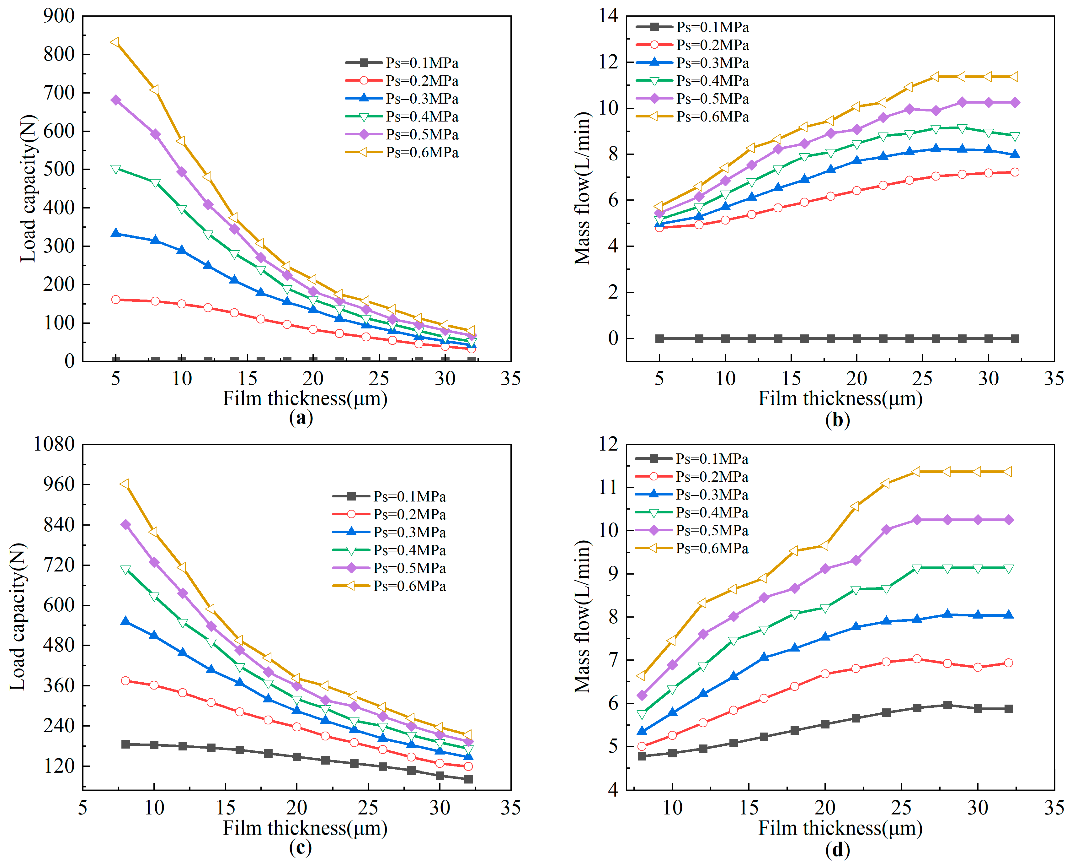
4.2.1. Influence of Air Supply Pressure on Bearing Performance
Figure 10 shows the influence of air supply pressure on the performance of bearings under atmospheric pressure and an ambient pressure of 4000 Pa.
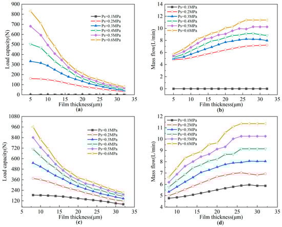
Figure 10.
Influence of air supply pressure on bearing performance under different environmental pressures: (a) influence of atmospheric air supply pressure on the bearing capacity; (b) influence of atmospheric air supply pressure on mass flow; (c) influence of 4000 Pa ambient air supply pressure on the bearing capacity; (d) influence of 4000 Pa ambient air supply pressure on mass flow.
According to Figure 10, it can be seen that at atmospheric and environmental pressures of 4000 Pa, the bearing capacity and mass flow of the bearing increase with the increase in air supply pressure. When the air supply pressure is 0.2 MPa, the bearing capacity increases slowly with the decrease in air film thickness, and the mass flow also increases slowly. When the air supply pressure is increased to 0.6 MPa, the bearing capacity increases rapidly with the decrease in film thickness, and the mass flow increases rapidly. When the environmental pressure is 4000 Pa, the bearing capacity is increased by about 20% compared with atmospheric pressure, and the mass flow is about 1.05 times atmospheric. In the vacuum environment, the floating amount increases compared with the normal pressure. To mitigate the self-excited vibration of the bearings and enhance their stability, the air supply pressure of 0.4 MPa is recommended based on Figure 10.
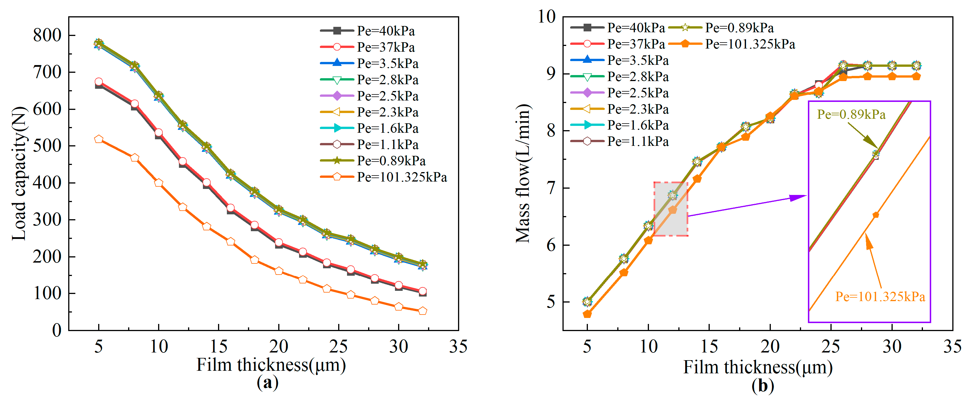
4.2.2. Influence of Environmental Pressure on Bearing Performance
Figure 11 shows the variation in bearing capacity and mass flow with air film thickness under different environmental pressures. According to Figure 11a, bearing capacity gradually increases with the reduction in environmental pressure. When the environmental pressure is 37 kPa to 40 kPa, the bearing capacity increases by about 30% compared with atmospheric pressure; when the environmental pressure is reduced below 3.5 kPa, the bearing capacity is increased by about 50% compared to the atmospheric pressure environment. The bearing capacity increases very slowly by continuing to reduce the environmental pressure. According to Figure 11b, it can be seen that the mass flow of the bearing in vacuum increases by about 5% compared with the atmospheric pressure environment, but the mass flow increases very slowly with the increase in vacuum degree. Therefore, when the vacuum degree is about 3.5 kPa, the bearing capacity and mass flow reach the best parameters.
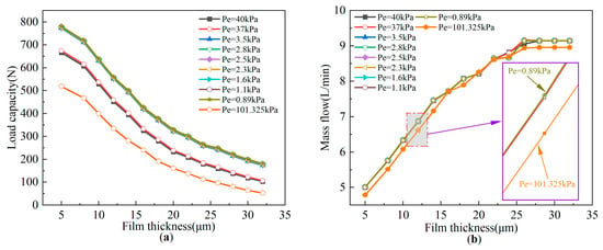
Figure 11.
Influence of different environmental pressures on bearing performance: (a) influence of different environmental pressures on the bearing capacity; (b) influence of different environmental pressures on mass flow.
4.3. Pareto Frontier Optimal Solution
Transfer functions such as trainlm, trainbr, trainscg, and traingdx are used for fitting . The determination coefficients obtained according to Equation (12) are 0.9621, 0.9997, 0.9977, and 0.9650, respectively. Therefore, trainbr is selected to train the data to obtain .
When the ambient pressure is 3500 Pa, the air supply pressure is 0.4 MPa, and the air film thickness is 20 μm; the optimal solution of the Pareto front of the objective function is shown in Figure 12. According to Figure 12, a total of 29 groups of optimal solutions were obtained by using the optimization algorithm, and the G value was the 28th solution. In this case, the distribution diameter of the orifice corresponding to the 28th solution is 38.83 mm; the number of orifices is 36, and the aperture of the orifice is 0.1 mm. At this time, the corresponding bearing capacity in the vacuum environment is 460.644 N, and the mass flow is 11.816 L/min. According to this parameter, the static test of the bearing is carried out under different air supply pressure and environmental pressure.
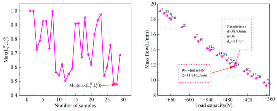
Figure 12.
Pareto frontier optimal solution.
In order to verify the accuracy of the NSGA-II multi-objective optimization algorithm, particle swarm optimization algorithm, simulated annealing algorithm, and Tabu search algorithm were used to obtain bearing capacity and mass flow. The results are shown in Table 3. It can be seen from Table 3 that compared with other algorithms, the ratio of carrying capacity to mass flow obtained by the NSGA-II algorithm is the largest, and the solution is optimal under this algorithm.
Table 3.
Algorithm comparison.
4.4. Comparison between Simulation and Experiment
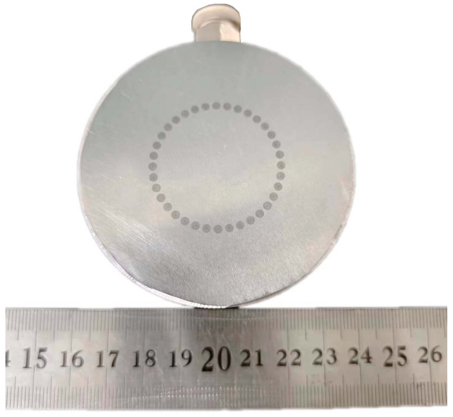
The bearing material is S136 stainless steel made in Tianjin, China. In the case of high load and small mass flow, the optimized bearing parameters are shown in Table 4. The physical picture of the bearing is shown in Figure 13.
Table 4.
Bearing parameters.

Figure 13.
Bearing picture.
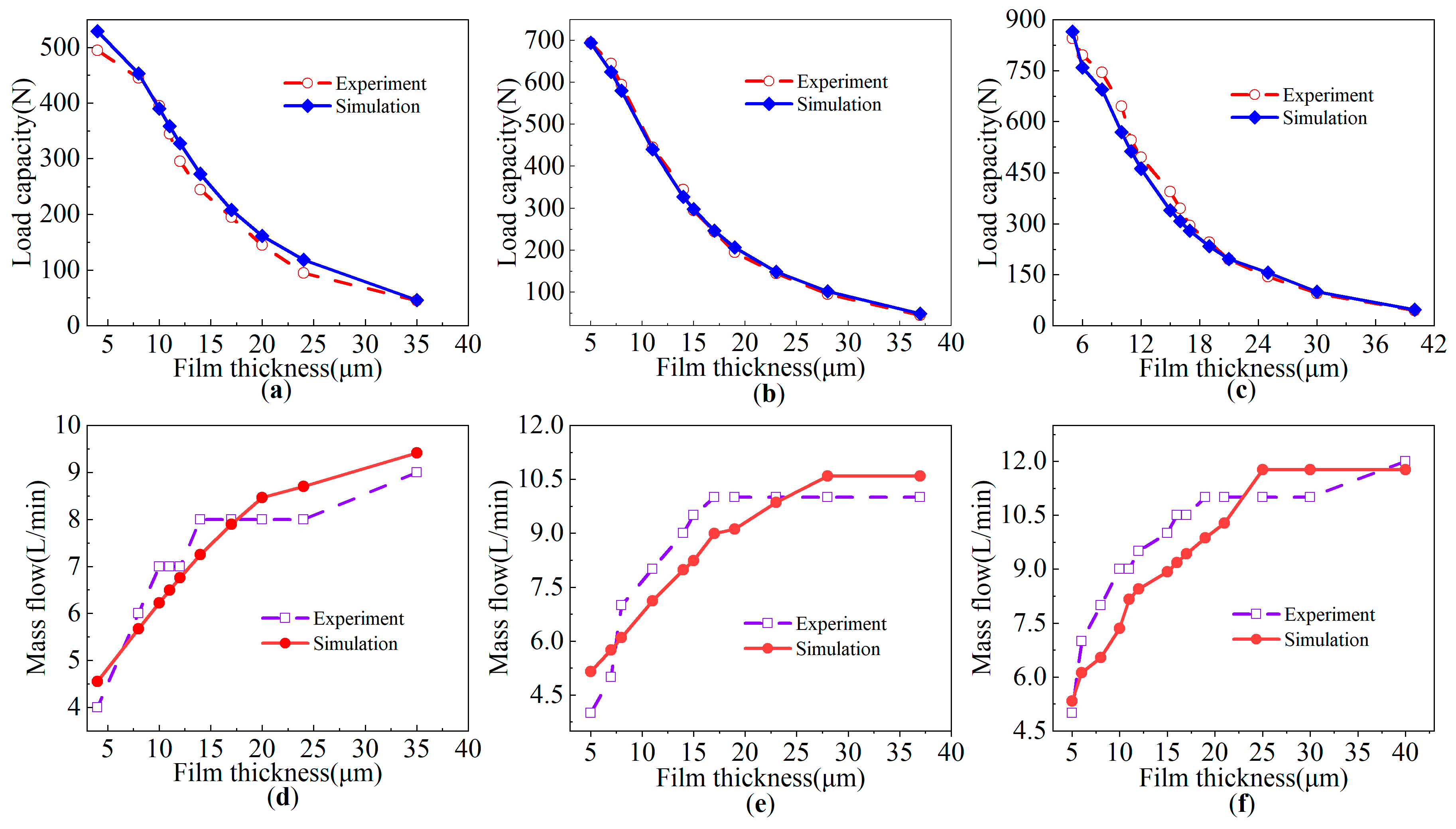
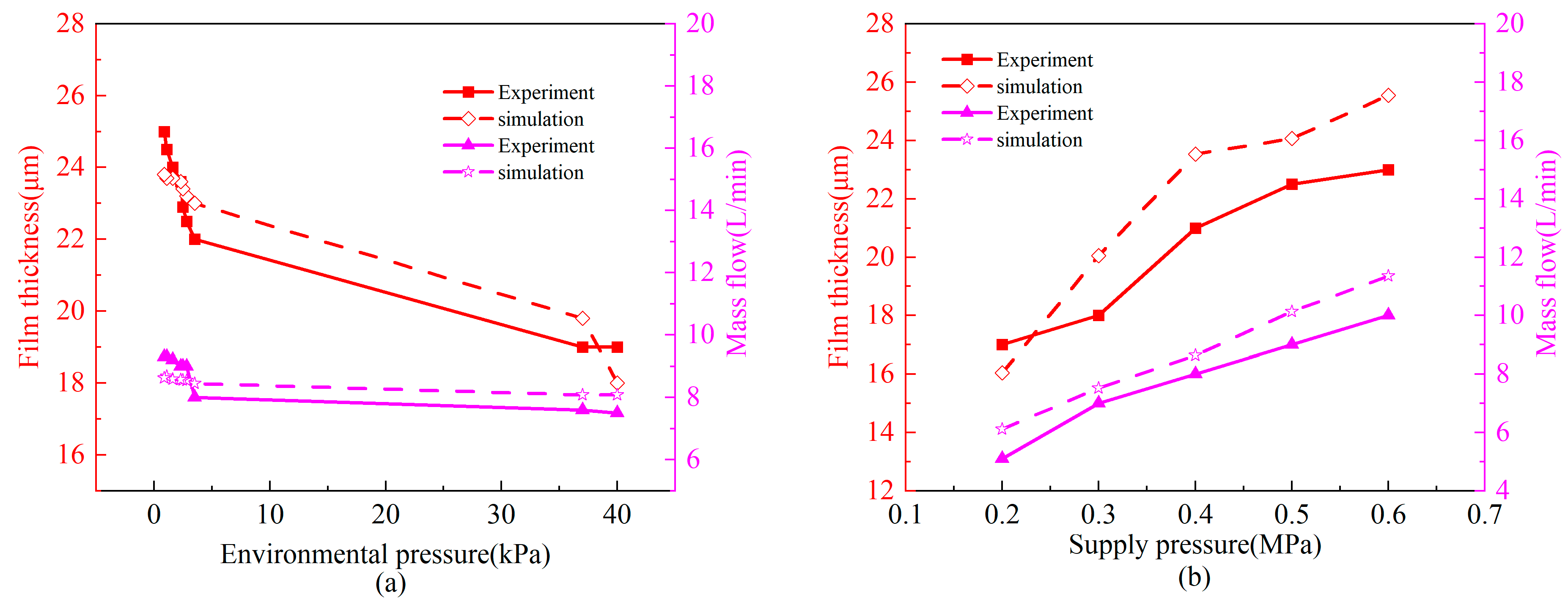
When the ambient pressure is 0.1 MPa, and the air supply pressure is 0.4 MPa, 0.5 MPa, and 0.6 MPa, respectively, the bearing capacity and mass flow obtained by simulation and test are shown in Figure 14. According to Figure 14, under different air supply pressures, bearing capacity decreases with the increase in air film thickness, and mass flow increases with the increase in air film thickness. The load capacity and mass flow obtained by simulation are in good agreement with the experimental values. To further verify the correctness of the simulation, the influence of different environmental pressure and supply pressures on the bearing air film thickness when the bearing load is 280 N was tested, and the results are shown in Figure 15.
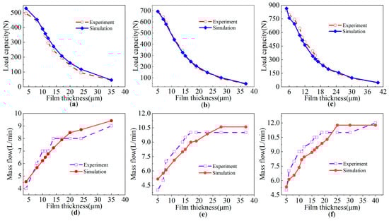
Figure 14.
Comparison of simulation and experiment in atmospheric pressure environment: (a) comparison of bearing capacity when Ps = 0.4 MPa; (b) comparison of bearing capacity when Ps = 0.5 MPa; (c) comparison of bearing capacity when Ps = 0.6 MPa; (d) mass flow comparison when Ps = 0.4 MPa; (e) mass flow comparison when Ps = 0.5 MPa; (f) mass flow comparison when Ps = 0.6 MPa.
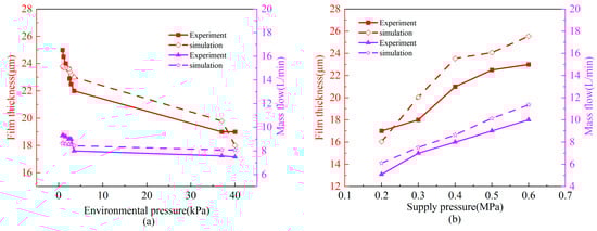
Figure 15.
Comparison of simulation and experiment under different environmental pressures and different air supply pressures: (a) comparison of simulation and experiment of different environmental pressures; (b) comparison of simulation and experiment of different air supply pressures.
According to Figure 15a, the air film thickness and mass flow gradually increase with the decrease in environmental pressure. The reason is that the bearing outlet flow rate gradually increases with the reduction in pressure, so when the load is constant, the air film thickness is higher, and the flow rate is larger. According to Figure 15b, when the load is constant, the air film thickness and mass flow increase with the increase in air supply pressure. The maximum error of the whole test is about 10%. The main reasons for the difference between the theoretical value and the test value are as follows: First, the flatness error of the bearing surface and the inclination of the bearing during measurement are not considered in the simulation. Second, the external environment, such as noise and equipment vibration, will cause fluctuations in the thickness of the air film. In addition, according to the previous analysis, the orifice aperture has a great impact on the bearing performance. Because the orifice aperture is small and difficult to process, it will produce errors with the simulated theoretical value. Considering the influence of processing and assembly errors, we have taken a safety factor of 1.5 times under rated load conditions, so it still meets the requirements for use under this error.
5. Conclusions
In this paper, the influence of different parameters and external environments on the bearing capacity and mass flow of air bearings applied in a vacuum environment were analyzed by combining numerical simulation and experimental verification, and the bearing structure was optimized. The following conclusions were reached:
- 1.
- In the vacuum environment, because the outlet pressure of the bearing is lower than that of the atmospheric pressure, the pressure difference between the inside and outside of the bearing increases, and the outlet flow rate increases, resulting in the bearing capacity and flow rate being increased compared with the atmospheric pressure environment and gradually increasing with the decrease in vacuum degree;
- 2.
- With the optimization goals of maximum load capacity and minimum mass flow of bearings in the vacuum, the objective function was fitted using a BP neural network and combined with the NSGA-II multi-objective optimization algorithm to optimize the bearing parameters. When the bearing’s aperture of the orifice is 0.1 mm, the number of orifices is 36, and the distribution diameter of the orifice is 38.83 mm, the bearing has a maximum load capacity of 460.644 N and a minimum mass flow rate of 11.816 L/min;
- 3.
- Experiments are carried out on the optimized bearing parameters in atmospheric pressure and vacuum environments. The maximum error between the experimental and theoretical values is 10%, which verified the correctness and feasibility of the simulation and provided a theoretical and experimental method for the design of the aerostatic thrust bearing in a vacuum;
- 4.
- When designing bearings for application in a vacuum environment, the optimization and experimental methods proposed in this paper can quickly design ideal parameters, greatly improving the efficiency of design. This is of great significance for the design, manufacturing, and maintenance of bearings;
- 5.
- Although the optimization method of bearing parameters presented in this paper is carried out under specific fields, materials, and experimental conditions, the analysis and calculation methods presented in this paper are still of popularization significance for other fields, materials, and experimental conditions. In future studies, we will try to obtain the output values for how to use numerical methods in other experimental conditions.
Author Contributions
Conceptualization, G.F. and Y.L. (Youhua Li); methodology, G.F. and H.Y.; software, J.X. and G.F.; validation, Z.L. and M.Z.; formal analysis, Y.L. (Yuehua Li) and H.L.; investigation, H.L. and W.H.; data curation, G.F. and W.H.; writing—original draft preparation, G.F. and H.Y.; writing—review and editing, Z.L. and L.Z.; visualization, H.Y. and G.Z.; funding acquisition, H.Y. and M.Z. All authors have read and agreed to the published version of the manuscript.
Funding
This research was funded by the National Nature Science Foundation of China, grant number 51875586; the Tianjin Natural Science Foundation grant number 22JCZDJC00910.
Data Availability Statement
The original contributions presented in the study are included in the article material, further inquiries can be directed to the authors.
Conflicts of Interest
The authors declare no conflicts of interest.
References
- Wapman, J.D.; Sternberg, D.C.; Lo, K.; Wang, M.; Jones-Wilson, L.; Mohan, S. Jet Propulsion Laboratory Small Satellite Dynamics Testbed Planar Air-Bearing Propulsion System Characterization. J. Spacecr. Rockets 2021, 58, 954–971. [Google Scholar] [CrossRef]
- Miyatake, M.; Yoshimoto, S. Numerical investigation of static and dynamic characteristics of aerostatic thrust bearings with small feed holes. Tribol. Int. 2010, 43, 1353–1359. [Google Scholar] [CrossRef]
- Gao, S.; Cheng, K.; Chen, S.; Ding, H.; Fu, H. Computational design and analysis of aerostatic journal bearings with application to ultra-high speed spindles. Proc. Inst. Mech. Eng. Part C 2017, 231, 1205–1220. [Google Scholar] [CrossRef]
- Chakraborty, B.; Bhattacharjee, B.; Chakraborti, P.; Biswas, N. Evaluation of the performance characteristics of aerostatic bearing with porous alumina (Al2O3) membrane using theoretical and experimental methods. Proc. Inst. Mech. Eng. Part J 2024, 13506501241245760. [Google Scholar] [CrossRef]
- Khim, G.; Park, C.H.; Lee, H.; Kim, S.W. Analysis of additional leakage resulting from the feeding motion of a vacuum-compatible air bearing stage. Vacuum 2006, 81, 466–474. [Google Scholar] [CrossRef]
- Fukui, S.; Kaneko, R. Experimental Investigation of Externally Pressurized Bearings Under High Knudsen Number Conditions. J. Tribol. 1988, 110, 144–147. [Google Scholar] [CrossRef]
- Trost, D. Design and analysis of hydrostatic gas bearings for vacuum applications. In Proceedings of the ASPE Spring Topical Meeting on Challenges at the Intersection of Precision Engineering and Vacuum Technology, Orlando, FL, USA, 2 April 2006. [Google Scholar]
- Schenk, C.; Buschmann, S.; Risse, S.; Eberhardt, R.; Tünnermann, A. Comparison between flat aerostatic gas-bearing pads with orifice and porous feedings at high-vacuum conditions. Precis. Eng. 2008, 32, 319–328. [Google Scholar] [CrossRef]
- Gans, R. Lubrication theory at arbitrary Knudsen number. J. Tribol. 1985, 107, 431–433. [Google Scholar] [CrossRef]
- Chan, C.-W. Modified Particle Swarm Optimization Algorithm for Multi-Objective Optimization Design of Hybrid Journal Bearings. J. Tribol. 2015, 137, 021101. [Google Scholar] [CrossRef]
- Wang, N.; Chang, Y.Z. Application of the Genetic Algorithm to the Multi-Objective Optimization of Air Bearings. Tribol. Lett. 2004, 17, 119–128. [Google Scholar] [CrossRef]
- Wang, N.; Cha, K.-C. Multi-objective optimization of air bearings using hypercube-dividing method. Tribol. Int. 2010, 43, 1631–1638. [Google Scholar] [CrossRef]
- Yifei, L.; Yihui, Y.; Hong, Y.; Xinen, L.; Jun, M.; Hailong, C. Modeling for optimization of circular flat pad aerostatic bearing with a single central orifice-type restrictor based on CFD simulation. Tribol. Int. 2017, 109, 206–216. [Google Scholar] [CrossRef]
- Wang, N.; Chen, H.-Y. A two-stage multiobjective optimization algorithm for porous air bearing design. Tribol. Int. 2016, 93, 355–363. [Google Scholar] [CrossRef]
- Zhang, T.; Chen, L.; Wang, J. Multi-objective optimization of elliptical tube fin heat exchangers based on neural networks and genetic algorithm. Energy 2023, 269, 126729. [Google Scholar] [CrossRef]
- Wang, G.; Li, W.; Liu, G.; Feng, K. A novel optimization design method for obtaining high-performance micro-hole aerostatic bearings with experimental validation. Tribol. Int. 2023, 185, 108542. [Google Scholar] [CrossRef]
- Chang, L.; Tenghui, J.; Xing, H.; Xiansheng, J. Study on parameter optimization of laser cladding Fe60 based on GA-BP neural network. J. Adhes. Sci. Technol. 2023, 37, 2556–2586. [Google Scholar]
- Gao, F.; Zheng, Y.; Li, Y.; Li, W. A back propagation neural network-based adaptive sampling strategy for uncertainty surfaces. Trans. Inst. Meas. Control. 2024, 46, 1012–1023. [Google Scholar] [CrossRef]
- Ding, C.; Ding, Y.; Yuan, Z.; Li, J. Structural Optimization Design of Electromagnetic Repulsion Mechanism Based on BP Neural Network and NSGA–II. IEEJ Trans. Electr. Electron. Eng. 2023, 18, 1914–1922. [Google Scholar]
- Guofang, L.; Xing, L.; Meng, L.; Tong, N.; Shaopei, W.; Wangcai, D. Multi-objective optimisation of high-speed rail profile with small radius curve based on NSGA-II Algorithm. Veh. Syst. Dyn. 2023, 61, 3111–3135. [Google Scholar]
- Kim, I.Y.; de Weck, O.L. Adaptive weighted-sum method for bi-objective optimization: Pareto front generation. Struct. Multidiscip. Optim. 2005, 29, 149–158. [Google Scholar] [CrossRef]
- Xu, X.F.; Xu, S.; Zhou, T. An Improved Spectral Clustering Algorithm Using Minimum Maximum Principle. Appl. Mech. Mater. 2012, 1810, 1881–1884. [Google Scholar] [CrossRef]

Disclaimer/Publisher’s Note: The statements, opinions and data contained in all publications are solely those of the individual author(s) and contributor(s) and not of MDPI and/or the editor(s). MDPI and/or the editor(s) disclaim responsibility for any injury to people or property resulting from any ideas, methods, instructions or products referred to in the content. |
© 2024 by the authors. Licensee MDPI, Basel, Switzerland. This article is an open access article distributed under the terms and conditions of the Creative Commons Attribution (CC BY) license (https://creativecommons.org/licenses/by/4.0/).