A Graph-Data-Based Monitoring Method of Bearing Lubrication Using Multi-Sensor

Abstract

Super-precision bearing lubrication condition is essential for equipment’s overall performance. This paper investigates a monitoring method of bearing lubrication using multi-sensors based on graph data. An experiment was designed and carried out, establishing a dataset including vibration, temperature, and acoustic emission signals. Graph data were constructed based on a priori knowledge and a graph attention network was employed to conduct a study on monitoring bearing lubrication abnormalities and discuss the influence of a missing sensor on the monitoring. The results show that the designed experiments can effectively respond to the degradation process of bearing lubrication, and the graph data constructed based on a priori knowledge show a good effect in the anomaly monitoring process. In addition, the multi-sensor plays a significant role in monitoring bearing lubrication. This work will be highly beneficial for future monitoring methods of bearing lubrication status.

1. Introduction

Super-precision bearings are critical components in CNC machines, high-speed machining centers, and other advanced devices [1,2,3]. These bearings’ operational state directly impacts the equipment’s overall performance. Super-precision bearings typically operate under light load and high-speed conditions, resulting in low contact stress at the ball raceway. Consequently, spalling is rare in super-precision bearings. Instead, lubrication problems and related friction and wear have become the predominant failure modes. For instance, NSK statistics show that over 70% of bearing failures in the machine tool are due to surface damage caused by contamination and lubrication [4]. NTN has identified that the main failure modes of machine tool spindle bearings are surface roughening, micro-spalling, and burning due to wear [5]. Data on precision machine tool spindle bearing failures in China indicate that surface damage due to wear and lubrication burning account for up to 80% of failures [6]. Therefore, accurately monitoring the lubrication state of bearings is crucial for ensuring super-precision bearings’ safe and reliable operation.

Most research on bearing condition monitoring focuses on monitoring fatigue damage, fault location, and fault quantification using vibration caused by spalling. However, during the early stages of bearing lubrication failure, partial oil film breakdown or contamination can cause rough contact between the rolling elements and the inner and outer raceways, generating pulses and exciting the natural frequencies of the bearing components, thus producing high-frequency vibration signals [7]. High-bandwidth sensors can detect these high-frequency vibration signals. However, commonly used piezoelectric vibration accelerometers typically have a bandwidth of less than 30 kHz [8], while the frequencies associated with early lubrication state signals are usually above 30 kHz [9,10,11], which makes it challenging to detect early lubrication failures in bearings using vibration accelerometers. Therefore, traditional condition monitoring methods are not suitable for lubrication state monitoring.

Xu et al. [12] proposed a vibration-based bearing lubrication state identification scheme, using minimum entropy deconvolution to enhance random pulses and construct a spectral centroid feature to diagnose lubrication conditions. Miettinen et al. [13] conducted acoustic emission (AE) tests on grease-lubricated bearings using the “pulse counting method”, where pulses exceeding a specified voltage were counted. They found this method helpful for monitoring contamination levels in grease-lubricated bearings and predicting grease starvation levels. Yoshioka et al. [14] developed a combined vibration-AE sensor and applied it to bearing fatigue experiments. The results demonstrated that the AE sensor could detect bearing damage earlier than the vibration acceleration sensor. Benefiting from advances in modern computer technology, Fan et al. [15] conducted experimental research using AE technology on rolling bearings without lubricants and rolling bearings with contaminated grease. High-frequency sampling and data streaming techniques were applied to measure AE. The conditions of bearings without grease and those with contaminated grease could be clearly distinguished by processing the AE signals using frequency domain analysis. Krishnamoorthy et al. [16] studied the correlation between the AE signals generated during the friction between self-lubricating coatings and steel surfaces and found the root mean square (RMS) of the acoustic signal was correlated with the coefficient of friction generated during the tribo-pair interaction.

The studies mentioned above demonstrate that signals such as temperature, vibration, and AE can reflect the lubrication state. However, each signal has limitations due to the complexity of actual industrial environments. Temperature signals are easily influenced by ambient temperature, cooling conditions, and load; vibration signals may be confused with other bearing fault signals, and ambient noise can interfere with acoustic emission signals. Additionally, relying on a single indicator may overlook the complexity of the lubrication state, thus increasing the risk of misjudgment or missed diagnosis. Therefore, it is necessary to integrate multiple sensors and advanced analytical methods for monitoring and diagnosing bearing lubrication [17,18].

In recent years, the introduction of graph data analysis techniques has brought new possibilities for addressing the complexity of bearing fault diagnosis [17,19,20,21]. By representing the relationships between various monitoring variables as a graph, it is possible to better capture these complex coupling relationships. Therefore, with the aid of graph data analysis techniques, it is expected that the overall state of bearings can be better monitored, improving the accuracy and reliability of lubrication condition monitoring. Michael et al. [22] utilized mechanism analysis to simulate second-order structures of edge signals in data centers with graph data, efficiently locating link faults in data centers. Zhao et al. [23] proposed a multi-scale deep graph convolutional network based on multi-scale data fusion and multi-scale graph convolutional kernel fusion. They used a sliding window to segment collected vibration signals into a series of sub-signals for multi-scale signal processing and designed graph convolutions with multi-scale kernels to fuse global features, achieving intelligent monitoring of bearing systems. While the models above have made progress in considering system integrity and complex coupling relationships, they often face challenges due to a lack of sufficient prior knowledge, resulting in unknown or difficult-to-construct graph structures [24]. Additionally, traditional methods predominantly employ static graph data models, which cannot accurately describe the dynamic changes in bearing states, limiting model adaptability and predictive accuracy [25]. Moreover, super-precision bearings are known for their high reliability, making it extremely difficult to acquire failure datasets. The scarcity of failure datasets poses significant challenges for bearing state monitoring research.

This paper explores a graph-based bearing lubrication condition monitoring method with multi-sensors, including vibration, temperature, and AE. To solve the data scarcity problem, we first conducted experiments on the bearing lubrication failure process, obtaining vibration, temperature, and AE signals. Then, based on prior knowledge, these signals were processed to select time-frequency features closely related to lubrication conditions, and graph data describing the bearing lubrication state were constructed. Subsequently, a study on bearing lubrication condition monitoring based on GAN was conducted, and the impact of missing sensor signals on monitoring is discussed.

2. Experiment and Analysis

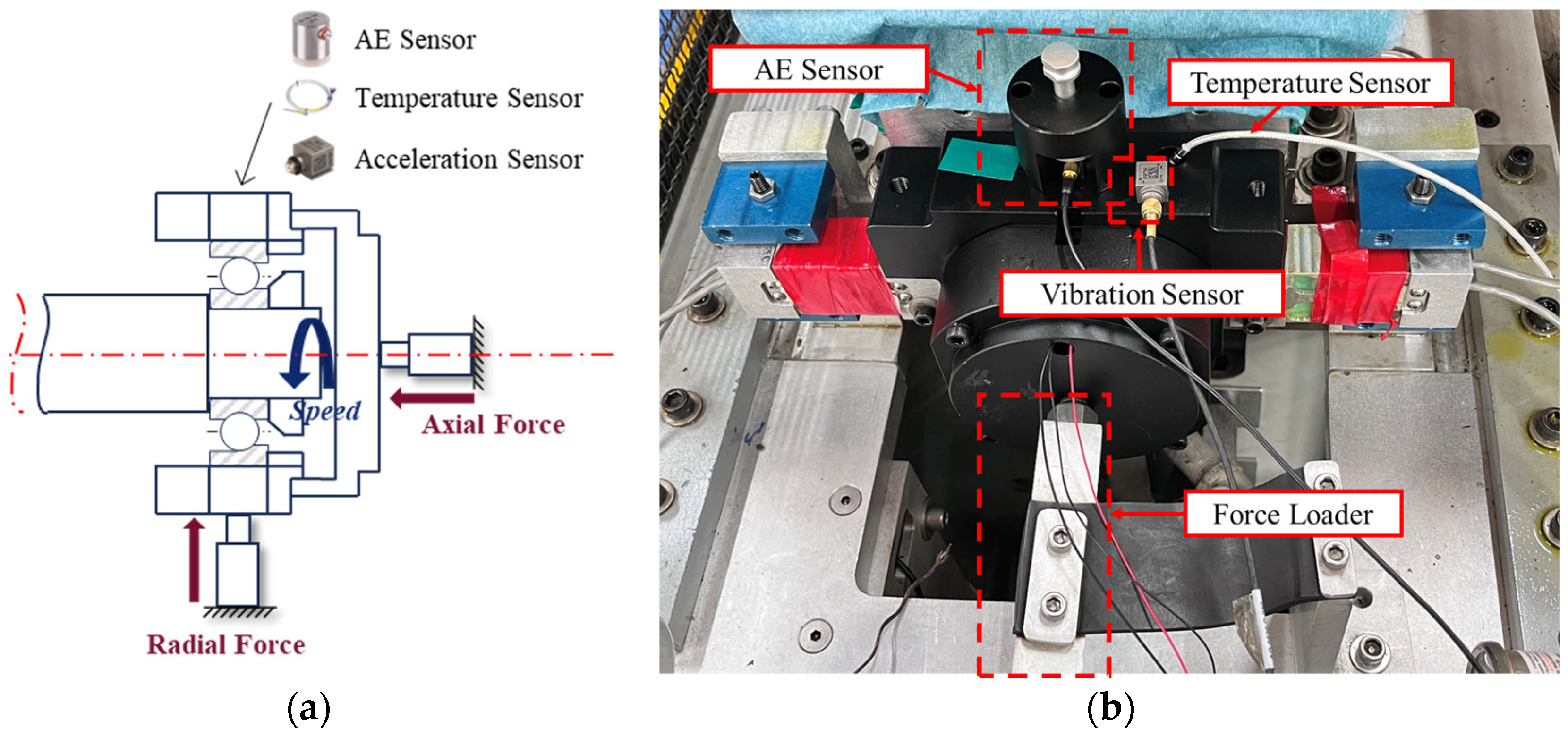
2.1. Experiment Description

The bearing lubrication failure simulation experiment was conducted using the high-performance Bearing Prognostics Simulator (BPS) from Spectra Quest, Inc., Richmond, VA, USA. The primary structure of the test rig is depicted in Figure 1. This rig includes eight components for bearing testing. The oil tank and the drive unit provide the power source, delivering adequate power and torque for various testing needs. The spindle drives the test bearing, enabling precise control of rotation speed. The test bearing is installed at position 5 in Figure 1, with a mechanism designed for easy removal and installation. The loading device supplies adjustable axial and radial loads; during testing, the bearing’s outer ring is subjected to axial loading, which can be adjusted using the hydraulic system to replicate different operational conditions.

The experiment employed a 7014AC angular contact ball bearing as a test bearing, which is extensively used in high-speed and precision-demanding fields. The test bearing was mounted on the right side of the spindle, as shown in Figure 2a. Acoustic emission, temperature, and vibration sensors were installed on the test-bearing housing, as shown in Figure 2b. The acoustic emission sensor was tightly attached to the bearing outer ring using a specific fixture. The temperature sensor was magnetically attached to the bearing outer ring, and the vibration sensor was installed on the bearing housing. The acoustic emission sensor used was the HS-10A-11M2 (Fujicera, Tokyo, Japan), the vibration sensor was the 4535-B-001 (B&K, Nærum, Denmark), and the temperature sensor was the PT100 (Songdao, Shanghai, China). Data were acquired using the MicroQ system (Müller-BBM, Munich, Germany). The sampling rate for the acoustic emission signal was 204,800 Hz, whereas the other sensors had a sampling rate of 25,600 Hz.

In this experiment, bearing lubrication failure was accelerated by adding a small amount of lubricating oil and continuously operating under load without further lubrication. Acoustic emission, vibration, and temperature sensors were employed to gather data, using temperature data as the criterion for failure determination.

The initial lubrication oil amount was 2 mL, with an axial load of 4000 N, a radial load of 2000 N, and a rotational speed of 2000 r/min. After the system stabilized, vibration, acoustic emission, and temperature signals were collected every 10 min, with each data collection lasting 1 s. The bearing’s performance was continuously monitored throughout the experiment, focusing on lubrication state and temperature variations. The experiment was halted when the bearings met the predetermined failure criteria (temperature reaching 90 °C or significant abnormal vibration amplitude).

2.2. Experimental Analysis

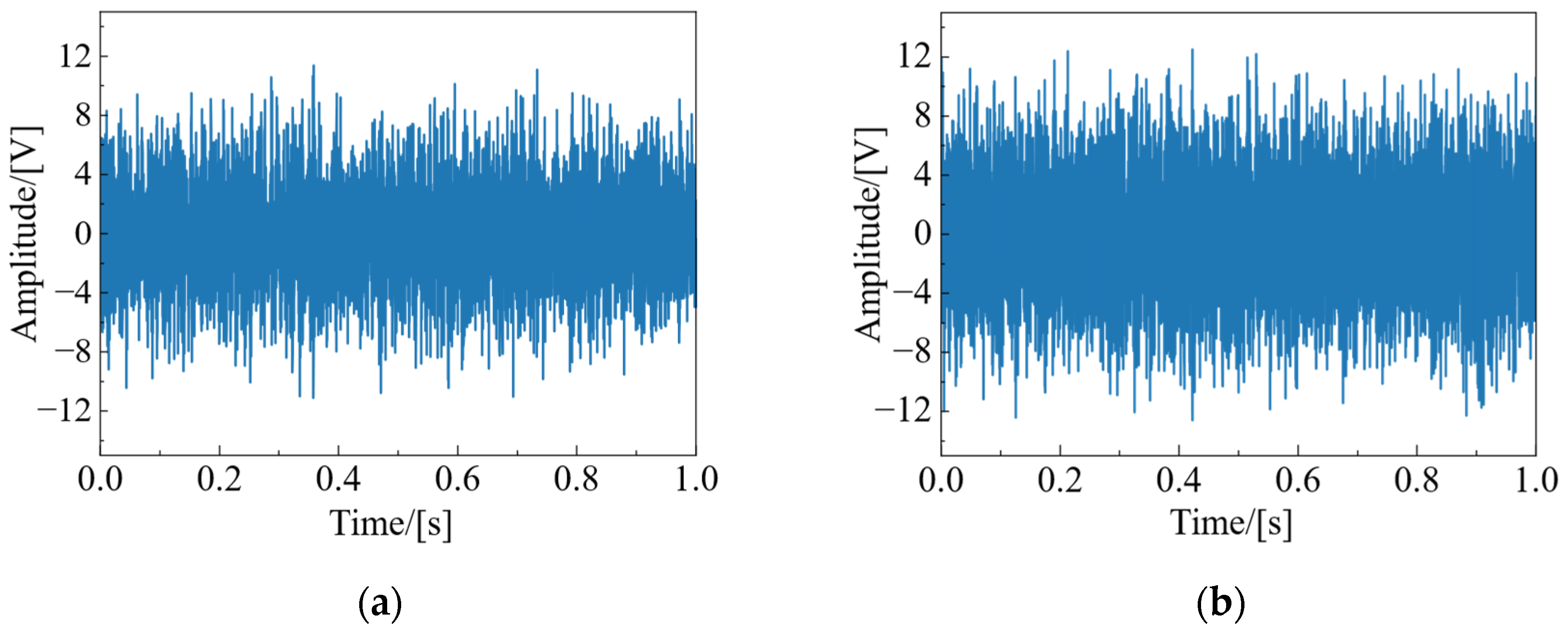
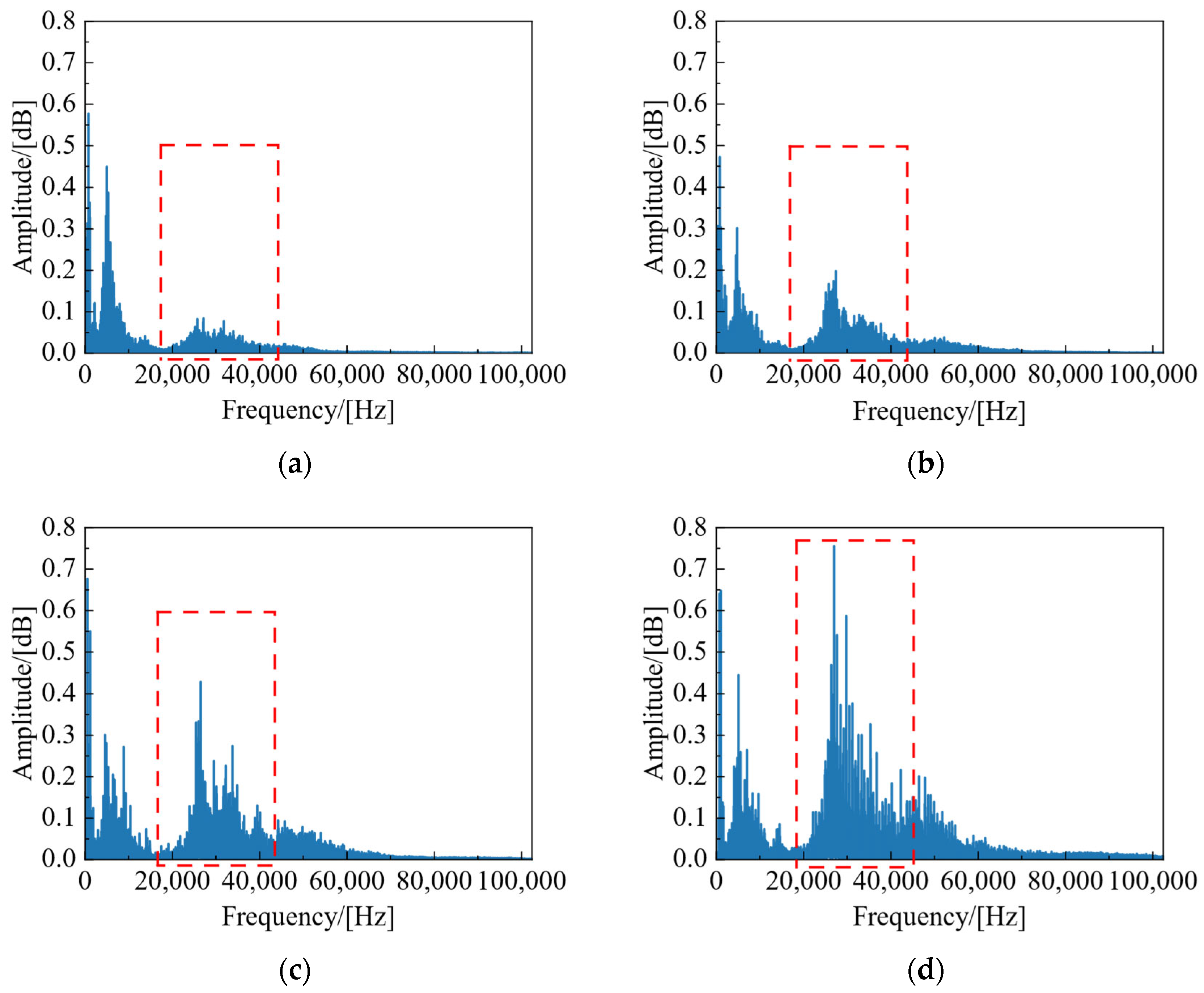
2.2.1. AE Data Analysis

AE data were analyzed to investigate the signal characteristics of bearing lubrication failure. As the test duration extended, the time-domain amplitude of the AE signals significantly increased. To better compare the AE amplitude values at different time points, four moments throughout the total duration were uniformly selected, as shown in Figure 3. This increase is due to the gradual loss of lubricant, leading to a reduction in oil film thickness, increased wear between the rolling elements and the inner and outer races, intensified AE events, and an increase in overall signal strength.

By processing the raw AE signals using FFT, we obtained the amplitude spectrum shown in Figure 4. The peaks observed in the AE data at frequencies of about 5–6 kHz and about 20–40 kHz may be caused by poor bearing lubrication. In the early stages of bearing lubrication failure, partial oil film rupture or the entry of contaminants can lead to rough contact between the rolling elements and the inner and outer raceways. This rough contact generates pulses and excites the natural frequencies of the bearing components, resulting in high-frequency vibration signals. This property is consistent with the conclusions presented in [26]. Therefore, this study focused on extracting features within this frequency range to enhance the correlation between the AE signals and the lubrication state.

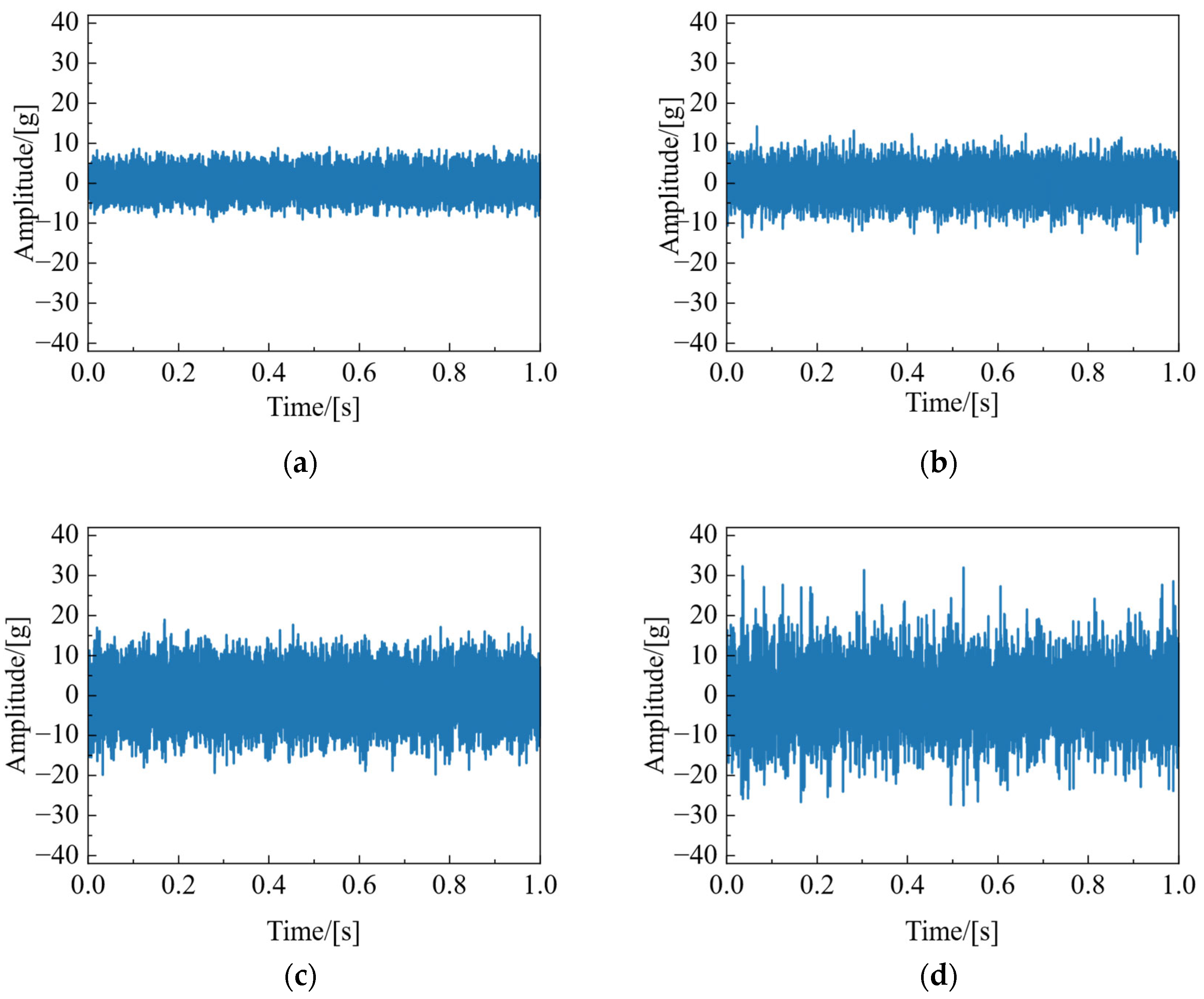
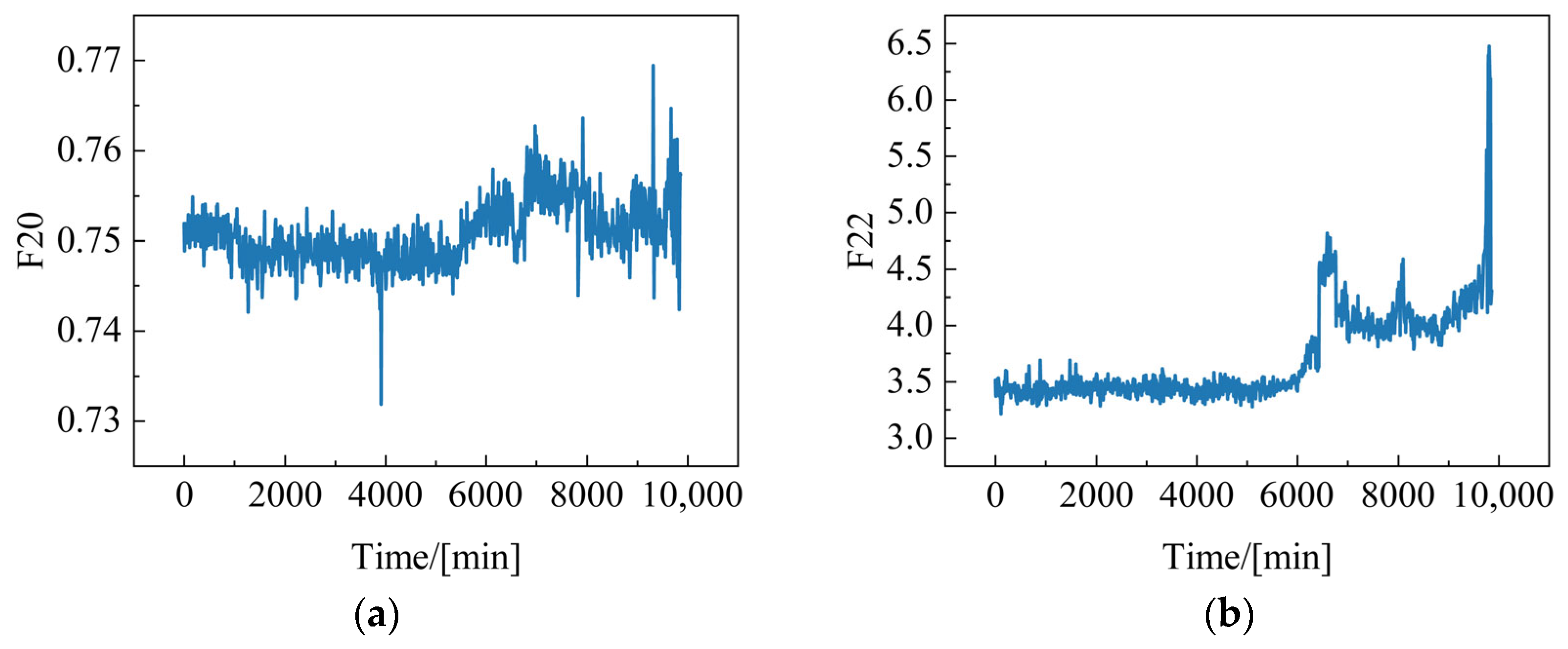
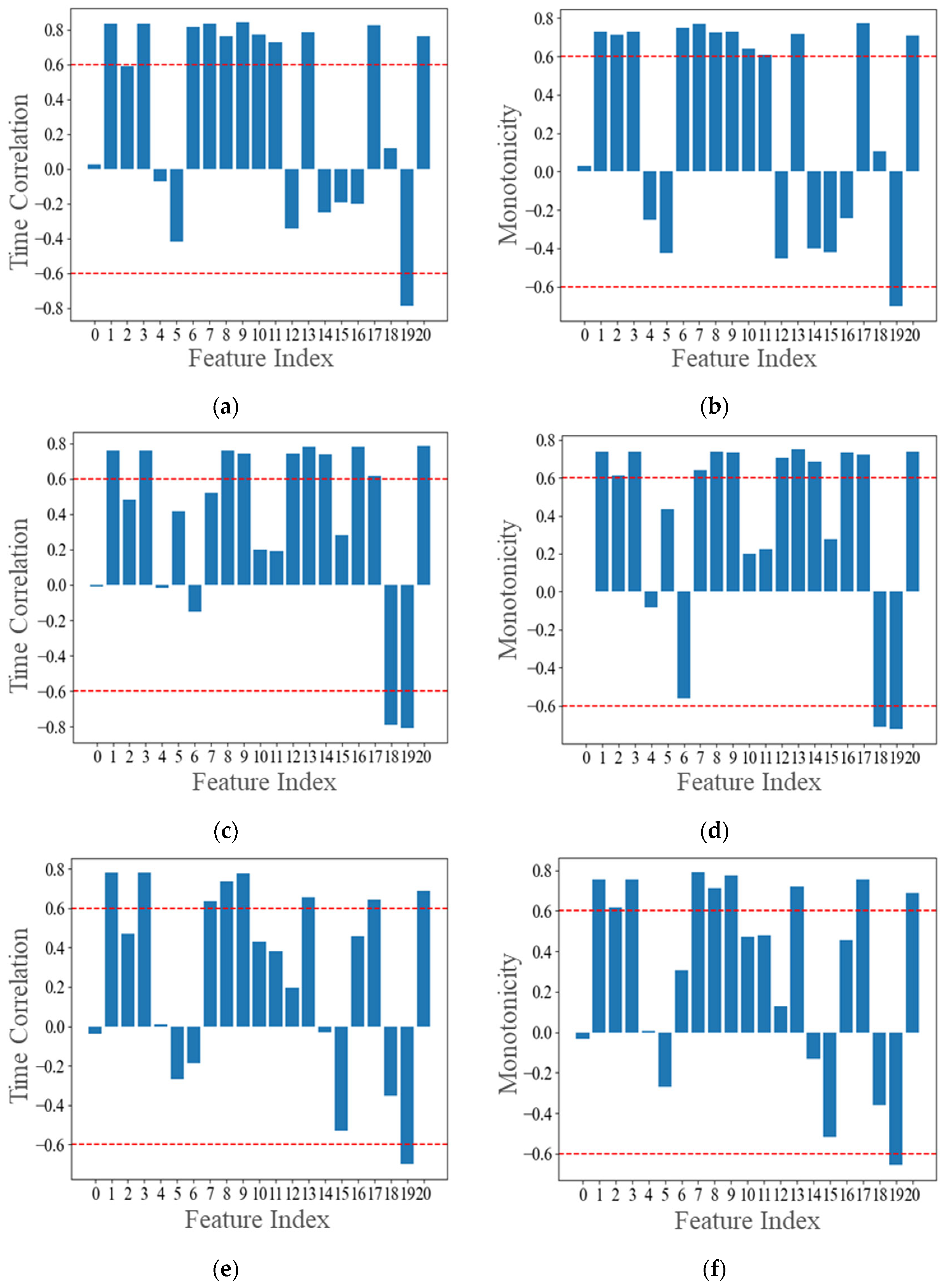
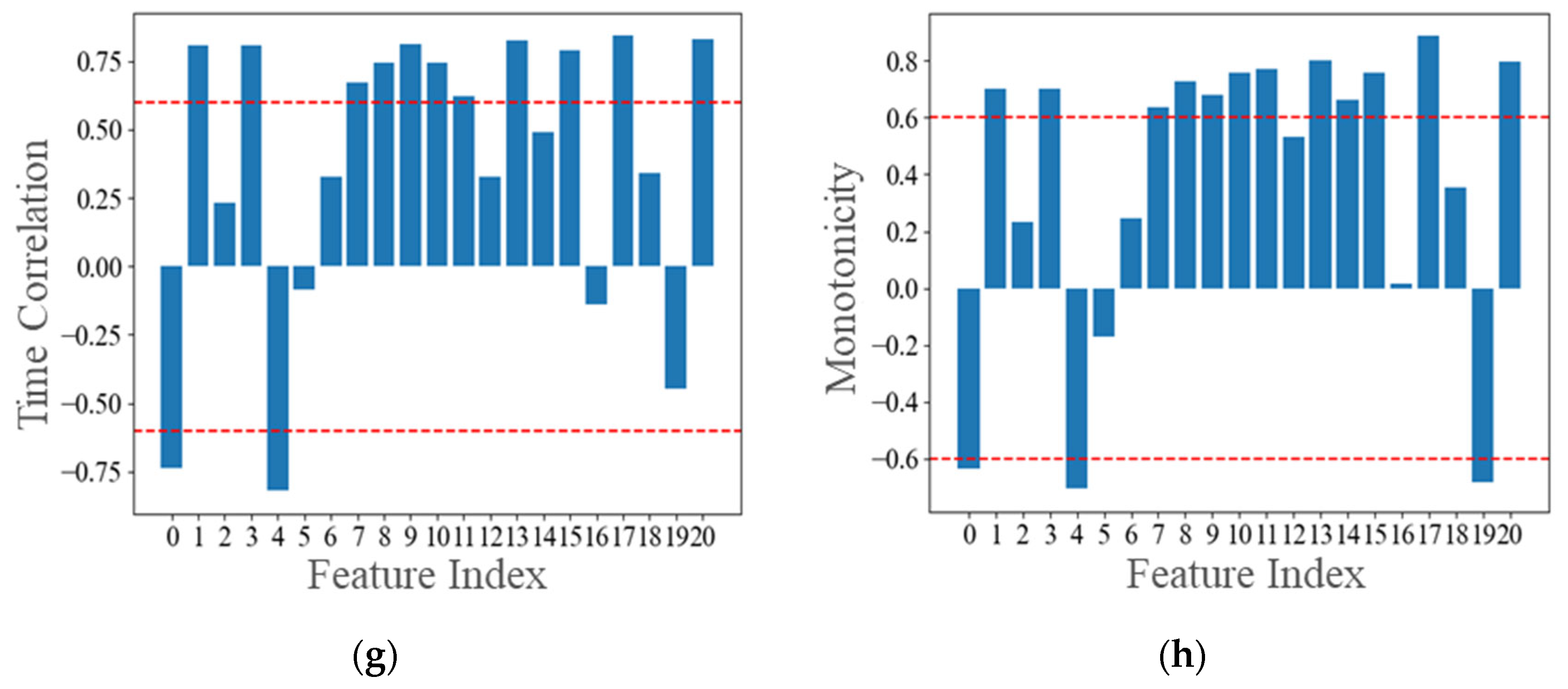
2.2.2. Vibration Data Analysis

Similarly, the vibration data were also analyzed to investigate the signal characteristics of bearing lubrication failure. It can be observed that the amplitude of the vibration signal significantly increased as the experiment progressed, indicating that the deterioration of lubrication directly affected the system’s vibration characteristics, as shown in Figure 5. This change is likely due to increased friction and wear caused by the deteriorating lubrication condition, leading to higher intensity and frequency of vibrations.

By processing the vibration signals using FFT, the amplitude spectrum, as shown in Figure 6, can be achieved. The figure shows that specific amplitude spectra are sensitive to the bearing lubrication degradation process. The vibration signal shows significant energy growth in the 0–3 kHz and 10–12.8 kHz frequency ranges, indicating that vibration signals can also reflect changes in the bearing’s lubrication state.

Low- and high-frequency spectral energy show varying degrees of increase, potentially indicating the impact of lubrication failure at different frequency ranges. Therefore, changes in vibration signals provide essential clues for identifying lubrication state degradation and early bearing faults.

2.2.3. Temperature Data Analysis

Insufficient lubrication results in extra friction and wear within bearings. As friction and wear are significant contributors to heat generation, monitoring temperature is thus a vital indicator for determining lubrication failure in bearings. Figure 7 shows the temperature variation during the last 1000 min of the experiment. It can be observed that before 9600 min, the bearing temperature remained relatively stable. However, after 9600 min, the temperature rose sharply. This is because, in the early stages of lubrication degradation, the oil loss is insufficient to cause a significant increase in friction. As lubrication conditions deteriorate progressively, tribological interactions and material degradation among bearing components intensify, culminating in a significant temperature spike. In contrast to the AE signal and vibration signal, the bearing temperature signal remained stable throughout the experimental phase, with a discernible change occurring after 9600 min. This also demonstrates that it is not appropriate to assess the bearing lubrication state solely based on the temperature signal as there is a certain lag in the temperature signal.

3. Materials and Methods

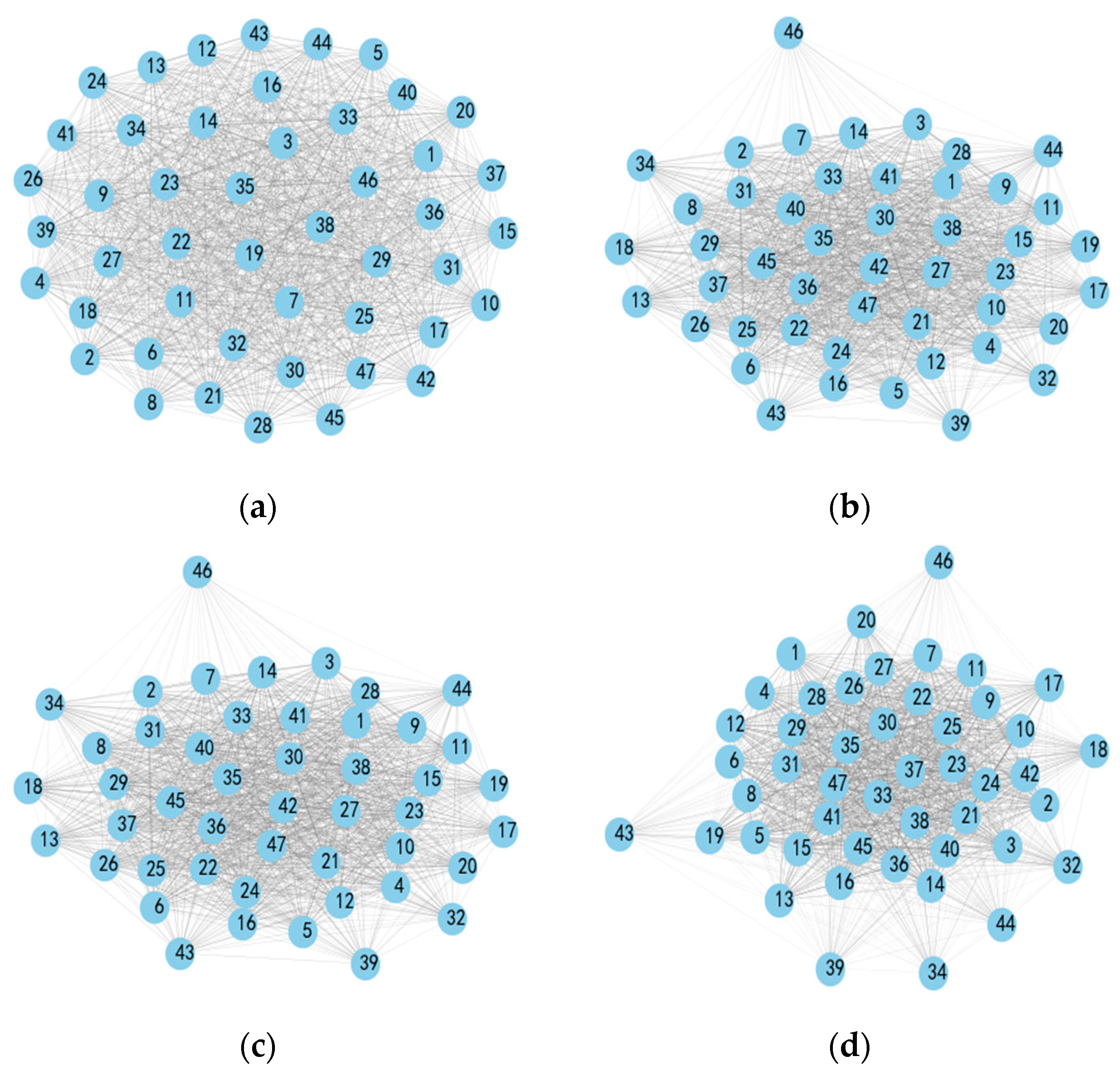
3.1. Construction of Graph Dataset Based on Prior Knowledge

Based on the analysis above, filtering procedures were applied to both the acoustic emission and vibration acceleration signals, followed by relevant feature extraction from the processed data. Notably, the frequency spectrum retained for the acoustic emission signal ranged from 20 kHz to 40 kHz, while for the vibration acceleration signal, frequency bands of 0–3 kHz and 10–12.8 kHz were preserved.

The signals’ detailed time-domain and frequency-domain features can be found in

Table 1. Features used for construction of graph data.

Feature	Equation	Feature	Equation
Mean	$\overline{x}=\frac{1}{N}x(i)$	Skewness	$S=\frac{{{\displaystyle {\sum }_{i=1}^N\left[x(i)-\overline{x}\right]}}^3}{(N-1){\sigma }_x^3}$
Standard Deviation	${\sigma }^x=\sqrt{\frac{1}{N-1}{{\displaystyle \sum _{i=1}^N\left[x(i)-\overline{x}\right]}}^2}$	Peak	$x_p=\max \left|x(i)\right|$
Root Mean Square	$x_{\mathrm{rms}}=\sqrt{\frac{1}{N}{\displaystyle \sum _{i=1}^N{x}^2}(i)}$	Kurtosis	$K=\frac{{{\displaystyle {\sum }_{i=1}^N\left[x(i)-\overline{x}\right]}}^4}{(N-1){\sigma }_x^4}$
Dominant Frequency	$F_{10}=\frac{\arg \max ({\left|\frac{s(k)}{K}\right|}^2)F_s}{K}$	Band-Specific Energy	$F_{11}={\displaystyle \sum _{k=0}^{3000}|s(k)}{|}^2$
Spectral Mean	$F_{12}=\frac{1}{K}{\displaystyle \sum _{k=1}^{K}s}(k)$	Spectra Standard Deviation	$F_{13}=\sqrt{\frac{1}{K-1}{{\displaystyle \sum _{k=1}^K\left[s(k)-F_{12}\right]}}^2}$
Spectral Skewness	$F_{14}=\frac{{\displaystyle \sum _{\mathrm{k}=1}^K{[s(k)-F_{12}]}^3}}{(K-1)F_{13}^3}$	Spectral Kurtosis	$F_{15}=\frac{{\displaystyle \sum _{\mathrm{k}=1}^K{[s(k)-F_{12}]}^4}}{(K-1)F_{13}^4}$
Center Frequency	$F_{16}=\frac{{\displaystyle \sum _{\mathrm{k}=1}^K{f}_k}\cdot s(k)}{{\displaystyle \sum _{k=1}^{K}s}(k)}$	Frequency-Weighted Standard Deviation	$F_{17}=\sqrt{\frac{1}{K-1}{\displaystyle \sum _{k=1}^K{\left(f_k-F_{16}\right)}^2}}$
Root Mean Square Frequency	$F_{18}=\sqrt{\frac{{\displaystyle \sum _{k=1}^K{f}_k^2\cdot s(k)}}{{\displaystyle \sum _{k=1}^{K}s(k)}}}$	Peak Frequency	$F_{19}=\sqrt{\frac{{\displaystyle \sum _{k=1}^K{f}_k^4\cdot s(k)}}{{\displaystyle \sum _{k=1}^K{f}_k^2\cdot s(k)}}}$
Spectral Flatness	$F_{20}=\frac{{\displaystyle \sum _{k=1}^K{f}_k^2}\cdot s(k)}{\sqrt{{\displaystyle \sum _{k=1}^{K}s}(k){\displaystyle \sum _{k=1}^K{f}_k^4}\cdot s(k)}}$	Normalized Frequency Standard Deviation	$F_{21}=\frac{F_{17}}{F_{16}}$
Frequency Skewness	$F_{22}=\frac{{\displaystyle \sum _{k=1}^K{\left(f_k-F_{16}\right)}^3}\cdot s(k)}{(K-1)F_{17}^3}$	Frequency Kurtosis	$F_{23}=\frac{{\displaystyle \sum _{k=1}^K{\left(f_k-F_{16}\right)}^4}\cdot s(k)}{(K-1)F_{17}^4}$
Normalized Bandwidth	$F_{24}=\frac{{\displaystyle \sum _{k=1}^K{\left(f_k-F_{16}\right)}^{1/2}}\cdot s(k)}{(K-1)F_{17}^{1/2}}$

$x\left(i\right)$ is the time-domain sequence of the signal, $i=\mathrm{1,2},3\cdots ,N$; $N$ is the number of samples; $F_s$ is the sampling frequency; $s\left(k\right)$ is the spectrum of the signal, $k=\mathrm{1,2},3\cdots ,K$; $K$ is the number of spectral lines; $f_k$ is the frequency value of the $k_{th}$ spectral line.

. Figure 8 illustrates some of the extracted features from the vibration signal.

Each second of the signal was analyzed and calculated separately to obtain the corresponding feature values. As shown in Figure 8, the vibration signals contain complex information, but some of the feature information does not reflect the trend of bearing lubrication degradation. Therefore, removing features that do not contain degradation trends is necessary.

Valuable features should demonstrate monotonicity and strong time correlation. Hence, this paper uses a comprehensive evaluation index based on monotonicity and time correlation as the criterion for feature selection [27,28], and the threshold of time correlation and monotonicity was set as 0.6.

Feature evaluation was conducted on the time-domain and frequency-domain features previously mentioned, as shown in Figure 9. The feature index corresponds sequentially to the time-domain and frequency-domain signals in Table 1.

Features that met both thresholds were selected, as shown in Figure 9, with their numbers corresponding sequentially to those in Table 1. Ultimately, a total of 46 features were selected for the AE and vibration signals. A detailed analysis of the AE and triaxial vibration signals identified 46 features indicative of bearing lubrication degradation trends. Only nine features from the vibration in the Z-direction were retained, suggesting that different types and directions of signals may hold varying sensitivity for this specific monitoring task. The temperature signal was included as an additional feature to examine further the impact of lubrication degradation on bearing temperature. As a result, the total number of time-series features describing bearing lubrication degradation was increased to 47.

Following the completion of the feature selection, the graph data construction was initiated. The experimental data consisted of 1000 data points spanning 10,000 min. The first 500 points were designated as the training dataset and contained only normal data, while the last 500 points were used as the test dataset and included some lubrication anomaly data. We first performed the maximum and minimum standardization operation for the original signal collected. The standardization process can be expressed as follows [29]:

$$X_{\mathrm{nol}}=\frac{X-X_{\min }}{X_{\max }-X_{\min }}$$

(1)

Subsequently, the monitoring data were processed using a sliding window technique with a window size of 30. The graph nodes were defined as the features of vibration, acoustic emission, and temperature signals. Each node was fully connected to every other node, with all edges initialized to have identical weights. The data vectors within each window were treated as the feature embedding vectors of a node. These vectors not only contained the state information of the current window but also implicitly reflected the local dynamic characteristics of the time series. The final graph data construction results are shown in the Figure 10.

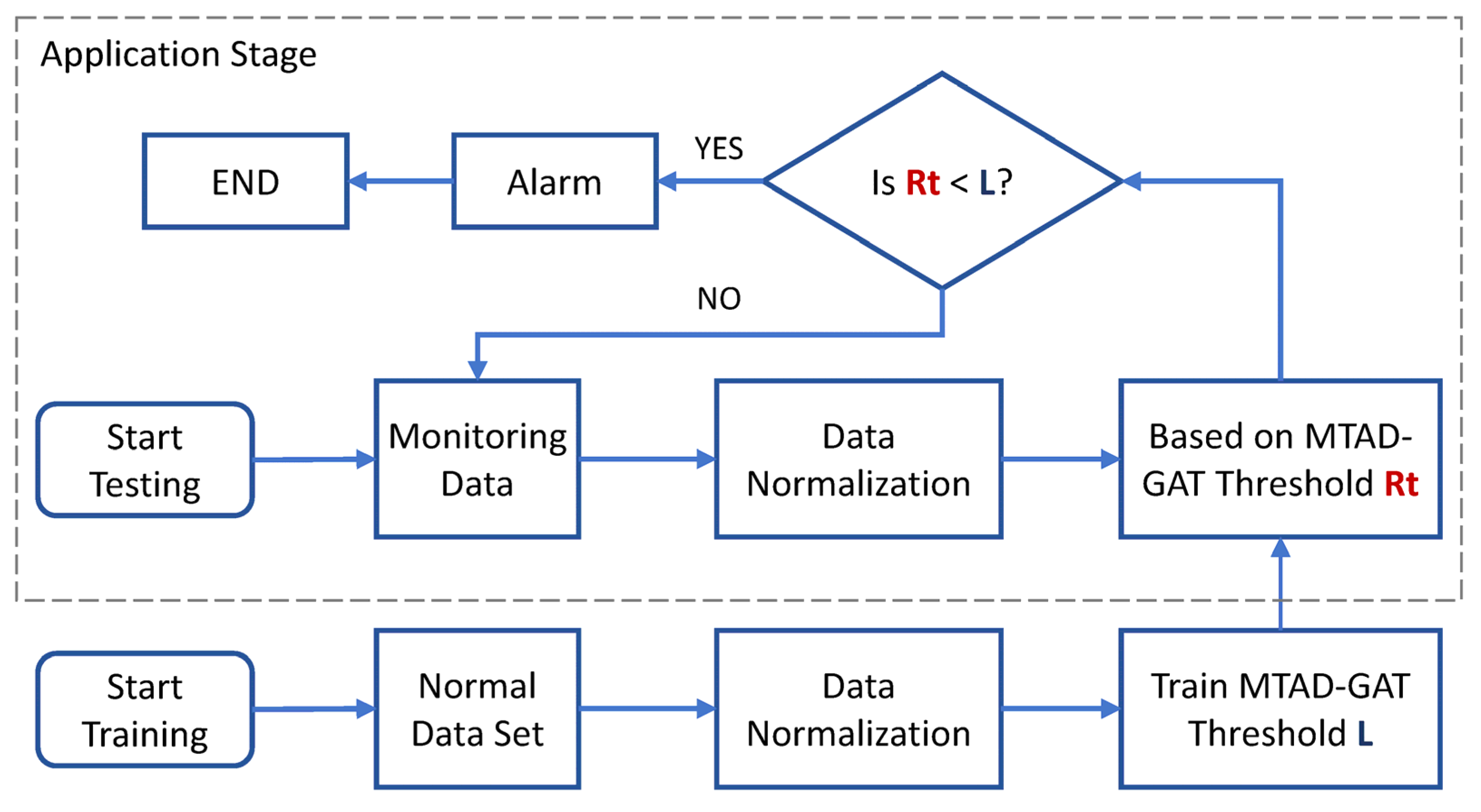
3.2. Lubrication Monitoring Process

Since this study focuses on the selection of sensors for bearing lubrication monitoring and the graph data construction process, we utilized an advanced graph model, MATD-GAT (multivariate time-series anomaly detection via graph attention network) [30], for subsequent anomaly diagnosis in bearing lubrication monitoring. Through in-depth analysis of time-series data, the model enhances accuracy in both prediction and reconstruction dimensions. Each layer was optimized for different aspects of time-series analysis, enabling the model to capture the complexity of time-series data effectively. The detailed steps for monitoring bearing lubrication conditions are shown in Figure 11.

4. Discussion

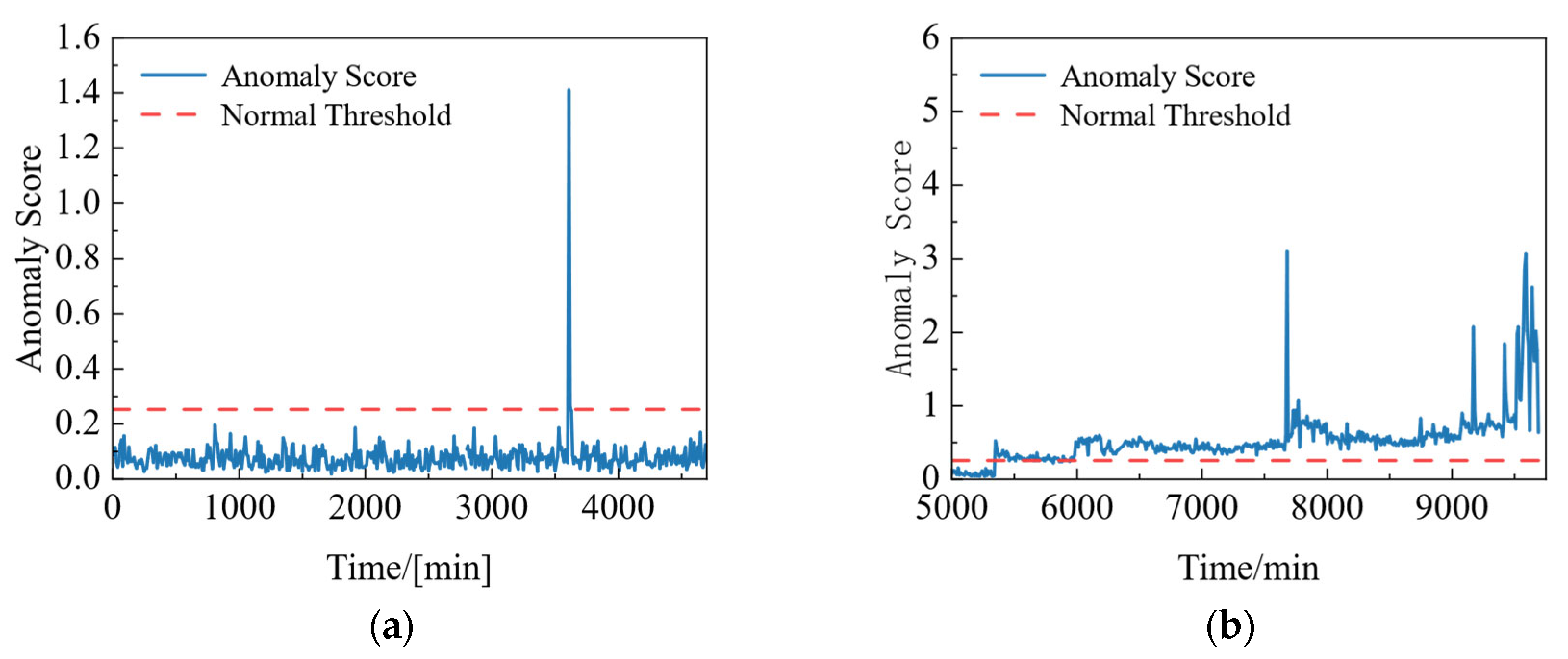
4.1. Lubrication Failure Monitoring

In the initial stages of training, the coupling relationships between nodes were unclear. As the training progressed, these relationships became more apparent, indicating that the model was learning deeper structural information and feature interactions. Figure 12 shows the fusion weights between different nodes. From the figure, it can be seen that as training proceeds, the width of the edges between nodes shifts from an even distribution to varying thicknesses between some nodes, and the relative positions of the nodes gradually change. Strongly correlated nodes start clustering together, while weakly correlated nodes move apart.

To achieve accurate condition monitoring, the monitoring model needs to detect the early degradation onset point of the equipment accurately. This point represents the critical transition from normal operation to the onset of degradation. Before this point, the equipment operates normally; beyond that, it begins to experience lubrication degradation and other faults. The monitoring results using three vibration sensor signals, an AE signal, and a temperature signal are shown in Figure 13.

Analysis results show that the anomaly scores remain stable during the model training. The model ultimately sets the normal threshold at 0.31. Anomalous data may cause the significant peaks observed in Figure 13a. The timing of these anomalies was close to when the bearing began to degrade, which could be due to the temporary rupture of the oil film in the contact area. Subsequently, the oil film of the bearing recovered, and the significant peaks disappeared. Bearing lubrication degradation test data revealed that after 5300 min, the anomaly scores surpassed the normal threshold, indicating that the bearing entered the degradation phase, as shown in Figure 13b. After 5300 min, the anomaly scores gradually increased, corresponding to the bearing’s degradation process. This finding indicates that the developed condition monitoring model is highly sensitive to early abnormal states and can accurately detect lubrication status.

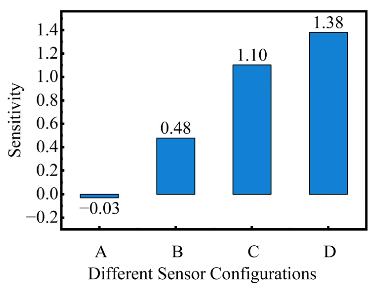
4.2. Impact of Sensor Missing

To investigate the impact of a missing sensor on bearing lubrication monitoring, experiments were conducted. These experiments involved using partial sensor data to monitor lubrication anomalies. The following configurations were tested: using only single vibration data, using one vibration data and one acoustic emission data, and using two vibration data and one acoustic emission data to evaluate the model’s effectiveness in detecting lubrication anomalies.

Figure 14 shows the detection results when the model was trained using only one vibration sensor signal. The anomaly scores obtained from training the model with normal data are shown in Figure 14a, with a normal threshold set at 0.25. The model trained with a test set containing degradation trends is shown in Figure 14b. The normal threshold can be used to distinguish between normal and abnormal states of the system. However, the anomaly scores around the degradation point were approximately 0.3, as shown in Figure 14b, which is close to the normal threshold. Therefore, using only one vibration sensor to monitor bearing lubrication status is unsuitable.

Figure 15 shows the detection results when the model was trained using one vibration sensor and one acoustic emission signal. The anomaly scores obtained from training the model with normal data are shown in Figure 15a, with a normal threshold set at 0.33. The model trained with a test set containing degradation trends is shown in Figure 15b. It can be seen that using the vibration sensor data and acoustic emission signals for model training results in a more distinct separation between anomaly scores in normal and abnormal states. The anomaly scores for early abnormal states were around 1.2, indicating an improved distinction between normal and abnormal states.

Figure 16 shows the detection results when the model was trained using two vibration sensors and one acoustic emission signal. The anomaly scores obtained from training the model with normal data are shown in Figure 16a, with a normal threshold set at 0.28. The model trained with a test set containing degradation trends is shown in Figure 16b. It can be seen that using two vibration sensors and one acoustic emission signal for model training results in an even more distinct separation between anomaly scores in normal and abnormal states. The anomaly scores for early abnormal states were around 1.6, further improving the distinction between normal and abnormal states.

The minimum difference between the anomaly score during the anomaly phase and the normal threshold was used as the sensitivity indicator to quantify the effect of the sensor missing on lubrication anomaly monitoring. A more significant difference indicates that the model is more sensitive in distinguishing between normal and abnormal data. Figure 17 shows the sensitivity of lubrication failure monitoring under different sensor missing conditions: single vibration data (A), one vibration data and acoustic emission data (B), two vibration data and one acoustic emission data (C), and three vibration data, acoustic emission data, and temperature data (D). The results indicate that the monitoring effect was poorest when using a single vibration data, with some anomalies undetected. With the increase in signal types and quantities, the model’s detection sensitivity progressively was enhanced. The best detection results were achieved with input from three vibration, acoustic emission, and temperature sensors. These results underscore the necessity of using multi-source sensors for effective lubrication status monitoring.

5. Conclusions

In this paper, a bearing lubrication failure simulation experiment was designed. The bearing’s temperature, acoustic emission, and vibration data were collected during the failure process to establish a dataset for the bearing lubrication failure process. Based on prior knowledge, feature selection was performed on the dataset to obtain time-series features that describe bearing lubrication degradation. Subsequently, using the above features as nodes, a bearing lubrication failure graph data was established. The MTAD-GAT model was used to research abnormal lubrication state monitoring and the impact of sensor loss, leading to the following conclusions:

• During the bearing lubrication degradation process, acoustic emission, vibration, and temperature signals can all respond to bearing lubrication failure, but the temperature signal exhibits a certain lag;
• The monitoring model trained on graph data constructed based on prior knowledge is susceptible to early abnormal states and can accurately capture early degradation signals of the bearing lubrication state;
• In the absence of sensor signals, monitoring results using only vibration data exhibit a certain lag. With the increase in signal types and quantities, the model’s detection sensitivity gradually increases, proving the necessity of using multi-source sensors in bearing lubrication state monitoring.

Based on the above discussion, it is evident that multi-sensor graph data hold significant potential for bearing lubrication state monitoring. However, the application of multiple sensors reduces the robustness of the bearing lubrication monitoring system. Future work will involve more diverse sensor data and address potential sensor fault diagnostics.

References

1. Xu, F.; Ding, N.; Li, N.; Liu, L.; Hou, N.; Xu, N.; Guo, W.; Tian, L.; Xu, H.; Wu, C.-M.L.; et al. A Review of Bearing Failure Modes, Mechanisms and Causes. Eng. Fail. Anal. 2023, 152, 107518. [Google Scholar] [CrossRef]
2. de Azevedo, H.D.M.; Araújo, A.M.; Bouchonneau, N. A Review of Wind Turbine Bearing Condition Monitoring: State of the Art and Challenges. Renew. Sustain. Energy Rev. 2016, 56, 368–379. [Google Scholar] [CrossRef]
3. Yang, Z.; Niu, X.; Li, C.; Zhou, N. Experimental Investigation of the Influence of the Pocket Shape on the Cage Stability of High-Precision Ball Bearings. Precis. Eng. 2023, 82, 62–67. [Google Scholar] [CrossRef]
4. NSK. Machine Tool Spindle Bearing Selection & Mounting Guide; Motion & Control NSK: Maynila, Philippines, 2009. [Google Scholar]
5. Takegahana, J.; Koyama, M.; Jinno, K. Angular Contact Ball Bearings for High-Speed and Heavy-Cutting Machine Tools. NTN Tech. Rev. 2018, 56–61. Available online: https://www.ntnglobal.com/en/products/review/pdf/NTN_TR86_en.pdf (accessed on 18 June 2024).
6. Chang, Z.; Jia, Q.; Yuan, X.; Chen, Y. Main Failure Mode of Oil-Air Lubricated Rolling Bearing Installed in High Speed Machining. Tribol. Int. 2017, 112, 68–74. [Google Scholar] [CrossRef]
7. Lugt, P.M. Grease Lubrication in Rolling Bearings; John Wiley & Sons: Hoboken, NJ, USA, 2012. [Google Scholar]
8. Jakobsen, M.O.; Herskind, E.S.; Pedersen, C.F.; Knudsen, M.B. Detecting Insufficient Lubrication in Rolling Bearings, Using a Low Cost MEMS Microphone to Measure Vibrations. Mech. Syst. Signal Process. 2023, 200, 110553. [Google Scholar] [CrossRef]
9. He, Y.; Li, M.; Meng, Z.; Chen, S.; Huang, S.; Hu, Y.; Zou, X. An Overview of Acoustic Emission Inspection and Monitoring Technology in the Key Components of Renewable Energy Systems. Mech. Syst. Signal Process. 2021, 148, 107146. [Google Scholar] [CrossRef]
10. Tiboni, M.; Remino, C.; Bussola, R.; Amici, C. A Review on Vibration-Based Condition Monitoring of Rotating Machinery. Appl. Sci. 2022, 12, 972. [Google Scholar] [CrossRef]
11. Mobil. Guide to Electric Motor Bearing Lubrication. 2009. Available online: https://www.mobil.com/lubricants/-/media/files/global/us/industrial/tech-topics/tt-electric-motor-bearing-lubrication-guide.pdf (accessed on 18 June 2024).
12. Xu, X.; Liao, X.; Zhou, T.; He, Z.; Hu, H. Vibration-Based Identification of Lubrication Starved Bearing Using Spectral Centroid Indicator Combined with Minimum Entropy Deconvolution. Measurement 2024, 226, 114156. [Google Scholar] [CrossRef]
13. Miettinen, J.; Andersson, P.; Wikströ, V. Analysis of Grease Lubrication of a Ball Bearing Using Acoustic Emission Measurement. Proc. Inst. Mech. Eng. Part J J. Eng. Tribol. 2001, 215, 535–544. [Google Scholar] [CrossRef]
14. Yoshioka, T.; Shimizu, S. Monitoring of Ball Bearing Operation under Grease Lubrication Using a New Compound Diagnostic System Detecting Vibration and Acoustic Emission. Tribol. Trans. 2009, 52, 725–730. [Google Scholar] [CrossRef]
15. Fan, Y.E.; Shi, Z.; Harris, G.; Gu, F.; Ball, A. Monitoring the Lubrication Condition of Rolling Element Bearings Using the Acoustic Emission Technique. In Proceedings of the ASME 8th Biennial Conference on Engineering Systems Design and Analysis, Torino, Italy, 4–7 July 2006; Volume 42495, pp. 843–848. [Google Scholar]
16. Krishnamoorthy, V.; Anitha John, A.; Bhaumik, S.; Paleu, V. Mapping Acoustic Frictional Properties of Self-Lubricating Epoxy-Coated Bearing Steel with Acoustic Emissions during Friction Test. Technologies 2024, 12, 30. [Google Scholar] [CrossRef]
17. Wang, Z.; Wu, Z.; Li, X.; Shao, H.; Han, T.; Xie, M. Attention-Aware Temporal–Spatial Graph Neural Network with Multi-Sensor Information Fusion for Fault Diagnosis. Knowl.-Based Syst. 2023, 278, 110891. [Google Scholar] [CrossRef]
18. Huang, J.; Cui, L. Tensor Singular Spectrum Decomposition: Multisensor Denoising Algorithm and Application. IEEE Trans. Instrum. Meas. 2023, 72, 1–15. [Google Scholar] [CrossRef]
19. Meng, Z.; Zhu, J.; Cao, S.; Li, P.; Xu, C. Bearing Fault Diagnosis under Multisensor Fusion Based on Modal Analysis and Graph Attention Network. IEEE Trans. Instrum. Meas. 2023, 72, 1–10. [Google Scholar] [CrossRef]
20. Zhang, X.; Zhang, X.; Liu, J.; Wu, B.; Hu, Y. Graph Features Dynamic Fusion Learning Driven by Multi-Head Attention for Large Rotating Machinery Fault Diagnosis with Multi-Sensor Data. Eng. Appl. Artif. Intell. 2023, 125, 106601. [Google Scholar] [CrossRef]
21. Du, X.; Yu, J. Graph Neural Network-Based Early Bearing Fault Detection. arXiv 2022, arXiv:2204.11220. [Google Scholar]
22. Kenning, M.; Deng, J.; Edwards, M.; Xie, X. A Directed Graph Convolutional Neural Network for Edge-Structured Signals in Link-Fault Detection. Pattern Recognit. Lett. 2022, 153, 100–106. [Google Scholar] [CrossRef]
23. Zhao, X.; Yao, J.; Deng, W.; Ding, P.; Zhuang, J.; Liu, Z. Multiscale Deep Graph Convolutional Networks for Intelligent Fault Diagnosis of Rotor-Bearing System under Fluctuating Working Conditions. IEEE Trans. Ind. Inform. 2022, 19, 166–176. [Google Scholar] [CrossRef]
24. Zheng, H.; Ma, M.; Wen, B.; Zeng, Z.; Liu, W. Network Intrusion Anomaly Detection with GATv2. Front. Data Comput. 2024, 6, 179–190. [Google Scholar]
25. Yu, Z.; Zhang, C.; Deng, C. An Improved GNN Using Dynamic Graph Embedding Mechanism: A Novel End-to-End Framework for Rolling Bearing Fault Diagnosis under Variable Working Conditions. Mech. Syst. Signal Process. 2023, 200, 110534. [Google Scholar] [CrossRef]
26. Cockerill, A.; Clarke, A.; Pullin, R.; Bradshaw, T.; Cole, P.; Holford, K.M. Determination of Rolling Element Bearing Condition via Acoustic Emission. Proc. Inst. Mech. Eng. Part J J. Eng. Tribol. 2016, 230, 1377–1388. [Google Scholar] [CrossRef]
27. Mao, W.; He, J.; Zuo, M.J. Predicting Remaining Useful Life of Rolling Bearings Based on Deep Feature Representation and Transfer Learning. IEEE Trans. Instrum. Meas. 2019, 69, 1594–1608. [Google Scholar] [CrossRef]
28. Coble, J.; Hines, J.W. Applying the General Path Model to Estimation of Remaining Useful Life. Int. J. Progn. Health Manag. 2011, 2, 71. [Google Scholar] [CrossRef]
29. Lei, J.; Liu, C.; Jiang, D. Fault Diagnosis of Wind Turbine Based on Long Short-Term Memory Networks. Renew. Energy 2019, 133, 422–432. [Google Scholar] [CrossRef]
30. Zhao, H.; Wang, Y.; Duan, J.; Huang, C.; Cao, D.; Tong, Y.; Xu, B.; Bai, J.; Tong, J.; Zhang, Q. Multivariate Time-Series Anomaly Detection via Graph Attention Network. In Proceedings of the 2020 IEEE International Conference on Data Mining (ICDM), Sorrento, Italy, 17–20 November 2020; IEEE: New York, NY, USA, 2020; pp. 841–850. [Google Scholar]
Figure 1. Bearing Prognostics Simulator: 1—oil distribution system; 2—motor; 3—support shaft; 4—support bearing; 5—test bearing; 6—hydraulic load controls; 7—tachometer; 8—AC VFD motor controller.
Lubricants 12 00229 g001
Figure 2. Test bearing housing with sensors: (a) schematic diagram of test bearing installation; (b) actual picture of the test bearing and sensors.
Lubricants 12 00229 g002
Figure 3. The raw AE signal of test bearing: (a) after 2520 min; (b) after 5040 min; (c) after 7560 min; and (d) after 10,080 min.
Lubricants 12 00229 g003aLubricants 12 00229 g003b
Figure 4. The amplitude spectrums of AE signals: (a) after 2520 min; (b) after 5040 min; (c) after 7560 min; and (d) after 10,080 min.
Lubricants 12 00229 g004
Figure 5. The raw vibration signals of the test bearing: (a) after 2520 min; (b) after 5040 min; (c) after 7560 min; and (d) after 10,080 min.
Lubricants 12 00229 g005
Figure 6. The amplitude spectrums of vibration signals: (a) after 2520 min; (b) after 5040 min; (c) after 7560 min; and (d) after 10,080 min.
Lubricants 12 00229 g006
Figure 7. Test bearing temperature data.
Lubricants 12 00229 g007
Figure 8. Features of vibration signals: (a) spectral skewness; (b) center frequency.
Lubricants 12 00229 g008
Figure 9. Feature evaluation: (a) Time correlation of vibration in the X-direction; (b) monotonicity of vibration in the X-direction; (c) time correlation of vibration in the Y-direction; (d) monotonicity of vibration in the Y-direction; (e) time correlation of vibration in the Z-direction; (f) monotonicity of vibration in the Z-direction; (g) time correlation of the AE signal; (h) monotonicity of the AE signal.
Lubricants 12 00229 g009aLubricants 12 00229 g009b
Figure 10. Results of graph data construction.
Lubricants 12 00229 g010
Figure 11. Bearing lubrication condition monitoring process.
Lubricants 12 00229 g011
Figure 12. Visualization of the graph data training process: (a) graph structure of epoch 0; (b) graph structure of epoch 50; (c) graph structure of epoch 100; (d) graph structure of epoch 150.
Lubricants 12 00229 g012
Figure 13. Monitoring results of lubrication degradation data: (a) anomaly score of the train dataset; (b) anomaly score of the test dataset.
Lubricants 12 00229 g013
Figure 14. Monitoring results of lubrication degradation using only single vibration data: (a) anomaly score of the train dataset; (b) anomaly score of the test dataset.
Lubricants 12 00229 g014
Figure 15. Monitoring results of lubrication degradation using one vibration data and one acoustic emission data: (a) anomaly score of the training dataset; (b) anomaly score of the test dataset.
Lubricants 12 00229 g015
Figure 16. Monitoring results of lubrication degradation using two vibration data and one acoustic emission data: (a) anomaly score of the training dataset; (b) anomaly score of the test dataset.
Lubricants 12 00229 g016
Figure 17. Sensitivity indicator of different configurations.
Lubricants 12 00229 g017