Numerical Simulations and Experimental Validation of Squeeze Film Dampers for Aircraft Jet Engines

 , , , and
Abstract
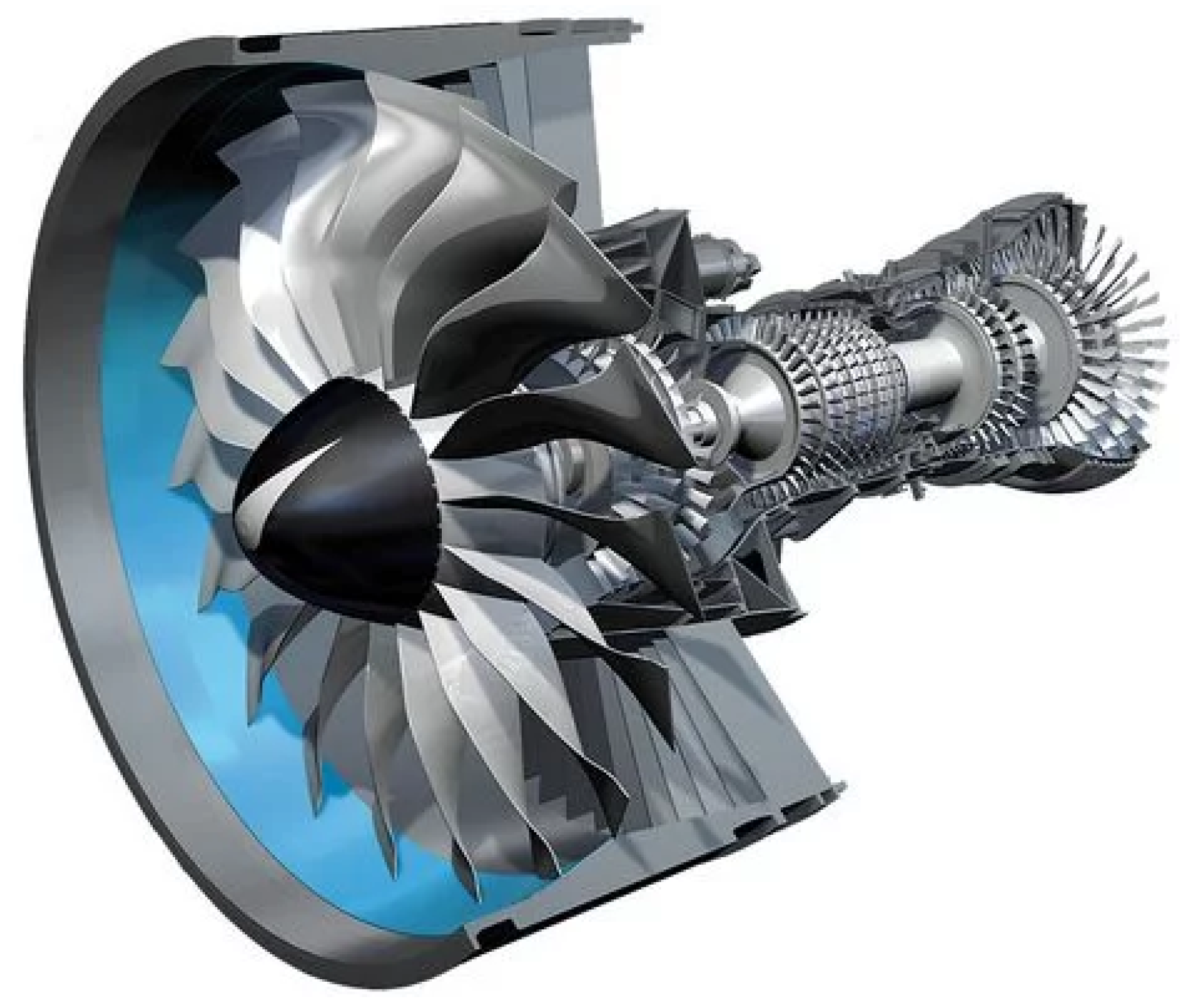
:1. Introduction
- A special experimental setup is presented that can be used to validate the SFD bearing forces for all operating conditions that may occur in an aircraft jet engine.
- The SFD bearing forces obtained from the experimental results are compared with those obtained from the numerical simulations and a good agreement is found.
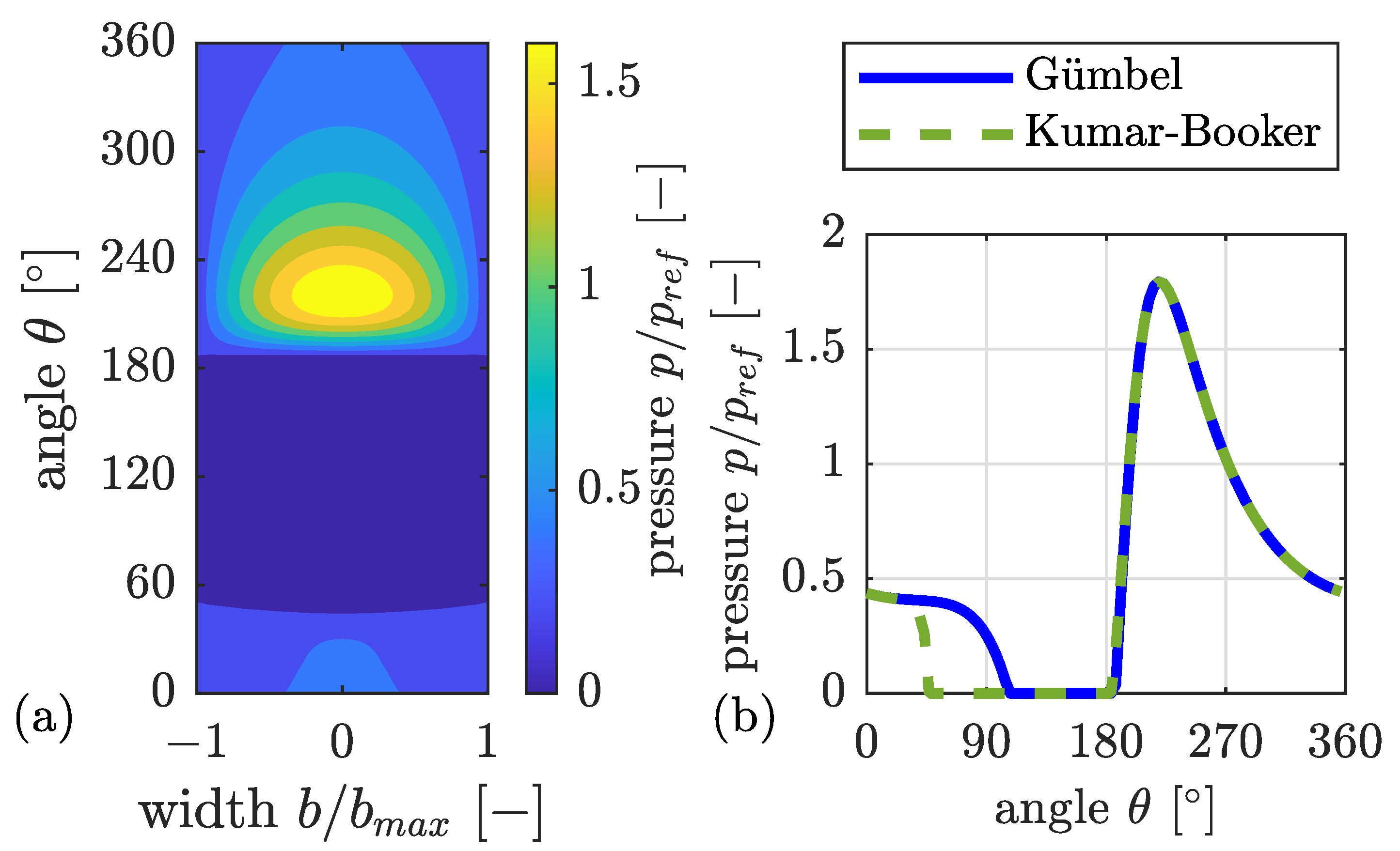
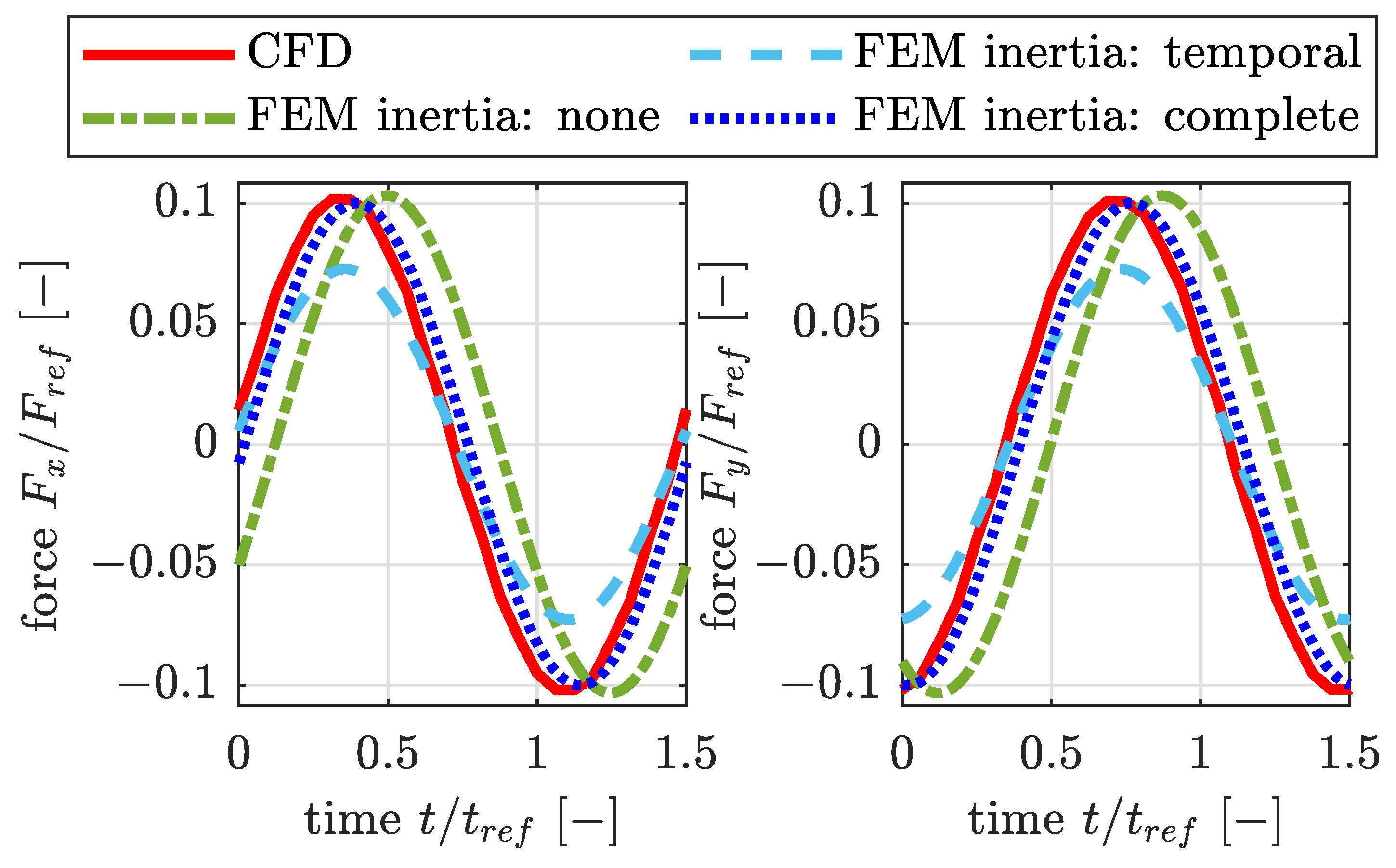
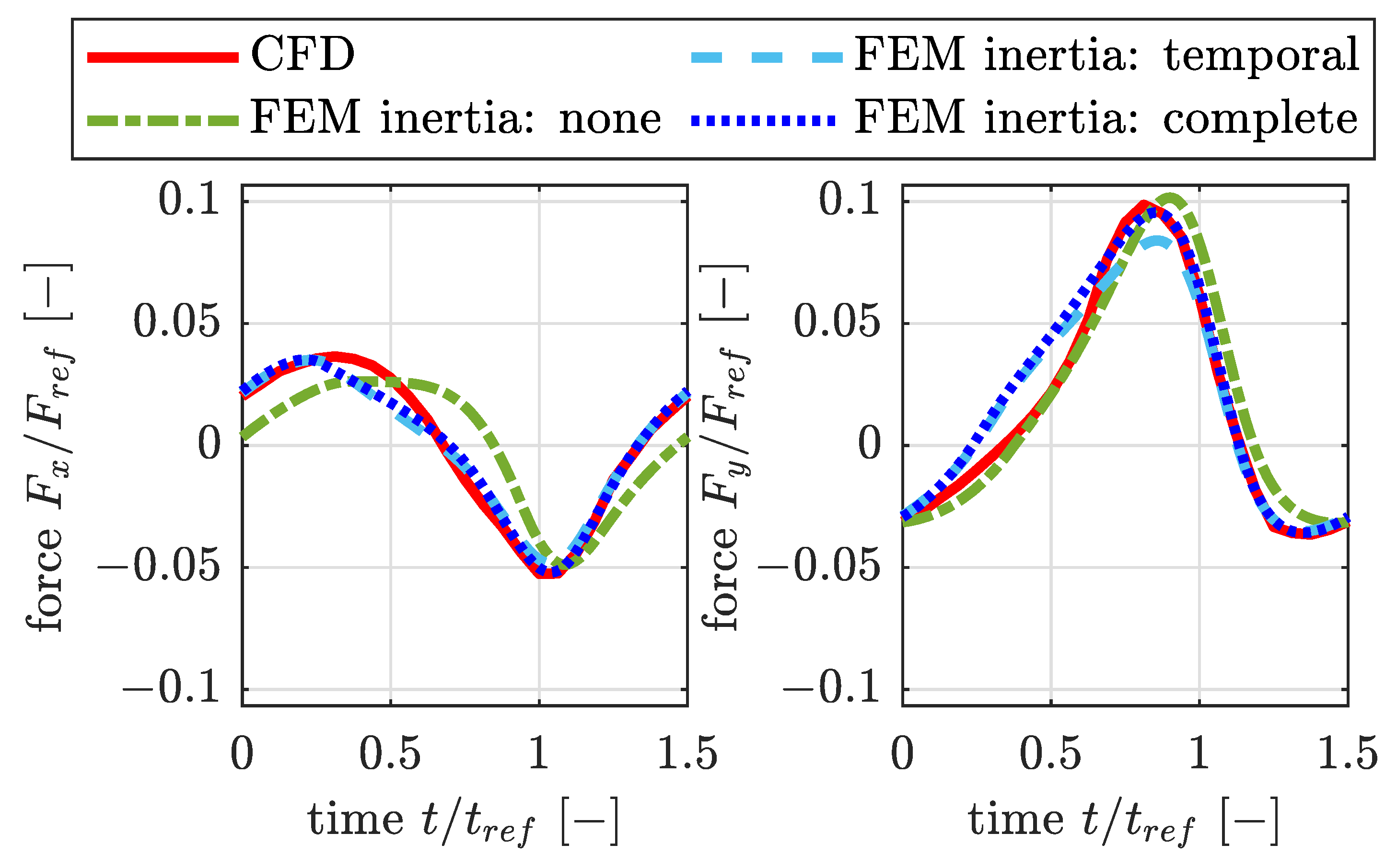
- The 2D solution of the Reynolds equation is compared with a 3D-CFD solution for thin-film lubrication conditions. The influence of inertia effects is shown to be significant for the specific parameter used.
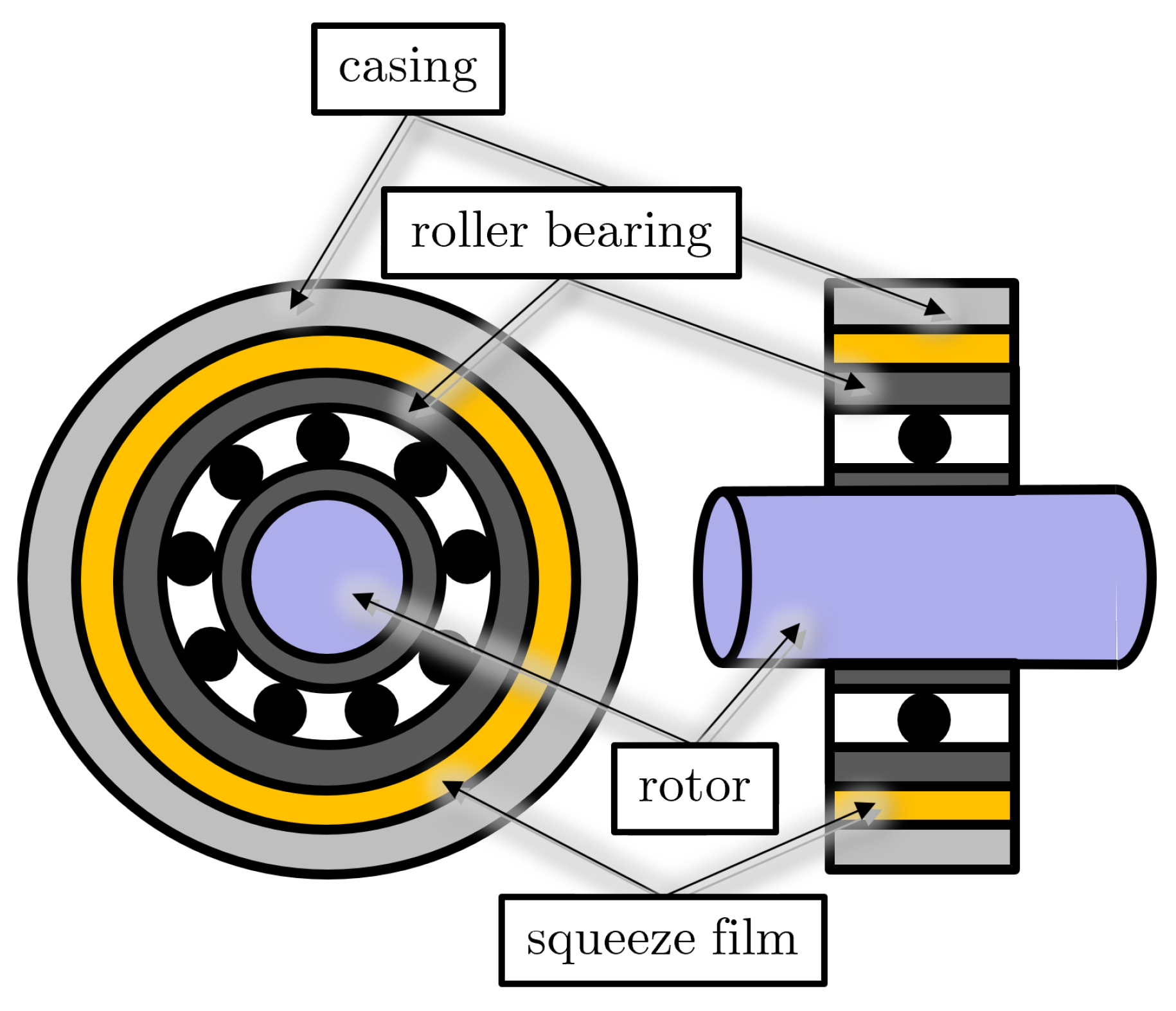
2. Hydrodynamic Lubrication in Squeeze Film Dampers
2.1. Thermo-Hydrodynamic Modeling
2.1.1. Generalized Reynolds Equation with a Mass-Conserving Cavitation Algorithm
- Region 1a (, );
- Region 1b (, );
- Region 2 ().
2.1.2. Temporal and Convective Inertia in the Reynolds Equation
2.1.3. Energy Equation in the Oil Film
2.2. Finite Element Formulation of the Thermo-Hydrodynamic Equations
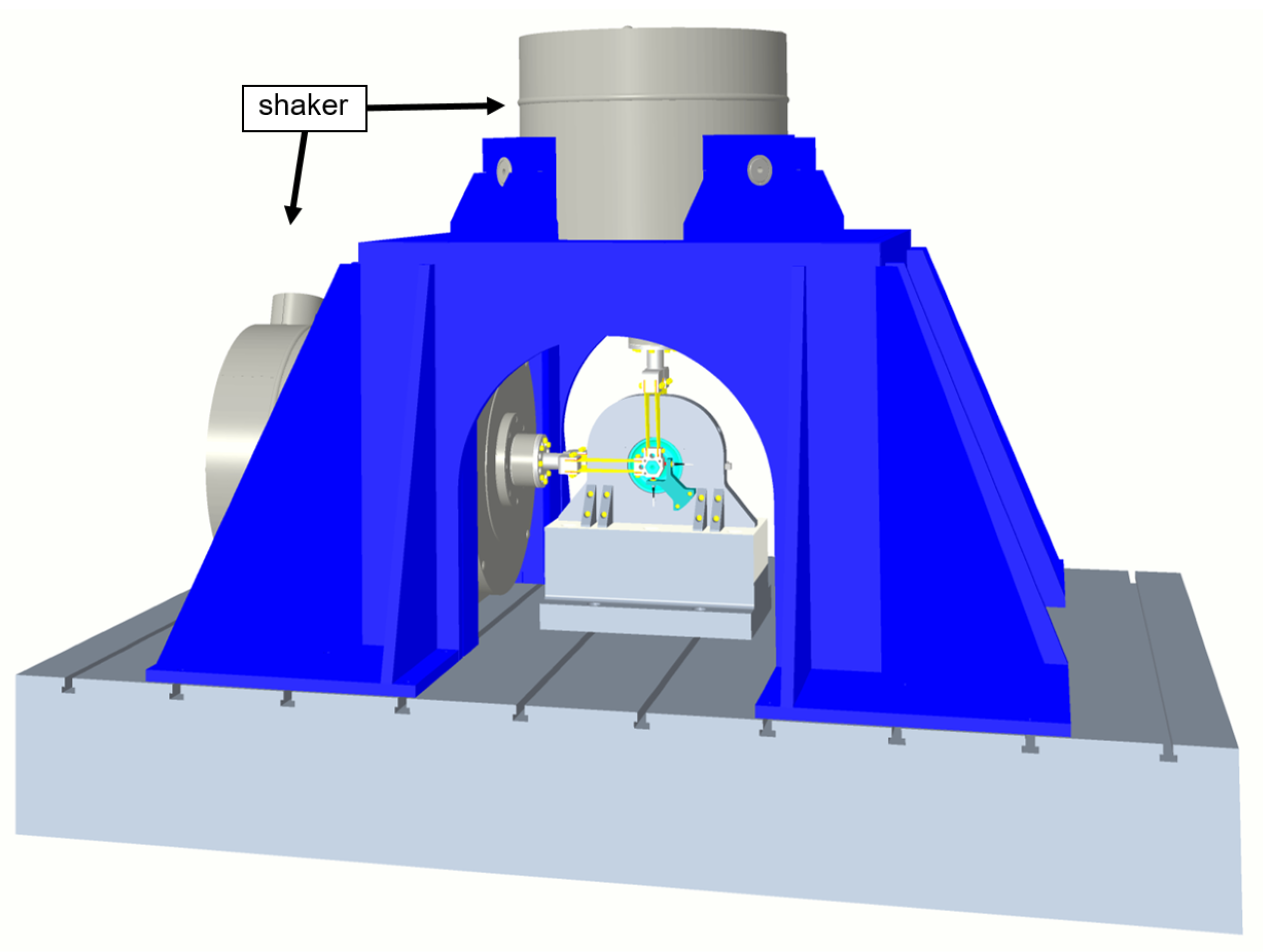
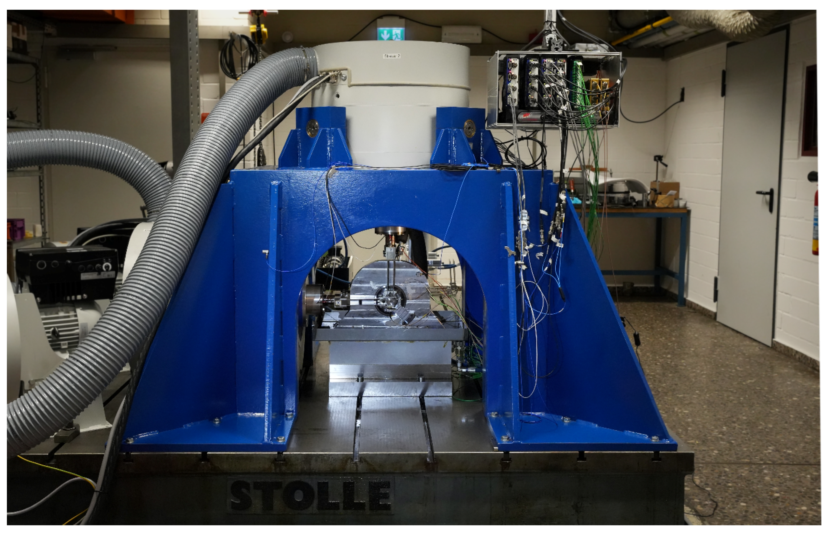
3. Experimental Setup
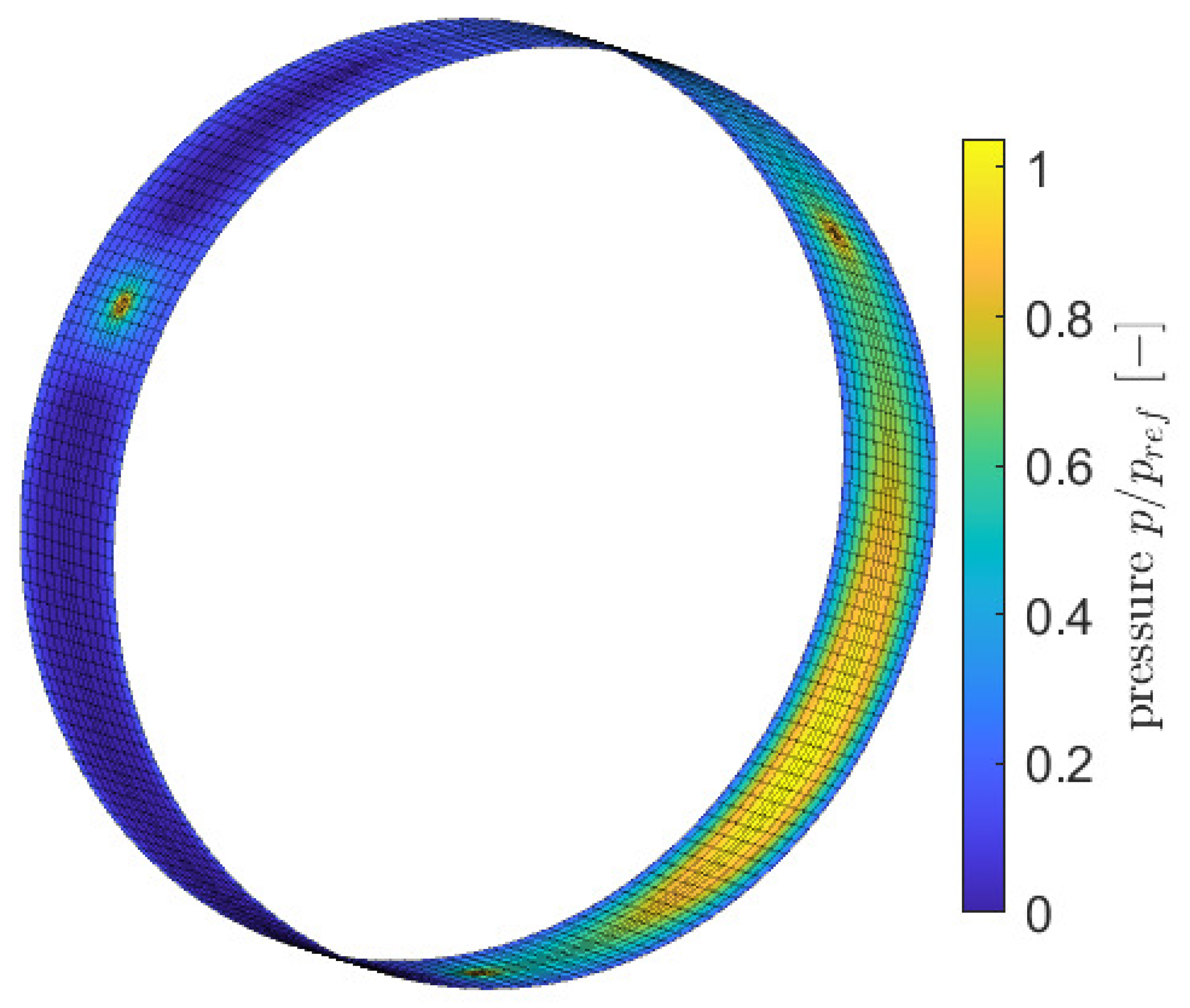
4. Results and Discussion
5. Conclusions
Author Contributions
Funding
Data Availability Statement
Acknowledgments
Conflicts of Interest
References
- Reynolds, O., IV. On the theory of lubrication and its application to Mr. Beauchamp tower’s experiments, including an experimental determination of the viscosity of olive oil. Philos. Trans. R. Soc. Lond. 1886, 177, 157–234. [Google Scholar]
- Dubois, G.B.; Ocvirk, F.W. The short bearing approximation for plain journal bearings. Trans. Am. Soc. Mech. Eng. 1955, 77, 1173–1178. [Google Scholar] [CrossRef]
- Yamamoto, T.; Ishida, Y. Rotordynamics: A Modern Treatment with Applications; Wiley: Hoboken, NJ, USA, 2001. [Google Scholar]
- Della Pietra, L.; Adiletta, G. The Squeeze Film Dampers over Four Decades of Investigations. Part I: Characteristics and Operating Features. Shock Vib. Dig. 2002, 34, 3–26. [Google Scholar]
- Hori, Y. Hydrodynamic Lubrication, 1st ed.; Springer: Tokyo, Japan, 2006. [Google Scholar] [CrossRef]
- Szeri, A.Z. Fluid Film Lubrication; Cambridge University Press: Cambridge, UK, 2010. [Google Scholar]
- Someya, T. Stabilität einer in zylindrischen Gleitlagern laufenden, unwuchtfreien Welle: Beitrag zur Theorie des instationär belasteten Gleitlagers. Ingenieur-Archiv 1963, 33, 85–108. [Google Scholar] [CrossRef]
- van Buuren, S. Modeling and Simulation of Porous Journal Bearings in Multibody Systems; KIT Scientific Publishing: Karlsruhe, Germany, 2014; Volume 21. [Google Scholar]
- Chatzisavvas, I. Efficient Thermohydrodynamic Radial and Thrust Bearing Modeling for Transient Rotor Simulations. Ph.D. Thesis, Technische Universität Darmstadt, Darmstadt, Germany, 2018. [Google Scholar]
- PW1100G-JM: Geared Turbofan Engine. Available online: https://www.mtu.de/engines/commercial-aircraft-engines/narrowbody-and-regional-jets/gtf-engine-family/ (accessed on 13 May 2024).
- Dowson, D.; Taylor, C. Cavitation in bearings. Annu. Rev. Fluid Mech. 1979, 11, 35–65. [Google Scholar] [CrossRef]
- Kumar, A.; Booker, J. A Finite Element Cavitation Algorithm: Application/Validation. J. Tribol. 1991, 113, 255–260. [Google Scholar] [CrossRef]
- Dowson, D. A generalized Reynolds equation for fluid-film lubrication. Int. J. Mech. Sci. 1962, 4, 159–170. [Google Scholar] [CrossRef]
- Pinkus, O.; Sternlicht, B.; Saibel, E. Theory of hydrodynamic lubrication. J. Appl. Mech. 1962, 29, 221–222. [Google Scholar] [CrossRef]
- Hamzehlouia, S.; Behdinan, K. Thermohydrodynamic Modeling of Squeeze Film Dampers in High-Speed Turbomachinery. SAE Int. J. Fuels Lubr. 2018, 11, 129–146. [Google Scholar] [CrossRef]
- San Andrés, L.; Vance, J.M. Effects of Fluid Inertia and Turbulence on the Force Coefficients for Squeeze Film Dampers. J. Eng. Gas Turbines Power 1986, 108, 332–339. [Google Scholar] [CrossRef]
- San Andrés, L.; Vance, J.M. Effects of Fluid Inertia on Finite-Length Squeeze-Film Dampers. ASLE Trans. 1987, 30, 384–393. [Google Scholar] [CrossRef]
- Hamzehlouia, S. Squeeze Film Dampers in High-Speed Turbomachinery: Fluid Inertia Effects, Rotordynamics, and Thermohydrodynamics. Ph.D. Thesis, Mechanical and Industrial Engineering, University of Toronto, Toronto, ON, Canada, 2017. [Google Scholar]
- Hamzehlouia, S.; Behdinan, K. A study of lubricant inertia effects for squeeze film dampers incorporated into high-speed turbomachinery. Lubricants 2017, 5, 43. [Google Scholar] [CrossRef]
- San Andrés, L. Force coefficients for a large clearance open ends squeeze film damper with a central feed groove: Experiments and predictions. Tribol. Int. 2014, 71, 17–25. [Google Scholar] [CrossRef]
- San Andrés, L.; Jeung, S.H.; Den, S.; Savela, G. Squeeze Film Dampers: An Experimental Appraisal of Their Dynamic Performance. In Proceedings of the First Asia Turbomachinery and Pump Symposium, Singapore, 22–25 February 2016. [Google Scholar]
- San Andrés, L.; Koo, B.; Jeung, S.H. Experimental Force Coefficients for Two Sealed Ends Squeeze Film Dampers (Piston Rings and O-Rings): An Assessment of Their Similarities and Differences. J. Eng. Gas Turbines Power 2018, 141, 021024. [Google Scholar] [CrossRef]
- Chatzisavvas, I.; Arsenyev, I.; Grahnert, R. Design and optimization of squirrel cage geometries in aircraft engines toward robust whole engine dynamics. Appl. Comput. Mech. 2023, 17, 93–104. [Google Scholar] [CrossRef]
- Lang, O.R.; Steinhilper, W. Gleitlager: Berechnung und Konstruktion von Gleitlagern Mit Konstanter und Zeitlich Veränderlicher Belastung; Springer: Berlin/Heidelberg, Germany, 1978. [Google Scholar]
- Rienäcker, A. Instationäre Elastohydrodynamik von Gleitlagern Mit Rauhen Oberflächen und Inverse Bestimmung der Warmkonturen. Ph.D. Thesis, RWTH Aachen, Aachen, Germany, 1995. [Google Scholar]
- San Andrés, L.; Delgado, A. A Novel Bulk-Flow Model for Improved Predictions of Force Coefficients in Grooved Oil Seals Operating Eccentrically. J. Eng. Gas Turbines Power 2012, 134, 052509. [Google Scholar] [CrossRef]
- Schmidt, M.; Reinke, P.; Rabanizada, A.; Umbach, S.; Rienäcker, A.; Branciforti, D.; Philipp, U.; Preuß, A.C.; Pryymak, K.; Matz, G. Numerical Study of the Three-Dimensional Oil Flow Inside a Wrist Pin Journal. Tribol. Trans. 2020, 63, 415–424. [Google Scholar] [CrossRef]
- Reinke, P.; Schmidt, M. Lokale, Hochauflösende 3D-CFD-Simulation der Schmierspaltströmung in Einem Instationär Belasteten Radialgleitlager; Final Report, No. 1154, FVV e.V.; FVV: Frankfurt/M, Germany, 2014; Volume 1073. [Google Scholar]
- Kistner, B. Modellierung und Numerische Simulation der Nachlaufstruktur von Turbomaschinen am Beispiel einer Axialturbinenstufe. Ph.D. Thesis, Technische Universität Darmstadt, Darmstadt, Germany, 1999. [Google Scholar]
- Khonsari, M.M.; Booser, E.R. Applied Tribology: Bearing Design and Lubrication; John Wiley & Sons, Ltd.: Hoboken, NJ, USA, 2017. [Google Scholar]
- Jaitner, D. Effiziente Finite-Elemente-Lösung der Energiegleichung zur Thermischen Berechnung Tribologischer Kontakte. Ph.D. Thesis, University of Kassel, Kassel, Germany, 2017. [Google Scholar]
- Hughes, T.J.; Tezduyar, T. Finite element methods for first-order hyperbolic systems with particular emphasis on the compressible Euler equations. Comput. Methods Appl. Mech. Eng. 1984, 45, 217–284. [Google Scholar] [CrossRef]
- Brooks, A.N. A Petrov-Galerkin Finite Element Formulation for Convection Dominated Flows. Ph.D. Thesis, California Institute of Technology, Pasadena, CA, USA, 1981. [Google Scholar]
- Codina, R. A discontinuity-capturing crosswind-dissipation for the finite element solution of the convection-diffusion equation. Comput. Methods Appl. Mech. Eng. 1993, 110, 325–342. [Google Scholar] [CrossRef]


| Measured [−] | Simulation [−] | Rel. Deviation |
|---|---|---|
Disclaimer/Publisher’s Note: The statements, opinions and data contained in all publications are solely those of the individual author(s) and contributor(s) and not of MDPI and/or the editor(s). MDPI and/or the editor(s) disclaim responsibility for any injury to people or property resulting from any ideas, methods, instructions or products referred to in the content. |
© 2024 by the authors. Licensee MDPI, Basel, Switzerland. This article is an open access article distributed under the terms and conditions of the Creative Commons Attribution (CC BY) license (https://creativecommons.org/licenses/by/4.0/).
Share and Cite
Golek, M.; Gleichner, J.; Chatzisavvas, I.; Kohlmann, L.; Schmidt, M.; Reinke, P.; Rienäcker, A. Numerical Simulations and Experimental Validation of Squeeze Film Dampers for Aircraft Jet Engines. Lubricants 2024, 12, 253. https://doi.org/10.3390/lubricants12070253
Golek M, Gleichner J, Chatzisavvas I, Kohlmann L, Schmidt M, Reinke P, Rienäcker A. Numerical Simulations and Experimental Validation of Squeeze Film Dampers for Aircraft Jet Engines. Lubricants. 2024; 12(7):253. https://doi.org/10.3390/lubricants12070253
Chicago/Turabian StyleGolek, Markus, Jakob Gleichner, Ioannis Chatzisavvas, Lukas Kohlmann, Marcus Schmidt, Peter Reinke, and Adrian Rienäcker. 2024. "Numerical Simulations and Experimental Validation of Squeeze Film Dampers for Aircraft Jet Engines" Lubricants 12, no. 7: 253. https://doi.org/10.3390/lubricants12070253