Abstract
Pavement texture and skid resistance are pivotal surface features of roadway to traffic safety, especially under wet weather. Engineering interventions should be scheduled periodically to restore these features as they deteriorate over time under traffic polishing. While many studies have investigated the effects of traffic polishing on pavement texture and skid resistance through laboratory experiments, the absence of real-world traffic and environmental factors in these studies may limit the generalization of their findings. This study addresses this research gap by conducting a comprehensive field study of pavement texture and skid resistance under traffic polishing in the real world. A total of thirty pairs of pavement texture and friction data were systematically collected from three distinct locations with different levels of traffic polishing (middle, right wheel path, and edge) along an asphalt pavement in Oklahoma, USA. Data acquisition utilized a laser imaging device to reconstruct 0.01 mm 3D images to characterize pavement texture and a Dynamic Friction Tester to evaluate pavement friction at different speeds. Twenty 3D areal parameters were calculated on whole images, macrotexture images, and microtexture images to investigate the effects of traffic polishing on pavement texture from different perspectives. Then, texture parameters and testing speeds were combined to develop friction prediction models via linear and nonlinear methodologies. The results indicate that Random Forest models with identified inputs achieved excellent performance for non-contact friction evaluation. Last, the friction decrease rate was discussed to estimate the timing of future maintenance to restore skid resistance. This study provides more insights into how engineers should plan maintenance to restore pavement texture and friction considering real-world traffic polishing.
1. Introduction
Skid resistance is an essential pavement property that measures the grip between pavement and tire, which is required for vehicle controllability. Possessing and maintaining appropriate skid resistance in pavement are essential for traffic safety, especially in wet weather, as this helps vehicles remain controllable [1,2,3]. Indeed, several empirical studies have shown the relationship between skid resistance and traffic safety (in terms of crashes). For example, in their field study in Texas, USA, McCullough and Hankins found that a large proportion of crashes were associated with low pavement skid resistance [4]. Similarly, Kuttesch found that the wet accident rate increases as road pavement skid resistance decreases [5]. It is thus far imperative to accurately measure and monitor the evolution of pavement skid resistance under traffic over time to understand its variation and schedule timely maintenance for restoration.
1.1. Pavement Texture and Traffic Polishing
According to [6], adhesion and hysteresis are two major components that contribute to pavement skid resistance. These two factors are greatly influenced by pavement surface texture, which is commonly classified into two categories, i.e., macro-, and microtextures. In ASTM 867-06 [7], macrotexture is defined as the surface with the characteristic dimensions of wavelength and amplitude from 0.5 mm up to those that no longer affect tire-pavement interaction (50 mm), and microtexture is defined as the surface with the characteristic dimensions of wavelength and amplitude less than 0.5 mm. These two types of textures affect the friction force developed at the contact zone between tire and pavement (i.e., skid resistance) in different ways. Previous studies have shown that pavement macrotexture provides drainage channels when it rains and comprises the hysteretic component of friction [8,9]. On the other hand, pavement microtexture was considered to provide actual contact with the tire and comprise the adhesion part of friction [10]. How these two different textures contacting vehicle tires seems to affect friction force at different vehicle traveling speeds. Macrotexture was found to provide a large proportion of friction force when a vehicle is driving above 56 mph (90 km/h) on wet pavements, while microtexture was found to have more impact on friction during low speed [2].
However, pavement texture does not remain intact after use, and pavement is subject to traffic-induced wear or traffic polishing [11,12,13,14,15]. To understand how bad the pavement texture is polished over time, which degraded skid resistance as a result, researchers and practitioners have looked at ways to profile both macro- and microtextures of pavement surface. The most common measurements of pavement macrotextures are the mean texture depth (MTD) and the mean profile depth (MPD). The MTD calculates the average depth of macrotexture determined by the sand patch method [16], and the MPD calculates the average of all mean segment depths of all the segments of the profile and is typically measured by laser-scan-based methods [17].
Albeit commonly adopted, the relationship between MPD and friction under traffic polishing is still undetermined. For example, Pomoni et al. [18] found negative correlation between MPD and the Mean Summer Skid Coefficient (MSSC). This is contradictory to what Kouchaki et al. [19] found in their study, where a positive correlation was found between MPD and grip number (GN, another friction measurement index). Pomoni et al. [18] provided possible explanations of other factors (e.g., textural components) that may contribute to the phenomenon (i.e., the contradictory relationship between MPD and skid resistance). The undetermined relationship between MPD and friction has advocated further research on the topic and to explore other ways (e.g., indexes and devices) to better understand some determinants of surface texture that reduce skid resistance after traffic polishing.
On the other hand, pavement microtexture is considered the most affected texture class under traffic polishing as it is the highest part that is in contact with vehicle tires [20]. For microtexture profiling, it is commonly measured using devices such as the British Portable Tester (BPT) and the Dynamic Friction Tester (DFT) at lower speed [21]. Despite the effort that has been carried out by previous studies, researchers have not come to a consensus for the profiling methods.
Nowadays, with the advancement of technology and higher sensor resolution, it is possible to capture both macro- and microtextures at the same time using a laser-based scanner or optical sensors. Laser-based scanners and optical sensors also have the benefit of profiling surface textures with spatial parameters (e.g., power spectrum density of a rough surface), function parameters (e.g., areal material ratio) or hybrid parameters (e.g., root mean square gradient and interfacial area ratio) (see [22] for definitions and full list). In addition, using a single device to capture both macro- and microtextures allows a more time-saving texture profiling for monitoring the evolution of pavement under traffic polishing as equipment set up time could be reduced. For example, Zou et al. [15] conducted a field study and collected 3D areal parameters with a portable 3D laser scanner. Twenty parameters were derived from the 3D image over a 3-year data collection period. This study showed the feasibility of using 3D images to find what microtexture and macrotexture parameters deteriorated after traffic polishing on asphalt pavements.
1.2. Pavement Friction and Traffic Polishing
As mentioned previously, pavement textures are worn under traffic polishing. For asphalt pavements, after the overlying film is worn away, it is likely the deterioration of pavement friction occurs subsequently with traffic continually passing by [18]. Pavement friction is the resistance to motion between vehicle tires and pavement surfaces and this resistance force is also called skid resistance. Monitoring skid resistance evolution over time is necessary if it deteriorates to the level that vehicle tires do not have a good grip on the surface pavement, as this can increase the risk of skidding-related hazards.
Skid resistance is commonly measured with BPT and DFT in lab or performed on site for spot inspection and represented as the British Pendulum Number (BPN) and dynamic friction coefficients, respectively. Another common measurement in the lab environment of skid resistance is the Polished Stone Value (PSV), an indicator that reflects the ability of coarse aggregate to maintain certain levels of friction against tire abrasion which is typically collected through comparison of specimens with and without undergoing repeated tire loads. A growing trend in recent years is to utilize the Wehner/Schulze device for pavement aggregate or surface layers to facilitate the study of the correlation of skid resistance between measurements taken in lab and in the field [23].
With the capability to profile surface texture and measure friction level, there have been interests in developing skid resistance evolution modelling in hopes of providing an accurate prediction of timing of surface pavement maintenance to retain appropriate skid resistance level after traffic polishing. For example, Rezaei et al. [24] conducted lab experiments with different design mixtures of aggregates. After different polishing cycles, an international friction index predictive function was developed based on aggregate characteristics and gradation. Li et al. [25] developed statistical models with survival analysis which not only identified important factors to skid resistance (e.g., roadway curvature) but also provided a tool that for pavement maintenance decision making. A more recent work by Kane et al. [26] on modelling collected surface texture data from 3D topographies to predict skid resistance after traffic polishing, a dynamic friction model was incorporated and increased the overall model performance.
The models are a convenient way to predict maintenance needs; however, models were typically built under certain data collection environment, and thus not always being suitable to be generalized. Some researchers have also argued that in-lab tests may not fully represent skid resistance evolution due to other influencing factors like weather, traffic loading, and geometric features of a roadway [25], and thus continuous skid resistance monitoring in the field is still a reliable way to evaluate skid resistance and are sometimes suggested to reflect the real polishing status. Some commonly used devices for high-speed friction measurement on the field are locked-wheel testers [27], continuous friction measurement equipment (CFME, [28]), the GripTester system for a unitless friction measurement Grip Number (GN, [29]), and the Side force Coefficient Routine Investigatory Machine (SCRIM, [27]).
The phenomenon of skid resistance decrease after traffic polishing was found in multiple previous studies as empirical evidence showing that traffic polishing decreases surface pavement friction in addition to the change in pavement texture. Meegoda and Gao [30] conducted correlation analysis between skid resistance (skid numbers) and macrotexture. It was found that at different MPD values, correlation directions with skid resistance level were different, and traffic polishing factor needs to be considered for older surface pavements. Specifically, the polishing of macrotexture seems to incur an insufficiency of pavement drainage, which increases the water in the tire/road contact area and results in the decrease of skid resistance [31]. On the other hand, some empirical studies have shown microtexture to be a more important pavement characteristic that directly impacts skid resistance [18,31], and it may have a positive relationship according to a correlation analysis by Wang et al. [32].
Several traffic characteristics have been taken into account as well when investigating the relationship between traffic polishing and pavement friction. For example, Chu et al. [12] collected BPNs at different pavement sections under both wheel path and non-wheel path, and different vehicle operation modes (e.g., acceleration, deceleration, and cruising). Their results showed significant effects of traffic polishing and vehicle operation modes on pavement skid resistance. In addition, traffic composition is another factor affecting the extent to which the surface is polished. For instance, Khasawneh et al. [33] considered the count of heavy vehicles as an predictor in their regression model and found it to be a significant factor in the model for predicting macrotexture level, which has an indication of change in skid resistance. Plati and Pomoni [34] were interested in knowing how traffic volumes affect pavement macrotexture and skid resistance over time in the field, and they found that unlike lab study, trend of macrotexture and skid resistance were not always similar under traffic polishing. A minimum cumulative traffic threshold is reached before we can see an opposite trend (negative correlation) between skid resistance and macrotexture. More importantly, heavy traffic volume seems to be a more important factor than traffic volume overall in influencing macrotexture and skid resistance, which is in accordance with what [33] found.
The findings that various traffic characteristics contribute to skid resistance deterioration support the importance of conducting field investigations under real traffic and climate conditions through long-term monitoring. In addition, the fact that [34] found an unsimilar trend between macrotexture and skid resistance, and reminded it may not be appropriate to develop a long-term prediction model for skid resistance based on early-life pavement data urges more research to be performed. A holistic approach that considers pavement texture and friction simultaneously after traffic polishing needs to be further explored to minimize time-consuming resource-intensive field long-term monitoring.
1.3. Objectives
At present, there is an existing body of studies focused on laboratory evaluation of simulated traffic polishing on pavement texture and friction. As alluded earlier, lab studies may not capture the full picture of how real-world traffic impacts pavement texture and friction over time given that there may be other factors in the actual driving environment amplifying the change in texture and friction such as climate conditions. On the other hand, when studies move to the field, some previous studies focused on the impact of traffic polishing on either pavement texture or friction only. If pavement texture and friction are collected in the field simultaneously, the data will be inherently suitable to explore the relationship between texture and friction under the impact of real-world traffic polishing.
Additionally, the pavement friction decrease rate over time has typically been investigated through laboratory experiments or long-term field studies, both of which are time-consuming and resource-intensive. Across the horizontal direction of a roadway, distinct areas undergo varying degrees of traffic polishing over time: the roadway wheel path experiences the highest level of traffic polishing, followed by the middle areas and edges of the roadway. Therefore, friction numbers across roadway horizontal direction could represent the trend of pavement friction deterioration under traffic polishing over time: the roadway wheel path could have the lowest friction numbers due to the highest level of traffic polishing, followed by higher friction numbers at roadway middle areas and edges due to less traffic polishing. Accordingly, monitoring friction numbers along roadway horizontal direction could lead to an efficient alternative to calculate the pavement friction decrease rate without laboratory experiments or long-term field studies.
To address the research gap mentioned above, the current study aims to perform a holistic investigation of the impact of traffic polishing on pavement texture and friction simultaneously in the field. More specifically, pavement 3D texture images and friction data were collected via a laser imaging system and a DFT from an asphalt pavement after seven years of service. The obtained 0.01 3D texture images were visually inspected to understand how traffic polishing affects whole images, macrotexture images, and microtexture images. Afterwards, computation of 20 distinct 3D areal parameters, spanning height, spatial, hybrid, functional, and feature parameters, was conducted to explore the effects of traffic polishing on pavement texture from diverse perspectives. Following this, texture parameters and testing speeds were combined to develop friction prediction models via linear and nonlinear methodologies for non-contact friction evaluation. Lastly, the friction decrease rate was discussed via considering the assumed accumulated traffic polishing and friction numbers along roadway horizontal directions to estimate the timing of future maintenance for skid resistance restoration.
2. Field Data Collection
This section presents the details of field data collection via two devices on an asphalt pavement. With traffic control, this study collected pavement texture and friction data on two field sections from the Country Club Road in Stillwater, Oklahoma, USA, in 2022. The roadway was constructed with asphalt concrete (AC) using an asphalt binder of PG 70–28 and an aggregate combination of 23% 3/4″ Chips + 28% Mine Chat + 15% Man. Sand + 19% Scrns + 14% Sand + 1% B.H.Fines. Per Table 1, the laboratory testing result showed that the aggregate and asphalt mixture used on that AC roadway had good performance to meet the agency’s requirements. In addition, the gradation of the S4 mixture used on that AC roadway satisfied the agency’s gradation requirements, as shown in Figure 1.

Table 1.
Summary of laboratory testing results of AC.
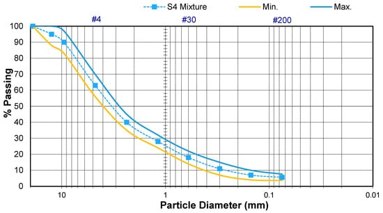
Figure 1.
Gradation Curves for Aggregate Combinations.
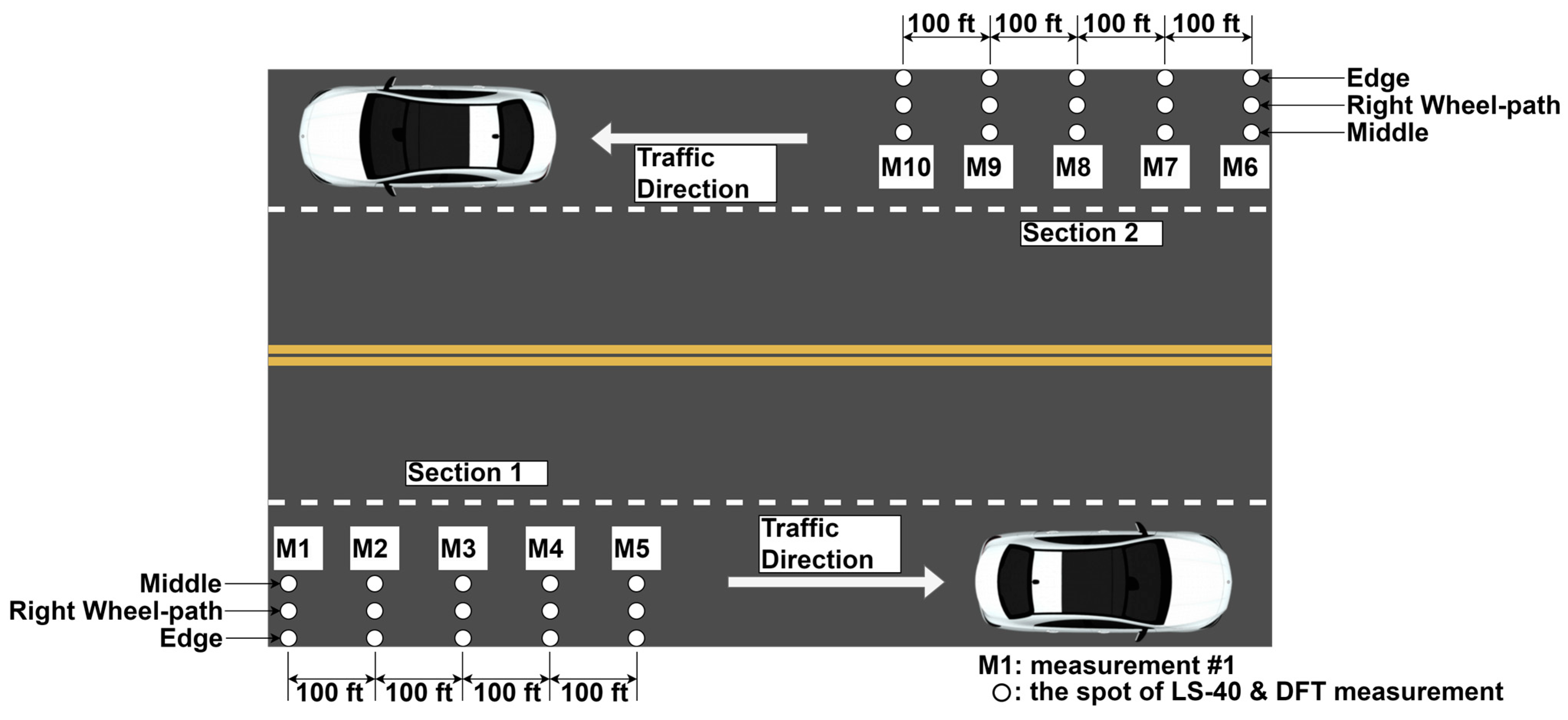
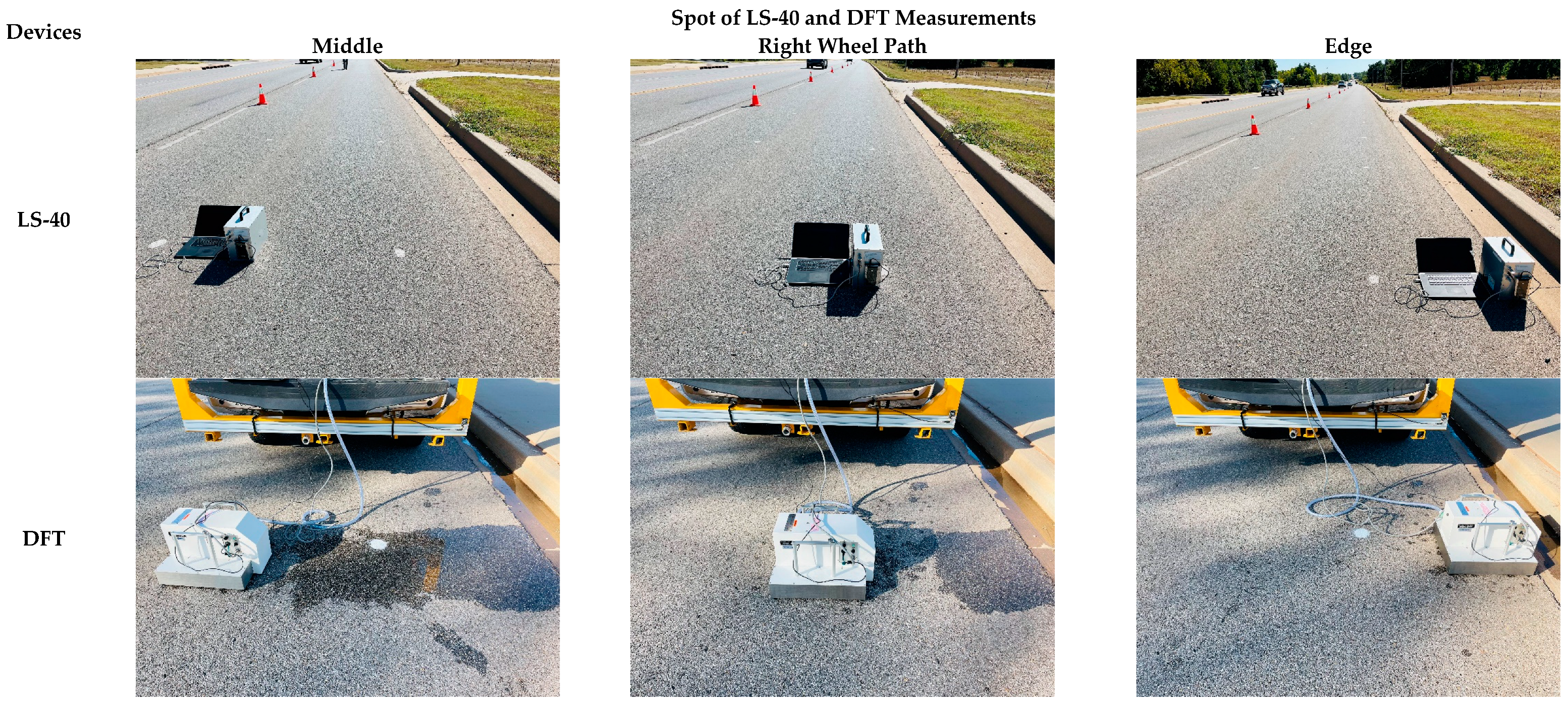
As shown in Figure 2, a total of 30 pairs of pavement texture and friction data were systematically collected from two sections along three distinct locations with different levels of traffic polishing: the middle, right wheel path, and edge of the outer travel lane. In each section, measurements for texture and friction were taken at five locations, each spaced 30.5 m (100 feet) apart. Figure 3 displays images of devices utilized for field data collection on the three locations: a 3D laser imaging device, LS-40, which reconstructs 3D images with a resolution of 0.01 mm to characterize pavement texture; and a DFT, employed to evaluate pavement friction at varying speeds (10–70 km/h).
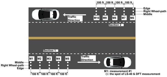
Figure 2.
Location scheme of field data collection along the roadway.
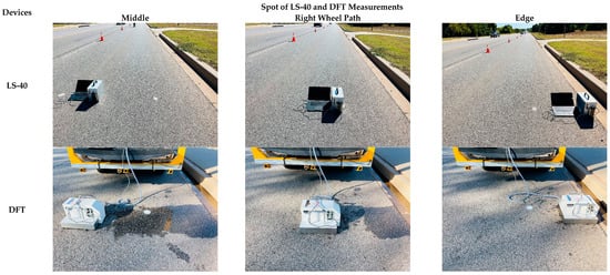
Figure 3.
Field pavement texture and friction measurements via LS-40 and DFT.
It is reasonable to assume that the right wheel path experienced the most traffic polishing, followed by the middle and edge of the outer travel lane. Consequently, the pavement texture and friction data gathered from distinct locations on the road, including the middle, right wheel path, and edge, will enable us to discern how varying levels of traffic polishing impact pavement surface characteristics. For instance, we anticipate that the right wheel path, experiencing the highest level of traffic polishing, may exhibit smoother surface textures and lower friction coefficients compared to those from the less-polished middle and edge of the travel lane.
3. Pavement Texture Evaluation
As shown in Figure 2, each measurement collected data from three locations that are within the same travel lane. Because these locations are close to each other, it is reasonable to assume that climate factors (e.g., temperature, wind, precipitation, sunshine, etc.) have had the same impact on the pavement texture characteristics over the past few years. Therefore, any changes in pavement texture at these locations are likely due to varying levels of traffic polishing happened as vehicles passing by. For instance, most vehicles move along wheel path under normal forward driving conditions, which leads to extensive polishing on pavement texture within wheel path area. Accordingly, the 0.01 mm 3D pavement images obtained from the middle, right wheel path, and edge of the outer travel lane during field data collection provide ideal data source to investigate how pavement texture varies under real traffic and environment impacts.
To characterize pavement texture variations under traffic polishing, the collected 0.01 mm 3D texture images from the middle, right wheel path, and edge of the outer travel lane were virtually compared first. Then, these images were denoised and separated as macro- and microtexture images to visually inspect if traffic polishing impact differently on pavement macro- or microtextures. Afterwards, 3D areal parameters of denoised whole images, macrotexture images, and microtexture images will be calculated and compared to investigate how traffic polishing affects pavement texture characteristics at different locations. Details of pavement texture characteristics under traffic polishing are summarized and discussed as follows.
3.1. Texture Characteristics via Vision Observation
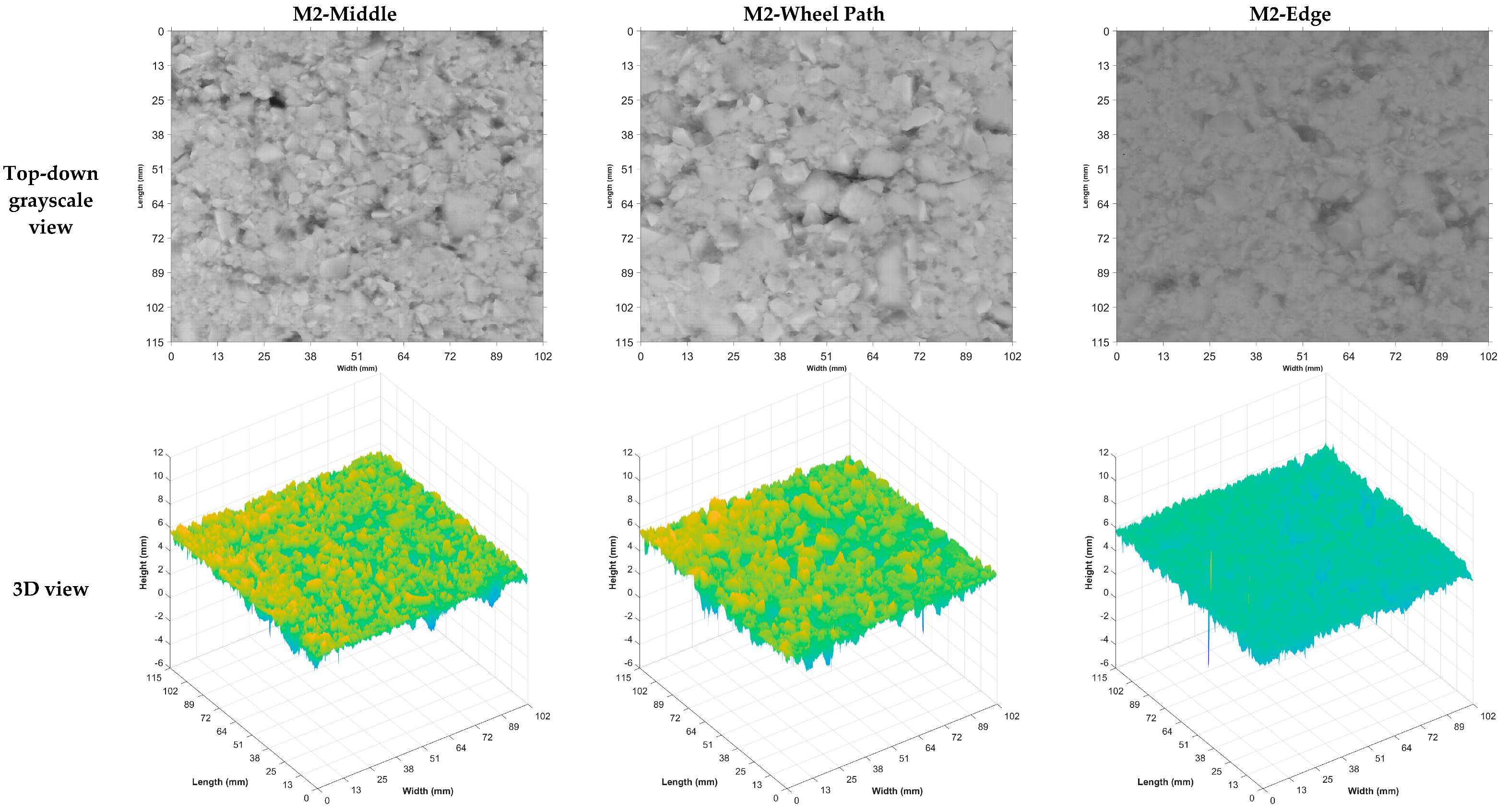
In this section, pavement texture characteristics under traffic polishing are evaluated visually via comparing original images, denoised images, macrotexture images, and microtexture images from LS-40 at different locations. As shown in Figure 4, using measurement #2 as an example, original 0.01 mm 3D pavement images from the middle, right wheel path, and edge of the outer travel lane exhibits different texture characteristics after experiencing seven years of traffic polishing:
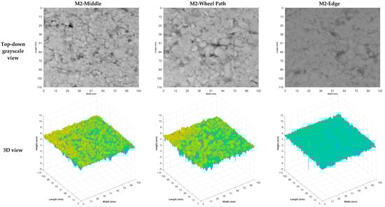
Figure 4.
Original 3D pavement texture data from LS-40.
- (1)
- Many large aggregates are exposed in the top-down grayscale image from wheel path due to extensive traffic polishing in the last seven years.
- (2)
- The top-down grayscale image from the middle of the travel lane shows a mix of large, medium, and small size aggregates after experiencing certain traffic polishing over seven years of service.
- (3)
- The top-down grayscale image from the edge of the travel lane exhibits only a few aggregates due to minimal traffic polishing after seven years of service.
- (4)
- The 3D view of these images demonstrates a similar trend of the number of exposed aggregates from these locations. However, the original images should be processed to remove the noise for further analysis.
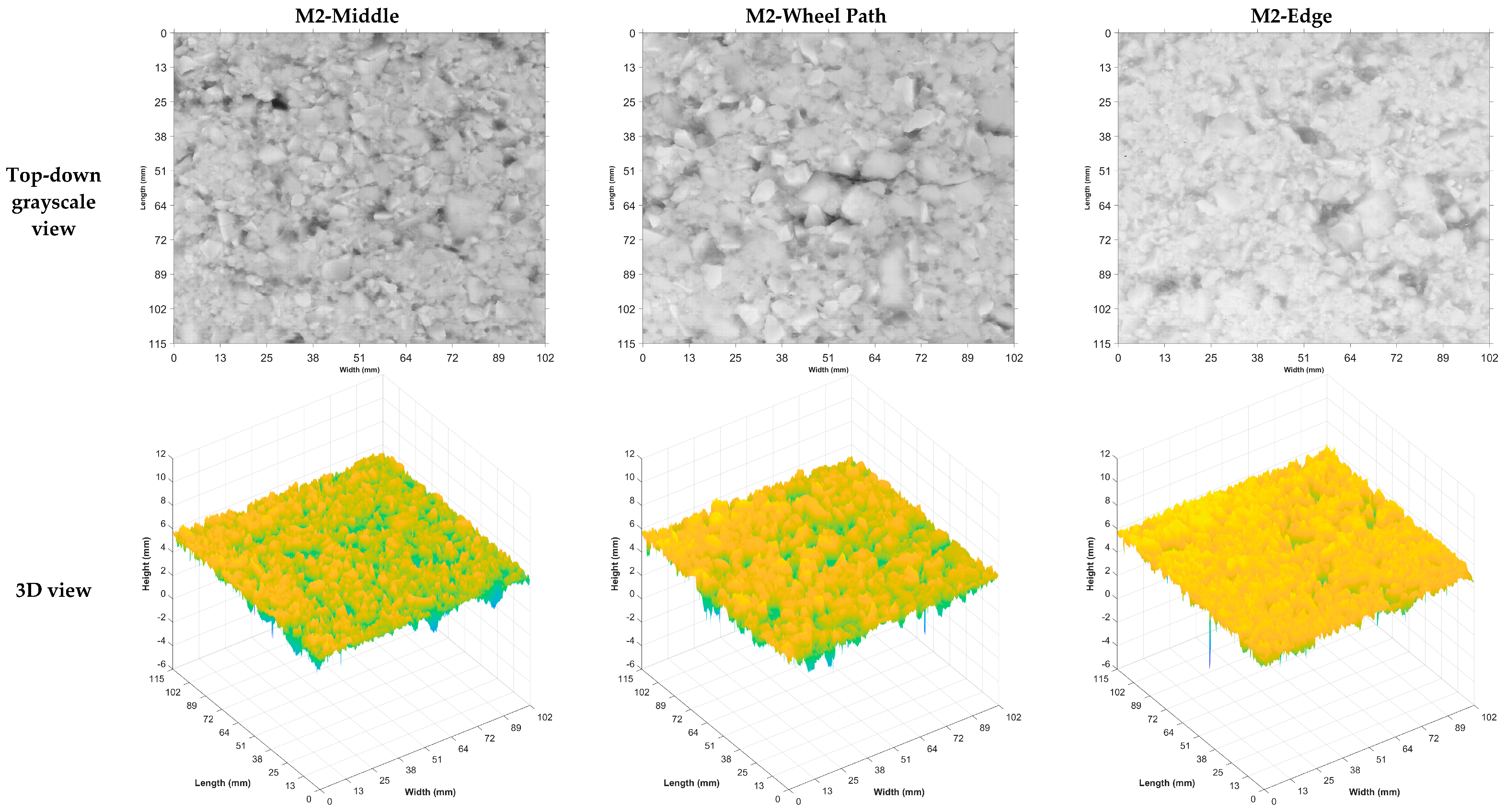
To denoise the 0.01 mm 3D images, the cumulative distribution of the height values of these images was analyzed. It was found that 98% of the height values was within 6.419 mm and the average height values was 5.149 mm. Therefore, any pixels with height values larger than 6.419 mm will be treated as noise and replaced with a random height value between 5.149 mm and 6.419 mm. Pixels with height values less than or equal to 6.419 mm will be retained to represent the original texture characteristics captured by the LS-40. Figure 5 shows the denoised 3D pavement texture data from LS-40 in top-down grayscale view and 3D view. Particularly, when comparing Figure 4 and Figure 5, the denoised images (top-down grayscale view or 3D view) from the edge of the travel lane better display texture distribution. It indicates that the simple denoise method was effective in removing noise while retaining original texture characteristics. The denoised images in Figure 5 more clearly depict a higher presence of large aggregates exposed in the wheel path location, followed by those in the middle and edge of the travel lane due to different levels of traffic polishing over time.

Figure 5.
Denoised 3D pavement texture data from LS-40.
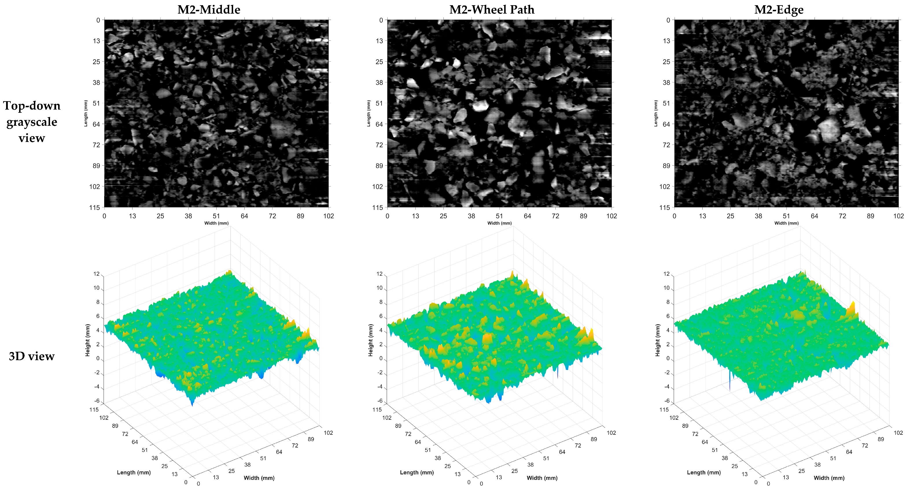
Because the 3D images from LS-40 have a resolution of 0.01 mm, it provides an opportunity to investigate how traffic polishing affects pavement texture at different scales, e.g., macro- or microtextures. To accomplish this, the Butterworth filter was applied on the denoised whole images to obtain (1) macrotextures with a wavelength between 0.5 mm and 50 mm and (2) microtextures with a wavelength less than 0.5 mm. Figure 6 and Figure 7 illustrate pavement macro- and microtexture images obtained from Butterworth filter.

Figure 6.
3D pavement macrotexture data from LS-40.
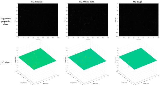
Figure 7.
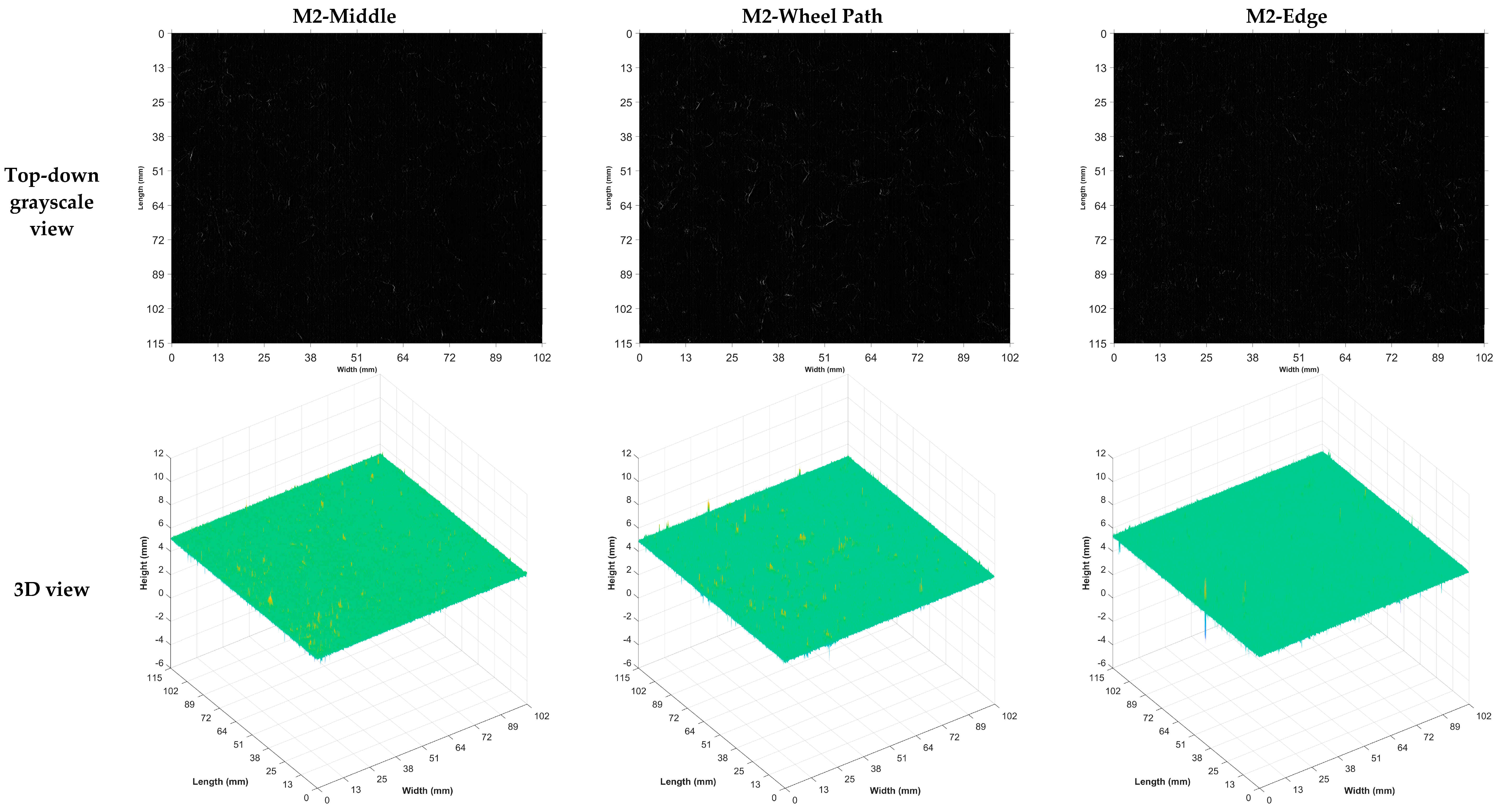
3D pavement microtexture data from LS-40.
In Figure 6, the macrotexture images in top-down grayscale view and 3D view distinctly reveal that many aggregates are exposed in the image of wheel path due to extensive traffic polishing, followed by the image of middle of the travel lane and the image of edge of the travel lane. In the 3D view images in Figure 7, spikes are evident in the microtexture of the wheel path, with fewer spikes seen in the images of the middle and edge of the travel lane. This is because the wheel path as more valleys and variations in texture height along the valleys produce high-frequency information or low-wavelength textures, which are filtered out as spikes in the microtexture images. However, these spikes have small height values (less than 2 mm) while many other non-spike pixels of the microtexture images have height values close to zero. In grayscale images, pixel values close to zero are displayed as black, while pixel values close to 1 (or 255, depending on the bit depth) are displayed as white. Therefore, the microtextures images in the top-down grayscale view in Figure 7 are mostly black, with minor bright spots corresponding to the small spikes observed in the 3D view.
3.2. Texture Characteristics via 3D Areal Parameters
In this section, 3D areal parameters of denoised whole images, macrotexture images, and microtexture images from the middle, right wheel path, and edge of the outer travel lane were calculated and compared to investigate how traffic polishing affects pavement texture characteristics from different perspectives. Specifically, 20 different 3D areal texture parameters were calculated on those 0.01 mm 3D images across the following five categories [15]:
- (1)
- Three height parameters: arithmetic mean height (Sa, unit: mm), root mean square height (Sq, unit: mm), skewness (Ssk without unit), and kurtosis (Sku without unit),
- (2)
- Three spatial parameters: autocorrelation length (Sal, unit: mm), texture aspect ratio (Str without unit), and texture direction (Std, unit: rad),
- (3)
- Two hybrid parameters: root mean square gradient (Sdq without unit) and developed interfacial area ratio (Sdr, unit: %),
- (4)
- Nine functional parameters: peak extreme height (Sxp, unit: mm), surface section difference (Sdc, unit: mm), reduced peak height (Spk, unit: mm), core height (Sk, unit: mm), reduced dale height (Svk, unit: mm), peak material volume (Vmp, unit: mm3), core material volume (Vmc, unit: mm3), core void volume (Vvc, unit: mm3), and dales void volume (Vvv, unit: mm3),
- (5)
- Three feature parameters: peak density (Spd, unit: mm−2) and peak curvature (Spc, unit: mm−1).
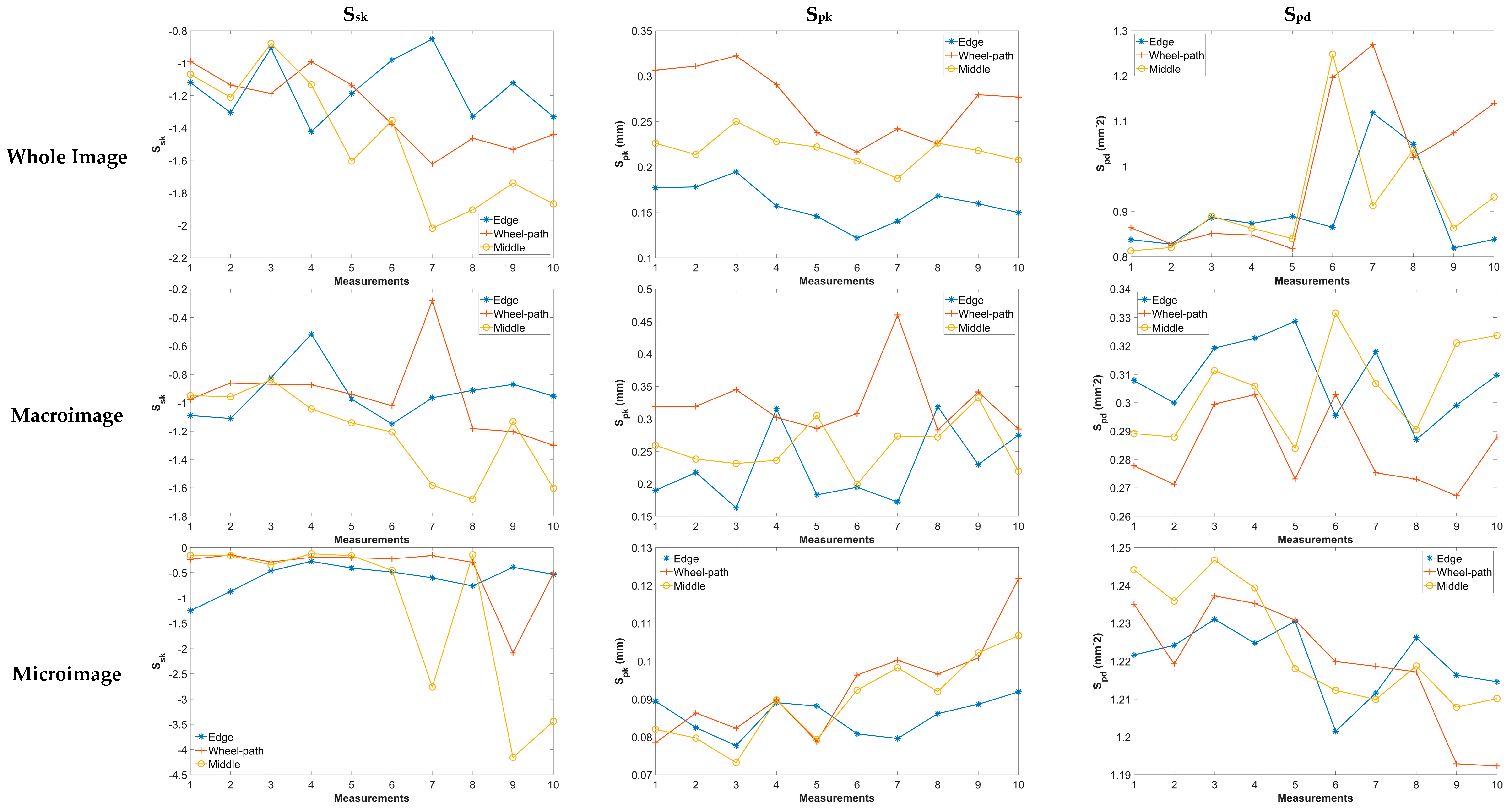
Due to length limitations, it is challenging to present all the results of the twenty texture parameters of these whole images, macrotexture images, and microtexture images herein. Accordingly, the Ssk, Spk, and Spd are discussed in detail, as they are selected as critical texture parameters for friction prediction via Random Forest models, which will be covered in Section 4.2. Specifically, the Ssk will be negative if pavement surface has valley structure, the Spk represents the primary and most worn texture height, and a large Spd indicates the surface has more points of contact with other object [15].
Figure 8 shows the original distribution of Ssk, Spk, and Spd of whole images, macrotexture images, and microtexture images from the middle, right wheel path, and edge of the outer travel lane for all measurements. The Spk of whole images is the only parameter that shows clear difference under traffic polishing: the wheel path shows the highest Spk, followed by those from the middle and edge of the travel lane. It means that pavement aggregates in the wheel path area are mostly exposed after extensive traffic polishing, resulting in higher or more prominent peaks above the core roughness profile. In contrast, the smaller Spk of whole images from the middle and edge of the travel lane suggest that the aggregates in these areas are not fully exposed yet due to less traffic polishing. Observing the other texture parameters in Figure 8, it is challenging to distinguish how traffic polishing affects pavement texture for the middle, right wheel path, and edge of the outer travel lane, regardless of whether they were calculated from whole images, macrotexture images, or microtexture images.
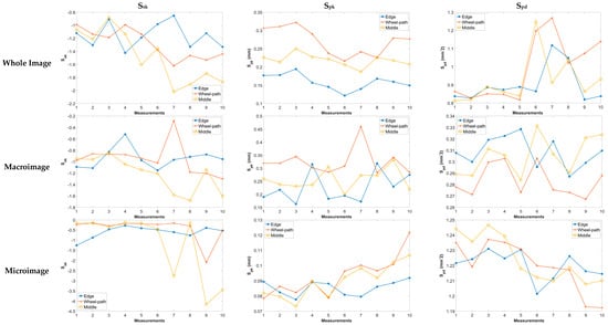
Figure 8.
Example texture parameters of whole, macro-, and microimages from all measurements.
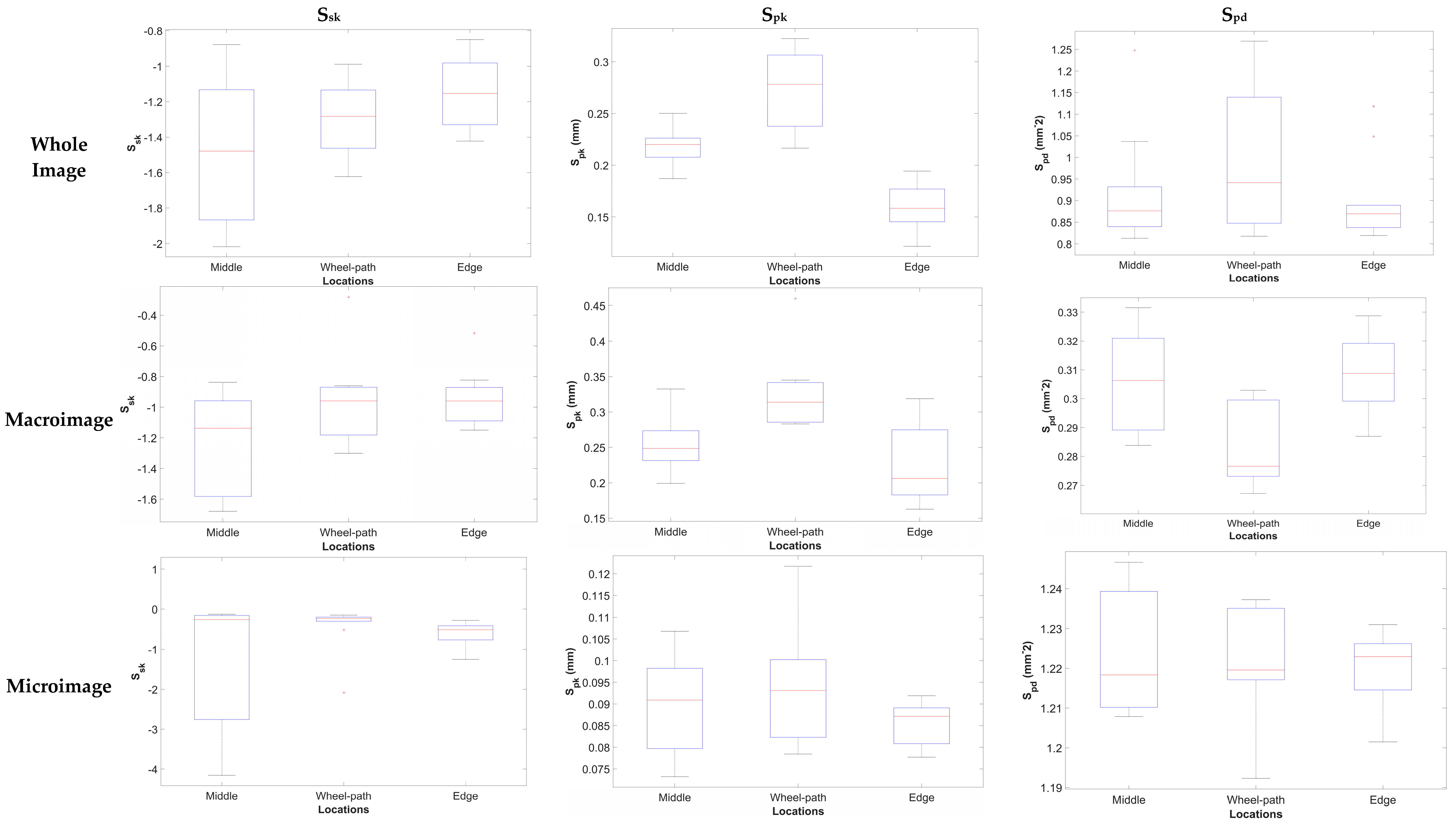
Then, Figure 9 shows the maximum, average, and minimum distribution of Ssk, Spk, and Spd of whole images, macrotexture images, and microtexture images from the middle, right wheel path, and edge of the outer travel lane for all measurements. A few conclusions can be drawn to explain how different levels of traffic polishing affect these 3D areal parameters:
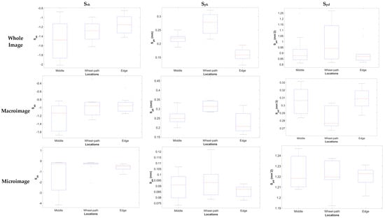
Figure 9.
Summary of texture parameters of whole, macro-, and microimages from all measurements.
- (1)
- For Ssk, all of them are negative numbers for whole images, macrotexture images, and microtexture images, which means the height distribution of pavement texture is skewed below the mean plane, suggesting all these textures have more low points or depressions compared to high points or peaks due to traffic polishing. For whole images, the edge shows an average Ssk of −1.15 while the middle shows an average Ssk of −1.48. It indicates that the edge texture has a less pronounced negative skew. In other words, the edge surface has fewer valleys or is less asymmetric than the middle texture due to less aggregates exposed under less traffic polishing. A similar trend is observed in the Ssk of macrotexture images. For microtexture images, all Ssk are negative but close to zero, indicating the microtexture still has more low points than high points, but with less difference between the wheel path, middle, and edge of the roadway.
- (2)
- For all three image categories, the wheel path shows a higher average Spk, which is followed by those from the middle and edge of roadway. Generally, a larger Spk indicates that the surface has higher or more prominent peaks above the core roughness profile [15]. It means that as traffic polishing accumulated on pavement surface, the Spk of whole images, macrotexture images, or microtexture images increases, signifying more aggregates are exposed on the surface as higher or prominent peaks above the core roughness profile. However, the Spk of microtexture are less than those of whole images or macrotexture images, and not showing significant difference among the three locations, as shown in Figure 9.
- (3)
- The whole images and microtexture images have larger Spd than macrotexture images. The whole image exhibits a higher Spd due to the presence of all surface protrusions, while microtexture images capture fine protrusions and filtering artifacts, resulting in higher Spd than macrotexture images. Also, from whole images, a larger average Spk is observed on wheel path, followed by middle and edge of the roadway. This suggests that traffic polishing generates more peaks per unit texture area on roadway, even though it wears down pavement texture and aggregates are exposed over time. For macrotexture images, the average Spk for wheel path, middle, and edge of roadway is close to each other with little variations and around 0.3 because the peaks or spikes in macrotexture images (Figure 6) are not as many as shown in whole images (Figure 5) or microtexture images (Figure 7).
Accordingly, these 3D areal texture parameters are effective to characterize pavement texture development due to traffic polishing over time. By leveraging these parameters, we can develop accurate friction prediction models for non-contact pavement skid resistance evaluation, which will be presented in chapter 4. This approach could minimize the need for traditional friction testing devices that require testing tires or water [27,29], thereby streamlining the pavement friction evaluation process and enhancing efficiency.
4. Pavement Friction Evaluation
This section presents the DFT numbers of these measurements from the middle, right wheel path, and edge of the outer travel lane to characterize how field pavement friction evolves under varying levels of real traffic polishing and environment impact over time. Then, the previously calculated 3D areal texture parameters and the DFT testing speeds (10–70 km/h) will be combined as training dataset to develop friction prediction models via various methodologies (Random Forest, neural network, and stepwise multivariate linear regression). The best friction prediction model will be selected from various models with different inputs and training methodologies for future non-contact friction evaluation via 3D texture parameters.
4.1. Friction Characteristics Under Traffic Polish
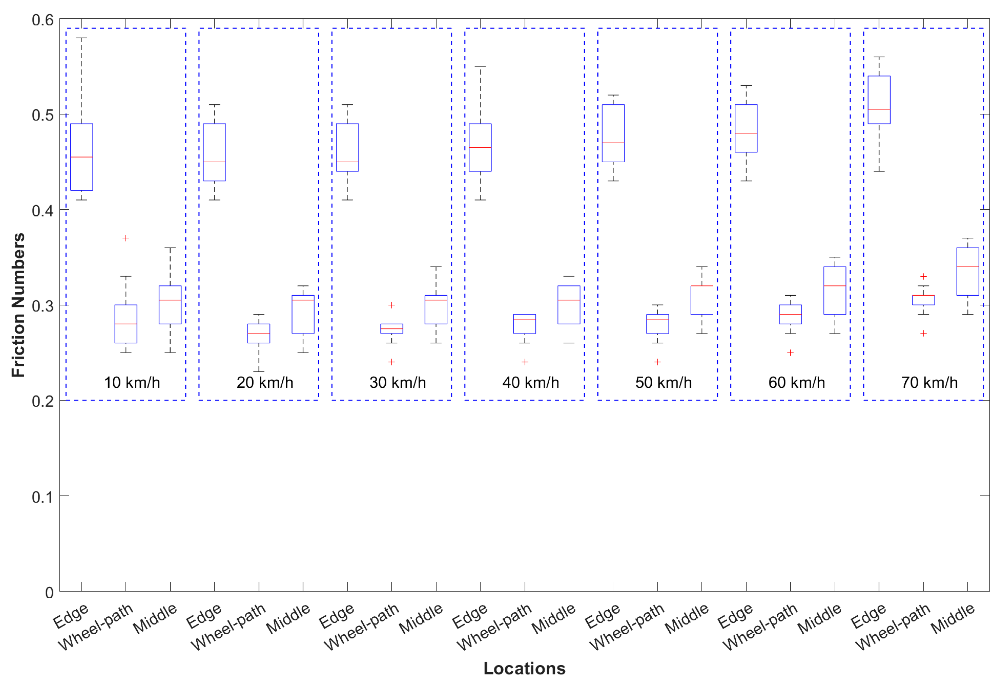
During DFT testing, when rotating speed achieves the target speed, the spinning disk with three testing rubber sliders will drop off and gradually stop spinning due to pavement skid resistance. Therefore, the DFT is able to measure and save pavement friction numbers from testing speeds of 10–70 km/h. Figure 10 displays the maximum, average, and minimum distribution of DFT numbers for testing speed of 10–70 km/h from the middle, right wheel path, and edge of the outer travel lane. A few conclusions can be drawn to explain how different levels of traffic polishing affect pavement friction:
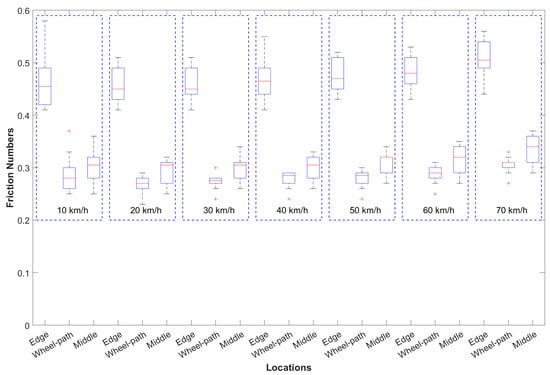
Figure 10.
Distribution of friction numbers from different locations at various testing speeds.
- (1)
- Under each testing speed, the edge of the outer travel lane shows the highest average friction number, followed by those from the middle and right wheel path due to traffic polishing. For example, at speed of 60 km/h, the average friction numbers are 0.48, 0.32, and 0.29, separately, for the edge, middle, and right wheel path of the outer travel lane. It indicates that pavement areas under extensive traffic polishing (wheel path) shows lower skid resistance than pavement areas experiencing less traffic polishing (middle or edge).
- (2)
- Furthermore, the collected DFT numbers exhibit slight increase as testing speeds changed from 10–70 km/h, as shown in Figure 10. This phenomenon could be due to the testing speed not being high enough to cause a decrease for this particular asphalt mixture. Nevertheless, it still indicates that testing speed affects the collected friction numbers via DFT even though the pavement texture is not changed. So, testing speed should be considered as one input when developing pavement friction prediction models via 3D areal texture parameters.
- (3)
- All DFT measurements were completed in approximately 60 min under traffic control, with an ambient temperature of 75 °F. Consequently, the temperature influence on these DFT numbers will be ignored, as they were collected under consistent ambient conditions. Thus, temperature will not be considered as an input when developing pavement friction prediction models.
Therefore, the DFT measurements from the middle, right wheel path, and edge of the outer travel lane captured pavement friction variations due to different levels of traffic polishing over time. These DFT numbers will be utilized in the next section to develop pavement friction prediction models via 3D areal texture parameters and DFT testing speeds. Further, combining the variations in pavement friction numbers and the number of traffic polishing, the friction decrease rate could be estimated (as presented in chapter 5) for recommending future maintenance to restore pavement skid resistance and minimize friction related crash risks.
4.2. Friction Prediction Models
Many efforts have been implemented to develop friction prediction models to (1) investigate the relationship between pavement texture and friction and (2) achieve non-contact pavement friction evaluation without consuming tire or water. For instance, Kováč et al. developed friction models to predict BPT numbers via 3D texture parameters using multivariate linear regression model [35]. Koné applied machine learning models to predict pavement friction coefficient from speed, MPD, water depth, and tire tread depth [36]. Yang et al. proposed a conventional neural network (CNN) model to predict pavement GN numbers via two-dimensional texture profiles obtained from various field sites [37]. Lu et al. also presented a CNN model for friction prediction via texture features and identified textures with wavelengths above 2.4 mm is key for wet BPT numbers [38]. However, these studies were not using texture parameters from the same asphalt mixture but after different levels of traffic polishing for developing friction prediction models.
To investigate how texture parameters correlate to friction numbers under different levels of traffic polishing, this section presents the development of friction prediction models via three methodologies based on 3D areal texture parameters and DFT testing speeds. As shown in Figure 2, a total of 30 pairs of LS-40 and DFT data were systematically collected from the middle, right wheel path, and edge of the outer travel lane with different levels of traffic polishing. Then, 20 different 3D areal texture parameters were calculated for each of the 0.01 3D images to characterize texture properties from five perspectives, including height parameters, spatial parameters, hybrid parameters, functional parameters, and feature parameters. Further, a total of 210 DFT numbers from eight different speeds ranging from 10 to 70 km/h, as illustrated in Figure 10, were considered when developing friction prediction models. Finally, two sets of inputs were prepared as follows to investigate whether texture parameters from whole images or macro-/microtexture images are more important when developing accurate friction prediction models:
- (1)
- Input 1: a matrix with a dimension of 21 (20 areal parameters from whole images and one testing speed) by 210 (a total of 210 samples to match 210 DFT numbers across seven different speeds);
- (2)
- Input 2: a matrix with a dimension of 41 (20 areal parameters from macrotexture images, 20 areal parameters from microtexture images, and one testing speed) by 210 (a total of 210 samples to match 210 DFT numbers across seven different speeds).
For each input, 70% of the prepared data was used for model training and the remaining 30% was kept for model testing. Furthermore, Random Forest (RF) [39], neural network (NN) [40,41], and stepwise multivariate linear regression (SMLR) [42] were selected to develop friction prediction models for the following reasons: (1) these methodologies were successfully applied to develop friction prediction models in previous studies, (2) the number of dataset in this study was not enough to explore deep learning models, and (3) these methods investigated if there is a linear (SMLR) or a nonlinear (RF and NN) relationship between pavement texture parameters and friction numbers.
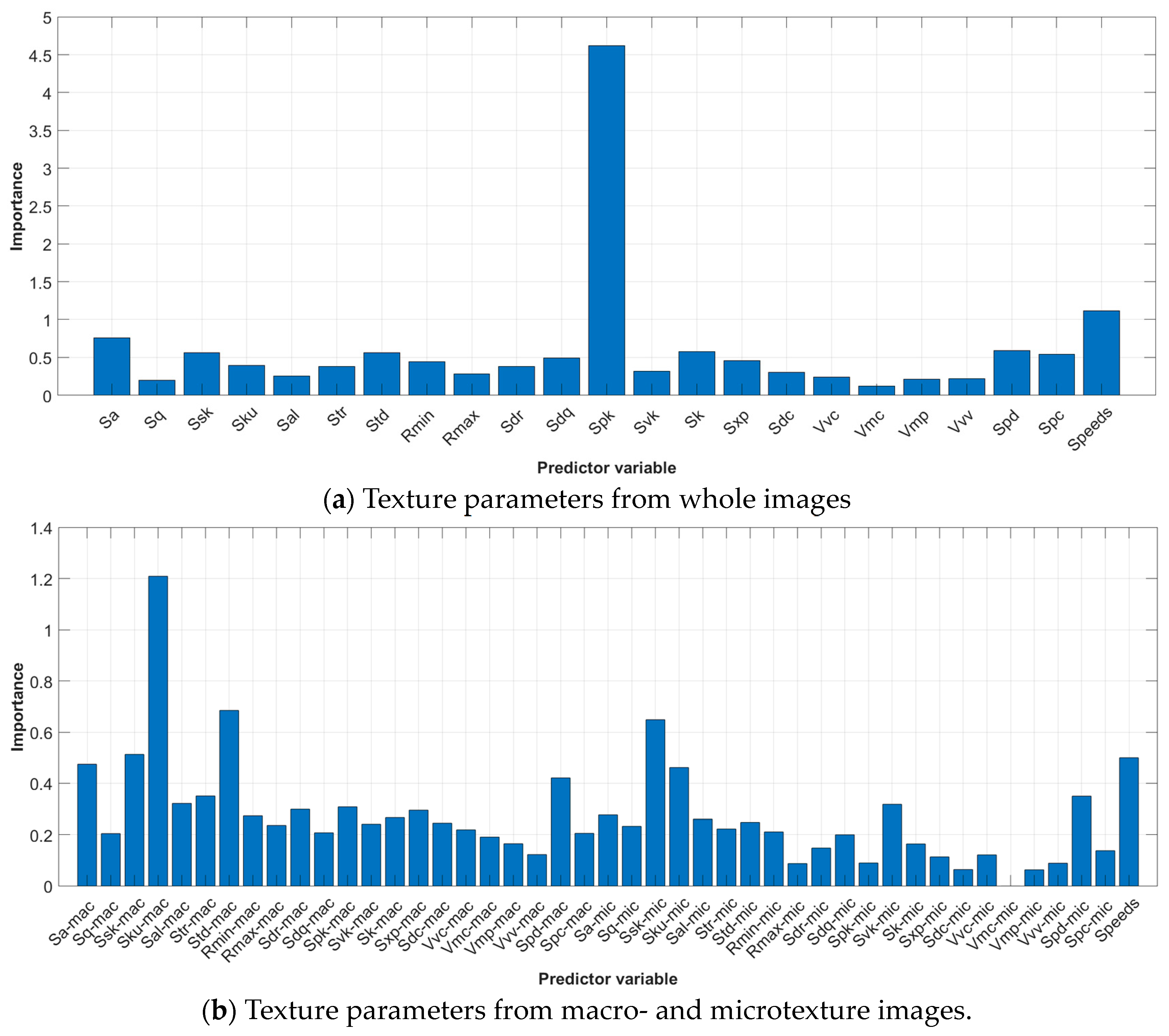
Particularly, for RF models, six different numbers of trees (50, 100, 150, 200, 250, and 300) were considered during model development to select the best model. Additionally, each RF model used all predictor variables at each node to ensure that every tree utilized all predictors. The importance of each input was estimated by permuting out-of-bag observations among the trees to select the critical texture parameters for friction prediction via RF models, as shown in Figure 11. Finally, variables with importance larger than 0.5 were selected to develop the RF models. For instance, as shown in Figure 11a, Sa, Ssk, Std, Spk, Sk, Spd, and Spc from whole images and speeds are selected as critical texture parameters for friction prediction when using Input 1.
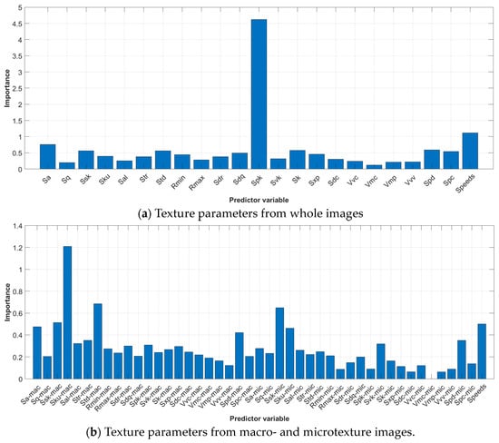
Figure 11.
Importance estimation for selecting critical parameters for friction prediction via RF models. (a) Sa, Ssk, Std, Spk, Sk, Spd, and Spc from whole images and speeds are selected as critical parameters for friction prediction. (b) Ssk-mac, Sku-mac, Std-mac from macrotexture images, Ssk-mic from microtexture images, and speeds are selected as critical parameters for friction prediction.
For NN model, it had a network with two hidden layers, each consisting of 20 units. Also, it used the Scaled Conjugate Gradient algorithm as the training algorithm to explore the nonlinear relationship between input (pavement texture parameters and testing speed) and output (friction numbers). All the parameters were involved in NN training while 90% and 10% of the training data were used for model training and validation.
For SMLR, it created a linear model for the friction numbers using stepwise regression to add or remove predictors (pavement texture parameters and testing speed). The 0.05 was selected as the threshold for the criterion to add or remove a variable to the model. In other words, a variable will be selected if its corresponding p-values is less than 0.05, and vice versa. Consequently, the final SMLR model contains only the selected parameters deemed important for friction prediction.
Further, during model training, 10-fold cross-validation was applied to generalize the model’s performance. The training data were randomly divided into 10 equal subsamples, with nine used for training and one for validation. This process was repeated 10 times, each time using a different subsample for validation. The model’s general performance was estimated by averaging the R-squared values from all 10 iterations, a commonly used metric for assessing a model’s goodness of fit.
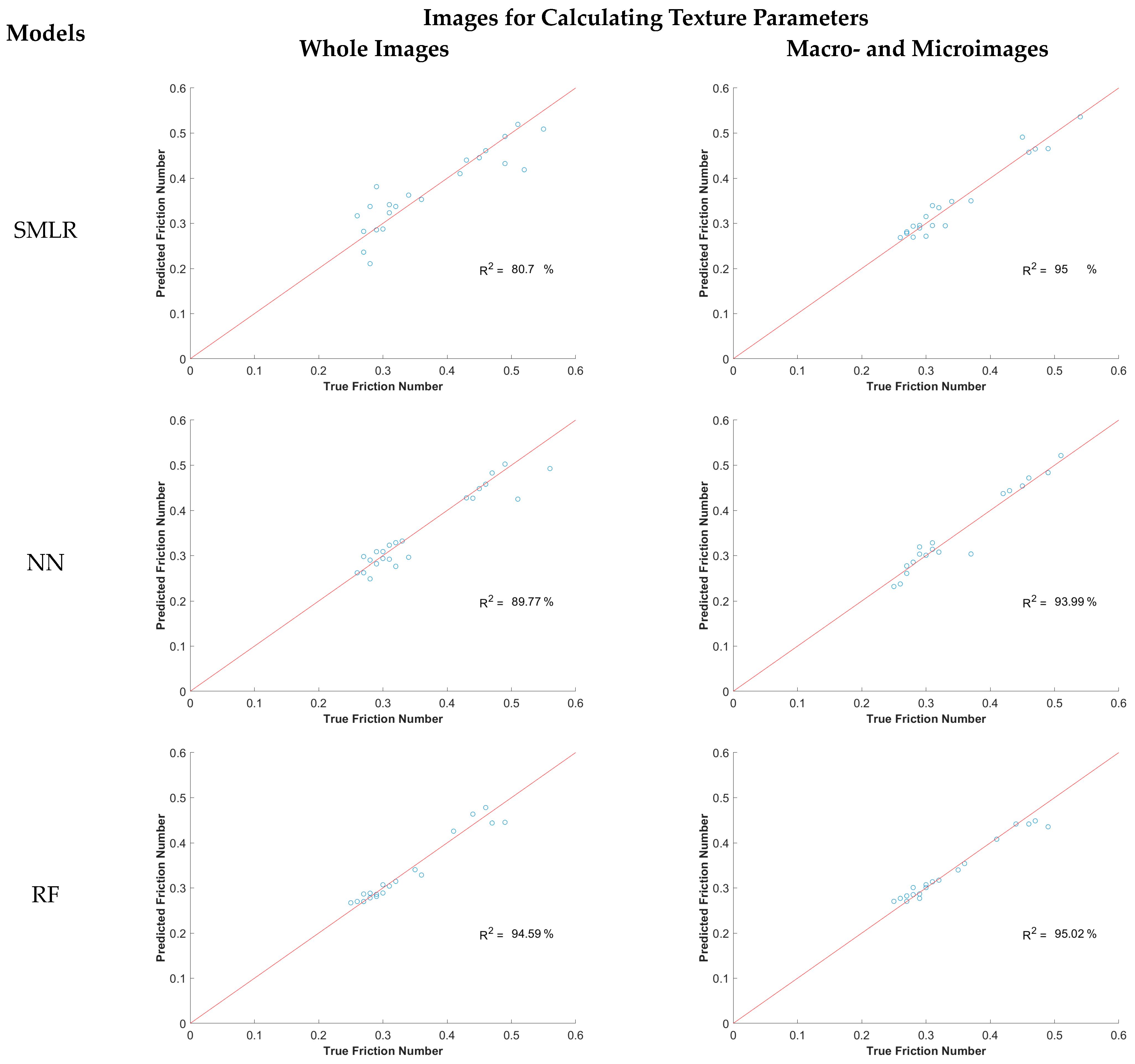
Therefore, the R-squared values of the best friction prediction models via Input 1 and Input 2 are listed in Table 2. Specifically, Ssk, Spk, Spd, and speeds are the selected parameters in SMLR when using whole images, while Sku-mac, Str-mac, Std-mac, Rmin-mac, Str-mac, Sdq-mac, Sk-mac, Sxp-mac, Vmc-mac, Spd-mac, and Spc-mac from macrotexture images, Rmax-mic and Spc-mic from microtexture images, and speeds are the most selected parameters in SMLR when using macro-/microtexture images. Also, Sa, Ssk, Std, Spk, Sk, Spd, and Spc from whole images and speeds are the selected parameters in RF with 100 trees when using whole images, while Ssk-mac, Sku-mac, Std-mac from macrotexture images, Ssk-mic from microtexture images, and speeds are the selected parameters in RF with 250 trees when using macro-/microtexture images. Further, Figure 12 shows the testing examples of the SMLR, NN, and RF models from 10 cross-validations using the prepared testing data from Input 1 and Input 2.
Table 2.
Summary of R-squared values of the best friction prediction models.
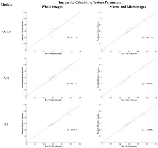
Figure 12.
Testing examples of the best friction prediction models from 10 cross-validations.
Table 2 and Figure 12 offer insights into characterizing the relationship between pavement texture parameters and friction numbers as follows:
- (a)
- A nonlinear relationship exists between pavement texture parameters and friction numbers. This is evidenced by the lower R-squared values of the SMLR model compared to those of the NN or RF models, regardless of whether whole images or macro-/microtexture images were used to calculate 3D areal texture parameters.
- (b)
- Reduced peak height (Spk) emerges as the critical texture parameter in developing friction prediction models, as evidenced by both the SMLR and RF always selecting Spk as the critical input.
- (c)
- Friction models using 3D texture parameters from macro-/microtexture images outperformed those using texture parameters from whole images. For instance, the NN model reached an R-squared value of 89.52% with whole image parameters, but 94.29% when using 3D macro-/microtexture parameters. It indicates that separating whole images into macro-/microlevels for parameter calculation benefits the accuracy of friction prediction models.
- (d)
- Testing speed should be considered when developing friction prediction models.
Finally, the best RF model via 3D texture parameters from macro-microtexture images achieved an R-squared value of 94.63% when comparing the predicted friction numbers against the true friction numbers on the testing data. It indicates that the proposed RF model can perform non-contact friction evaluation with excellent accuracy based on the selected inputs (Ssk-mac, Sku-mac, Std-mac from macrotexture images, Ssk-mic from microtexture images, and speeds). Accordingly, the high-resolution 3D images from LS-40 provide an ideal alternative to (1) investigate the impact of traffic polishing on pavement texture and friction, and (2) conduct non-contact friction evaluation using the proposed model, thereby potentially minimizing the need for traditional friction testing devices that require testing tires or water.
5. Discussion of the Friction Decrease Rate
This section discusses the friction decrease rate by examining the assumed cumulative traffic polishing and friction numbers across roadway horizontal directions, aiming to estimate the timing for future maintenance to restore skid resistance. The speed limit of the roadway was 45 mph, while the average daily traffic (ADT) for the two sections was 3031 and 3107, individually, as calculated per Table 3, with 80% traffic being two axles’ cars. To estimate the accumulated traffic along the edge, wheel path, and middle of the two testing sections, three engineering assumptions were developed as follows:
Table 3.
Summary of average daily traffic (ADT) on testing sites.
- (1)
- The traffic growth rate on this roadway is 2%.
- (2)
- 50% of the vehicles travel along the right travel lane, as shown in Figure 2.
- (3)
- There are 1%, 80%, and 19% traffic polishing happening along the edge, wheel path, and middle of the roadway for these two testing sites. It means (a) minimal vehicles (1%) move to roadway edge due to wandering or uncommon maneuvers, (b) most vehicles (80%) move along roadway wheel path under normal forward driving, and (c) certain vehicles (19%) move and polish roadway middle area due to vehicle wandering, lane change, or other maneuvers.
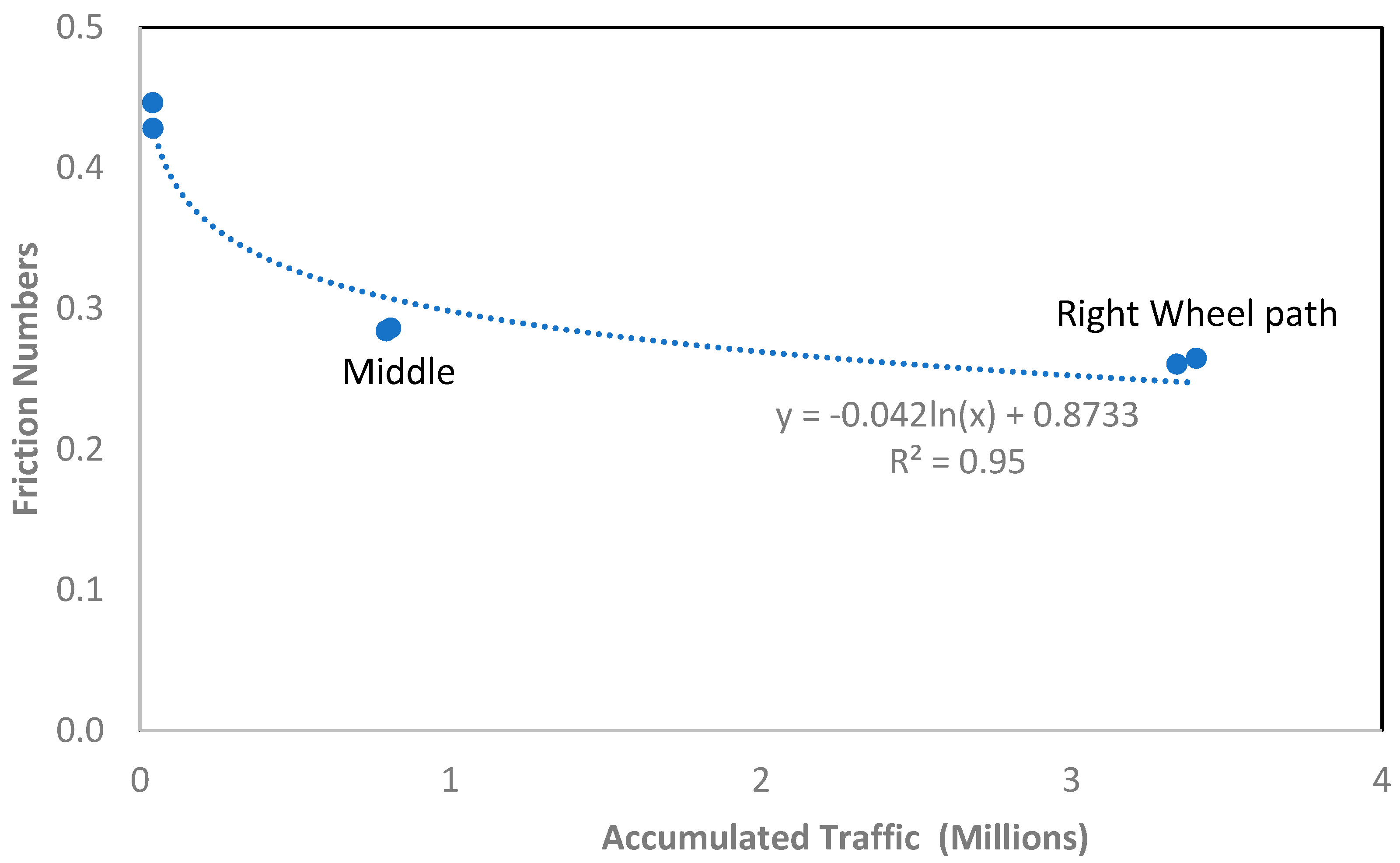
Accordingly, from 2015 to 2022, the accumulated traffic is estimated as 4.13 million on Section 1 and 4.23 million on Section 2. Then, per assumption (3), the accumulated traffic along the edge, wheel path, and middle of the two testing sections are estimated and listed in Table 4. Figure 13 shows the logarithmic relationship between pavement friction numbers and accumulated traffic along roadway edge, wheel path, and middle areas, achieving an R-squared value of 0.95. Figure 13 presents a slower friction decrease rate as traffic accumulated on the pavement. Furthermore, it means that friction numbers along roadway horizontal direction (edge, middle, wheel path, etc.) could represent different stages of the evolvement of pavement skid resistance under various levels of traffic polishing and environmental impact in the field.
Table 4.
Summary of average friction numbers and accumulated traffic at different locations from the two testing sections.
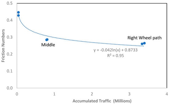
Figure 13.
Relationship between pavement friction numbers and accumulated traffic.
For example, the roadway edge experienced 1% of accumulated traffic polishing over seven years, which could represent the early stage of asphalt pavement with binder removed and oxidized but limited aggregates exposed after 0.42 million of traffic in seven years. The middle of roadway experienced approximately 0.80 million of traffic in seven years, so that pavement showed average friction numbers of approximately 0.28, which is less than 0.45 from the roadway edge but larger than 0.26 from the right wheel path because the aggregates underwent more polishing than the edge but less polishing than the right wheel path.
Furthermore, as traffic accumulated, the decrease rate of pavement friction slowed down, as observed from other studies via long term observations [8,28,43]. Therefore, comparing the data in Figure 13 for middle and wheel path, as the right wheel path went through more than 3 million of traffic polishing over seven years, its friction numbers was still 0.26. It means friction numbers of this roadway decreased only 0.02 on average after experiencing 2.5 million more traffic polishing when comparing the friction numbers and accumulated traffic at the middle and right wheel path of this roadway. This phenomenon aligns well with other studies that did laboratory investigations of pavement friction under different levels of polishing cycles [43,44,45]. However, to obtain the friction decrease rate for a longer term, the proposed framework, as shown in Figure 13, only measured friction numbers from roadway locations experiencing different levels of traffic polishing along pavement horizontal direction (e.g., middle, wheel path, and edge) without requiring performing extensive laboratory testing to polishing pavement samples or long-term field monitoring over time.
Therefore, the future pavement friction numbers on this roadway could be estimated per the projected accumulated traffic per Equation (1). For instance, when selecting friction numbers of 0.2 as maintenance threshold, the projected accumulated traffic per Figure 13 or Equation (1) will be 9.16 million on this road. It indicates the road would reach friction numbers of 0.2 by the year 2031 for potential maintenance, which is 16 years of service since its opening to the public in 2015 given the traffic condition and pavement mixture characteristics.
It is worth noting that the friction decrease rate herein was estimated per the given traffic conditions and roadway structures or mixtures only. Pavement constructed with other materials for varying traffic conditions would exhibit varying rates of friction decrease. However, the proposed framework demonstrates the possibility of predicting future pavement friction numbers via simply testing pavement friction numbers along horizontal directions (e.g., edge, wheel path, middle of roadway) and assumed accumulated traffic polishing. The proposed framework could minimize the need for laboratory testing to polish the samples or long-term friction monitoring, which could be affected by testing temperatures, locations, or speed over time.
6. Conclusions
This study presents a field investigation of pavement texture and skid resistance evolution under real-world traffic polishing via 0.01 mm 3D images. The pavement texture and friction data were collected via a laser image device and a DFT, individually, from the middle, right wheel path, and edge of an asphalt roadway in Oklahoma, USA. To characterize pavement texture variations under traffic polishing, the 3D images from various locations were processed as whole images, macrotexture images, and microtexture images for visually inspection and calculation of 20 different 3D areal texture parameters from five perspectives (height, spatial, hybrid, functional, and feature). The results indicate that the wheel path had extensive large aggregate exposure from significant traffic polishing over the last seven years, the middle of the lane showed a mix of aggregate sizes due to moderate polishing, and the edge displayed minimal aggregate exposure from limited polishing. The calculated 3D areal texture parameters were able to characterize these texture variations due to traffic polishing at whole image, macro- and microtexture levels.
Furthermore, the roadway edge showed the highest average friction number, followed by the middle and right wheel path under different DFT testing speeds, due to different levels of traffic polishing over time. The texture parameters were then combined with the DFT testing speed to develop friction prediction models via linear and nonlinear methodologies. The RF model achieved an excellent performance for friction prediction with the selected inputs (height parameters skewness (Ssk-mac) and kurtosis (Sku-mac), spatial parameter (Std-mac) from macrotexture images, height parameters skewness (Ssk-mic) from microtexture images, and DFT testing speed), indicating a nonlinear relationship between pavement texture parameters and friction numbers.
Last, the friction decrease rate was discussed based on the assumed accumulated traffic polishing and measured friction numbers along roadway horizontal directions (edge, middle, and wheel path). The proposed framework determines friction decrease rates via roadway friction numbers along horizontal direction under varying levels of traffic polishing, without requiring extensive laboratory testing or long-term field monitoring. It could offer an efficient method for estimating future maintenance timing to restore pavement skid resistance based on cumulative real-world traffic passes.
However, it is worth noting that the developed friction prediction models and friction decrease rate are developed based on the limited data collections in this study. A wide range of pavement sections with other texture and friction properties are desired in future research to improve their robustness and general performance. Also, the obtained friction decrease rate should be validated against long-term field monitoring data to verify its accuracy and effectiveness. Lastly, detailed traffic data (e.g., vehicle classes, percentage of trucks) should be included in future studies to improve the model’s performance as well.
Author Contributions
Conceptualization, G.Y.; methodology, G.Y.; software, G.Y. and Y.Z.; validation, G.Y.; formal analysis, G.Y.; investigation, G.Y.; resources, K.W. and J.L.; data curation, G.Y.; writing—original draft preparation, G.Y. and K.-T.C.; writing—review and editing, G.Y. and K.-T.C.; visualization, G.Y. All authors have read and agreed to the published version of the manuscript.
Funding
This research received no external funding.
Data Availability Statement
The raw data supporting the conclusions of this article will be made available by the corresponding author on request.
Conflicts of Interest
Author Yiwen Zou was employed by the company China Railway City Development and Investment Group, China Railway Group Limited. The remaining authors declare that the research was conducted in the absence of any commercial or financial relationships that could be construed as a potential conflict of interest.
References
- Ahammed, M.A.; Tighe, S.L. Asphalt Pavements Surface Texture and Skid Resistance—Exploring the Reality. Can. J. Civ. Eng. 2012, 39, 1–9. [Google Scholar] [CrossRef]
- Flintsch, G.W.; McGhee, K.K.; Najafi, S. The Little Book of Tire Pavement Friction. Pavement Surf. Prop. Consort. 2012, 1, 1–22. [Google Scholar]
- Transportation Research Board. Designing Safer Roads; Transportation Research Board: Washington, DC, USA, 1987. [Google Scholar]
- McCullough, B.F.; Hankins, K. Skid Resistance Guidelines for Surface Improvements on Texas Highways; Highway Research Record: Washington, DC, USA, 1966. [Google Scholar]
- Kuttesch, J. Quantifying the Relationship between Skid Resistance and Wet Weather Accidents for Virginia Data. Master’s Thesis, Virginia Polytechnic Institute and State University, Blacksburg, VA, USA, 2004. [Google Scholar]
- Cairney, P. Skid Resistance and Crashes—A Review of the Literature; Research Report/Australian Road Research Board; Australian Road Research Board: Vermont South, Australia, 1997; ISBN 978-0-86910-750-8. [Google Scholar]
- ASTM E867-06; Standard Terminology Relating to Vehicle-Pavement Systems. ASTM: West Conshohocken, PA, USA, 2020.
- National Academies of Sciences, Engineering and Medicine. Guide for Pavement Friction; The National Academies Press: Washington, DC, USA, 2009. [Google Scholar]
- Villani, M.M.; Artamendi, I.; Kane, M.; Scarpas, A. (Tom) Contribution of Hysteresis Component of Tire Rubber Friction on Stone Surfaces. Transp. Res. Rec. 2011, 2227, 153–162. [Google Scholar] [CrossRef]
- Forster, S.W. Pavement Microtexture and Its Relation to Skid Resistance. Transp. Res. Rec. 1989, 1215, 151–164. [Google Scholar]
- Chu, L.; Cui, X.; Zhang, K.; Fwa, T.F.; Han, S. Directional Skid Resistance Characteristics of Road Pavement: Implications for Friction Measurements by British Pendulum Tester and Dynamic Friction Tester. Transp. Res. Rec. 2019, 2673, 793–803. [Google Scholar] [CrossRef]
- Chu, L.; Zhou, B.; Fwa, T.F. Directional Characteristics of Traffic Polishing Effect on Pavement Skid Resistance. Int. J. Pavement Eng. 2022, 23, 2937–2953. [Google Scholar] [CrossRef]
- Do, M.-T.; Tang, Z.; Kane, M.; de Larrard, F. Pavement Polishing—Development of a Dedicated Laboratory Test and Its Correlation with Road Results. Wear 2007, 263, 36–42. [Google Scholar] [CrossRef]
- Do, M.-T.; Tang, Z.; Kane, M.; De Larrard, F. Evolution of Road-Surface Skid-Resistance and Texture Due to Polishing. Wear 2009, 266, 574–577. [Google Scholar] [CrossRef]
- Zou, Y.; Yang, G.; Huang, W.; Lu, Y.; Qiu, Y.; Wang, K.C.P. Study of Pavement Micro- and Macro-Texture Evolution Due to Traffic Polishing Using 3D Areal Parameters. Materials 2021, 14, 5769. [Google Scholar] [CrossRef]
- ASTM E965-15; Standard Test Method for Measuring Pavement Macrotexture Depth Using a Volumtric Technique. ASTM: West Conshohocken, PA, USA, 2019.
- ASTM E1845-01; Standard Practice for Calculating Pavement Macrotexture Mean Profile Depth. ASTM: West Conshohocken, PA, USA, 2015.
- Pomoni, M.; Plati, C.; Loizos, A.; Yannis, G. Investigation of Pavement Skid Resistance and Macrotexture on a Long-Term Basis. Int. J. Pavement Eng. 2022, 23, 1060–1069. [Google Scholar] [CrossRef]
- Kouchaki, S.; Roshani, H.; Prozzi, J.A.; Garcia, N.Z.; Hernandez, J.B. Field Investigation of Relationship between Pavement Surface Texture and Friction. Transp. Res. Rec. 2018, 2672, 395–407. [Google Scholar] [CrossRef]
- Nataadmadja, A.D.; Do, M.T.; Wilson, D.J.; Costello, S.B. Quantifying Aggregate Microtexture with Respect to Wear—Case of New Zealand Aggregates. Wear 2015, 332–333, 907–917. [Google Scholar] [CrossRef]
- Serigos, P.A.; De Fortier Smit, A.; Prozzi, J.A. Incorporating Surface Microtexture in the Prediction of Skid Resistance of Flexible Pavements. Transp. Res. Rec. 2014, 2457, 105–113. [Google Scholar] [CrossRef]
- International Organization for Standardization. Geometrical Product Specifications (GPS) Surface Texture: Areal; International Organization for Standardization: Geneva, Switzerland, 2021. [Google Scholar]
- Hofko, B.; Kugler, H.; Chankov, G.; Spielhofer, R. A Laboratory Procedure for Predicting Skid and Polishing Resistance of Road Surfaces. Int. J. Pavement Eng. 2019, 20, 439–447. [Google Scholar] [CrossRef]
- Rezaei, A.; Masad, E.; Chowdhury, A.; Harris, P. Predicting Asphalt Mixture Skid Resistance by Aggregate Characteristics and Gradation. Transp. Res. Rec. 2009, 2104, 24–33. [Google Scholar] [CrossRef]
- Li, L.; Guler, S.I.; Donnell, E.T. Pavement Friction Degradation Based on Pennsylvania Field Test Data. Transp. Res. Rec. 2017, 2639, 11–19. [Google Scholar] [CrossRef]
- Kane, M.; Do, M.-T.; Cerezo, V.; Rado, Z.; Khelifi, C. Contribution to Pavement Friction Modelling: An Introduction of the Wetting Effect. Int. J. Pavement Eng. 2019, 20, 965–976. [Google Scholar] [CrossRef]
- de León Izeppi, E.; Flintsch, G.; Katicha, S.; McCarthy, R.; McGhee, K. Locked-Wheel and Sideway-Force CFME Friction Testing Equipment Comparison and Evaluation Report; United States Federal Highway Administration: Washington, DC, USA, 2019. [Google Scholar]
- Henry, J.J. Evaluation of Pavement Friction Characteristics; Transportation Research Board: Washington, DC, USA, 2000; Volume 291. [Google Scholar]
- Kogbara, R.B.; Masad, E.A.; Woodward, D.; Millar, P. Relating Surface Texture Parameters from Close Range Photogrammetry to Grip-Tester Pavement Friction Measurements. Constr. Build. Mater. 2018, 166, 227–240. [Google Scholar] [CrossRef]
- Meegoda, J.N.; Gao, S. Evaluation of Pavement Skid Resistance Using High Speed Texture Measurement. J. Traffic Transp. Eng. (Eng. Ed.) 2015, 2, 382–390. [Google Scholar] [CrossRef]
- Wang, D.; Zhang, Z.; Kollmann, J.; Oeser, M. Development of Aggregate Micro-Texture during Polishing and Correlation with Skid Resistance. Int. J. Pavement Eng. 2020, 21, 629–641. [Google Scholar] [CrossRef]
- Wang, D.; Liu, P.; Wang, H.; Ueckermann, A.; Oeser, M. Modeling and Testing of Road Surface Aggregate Wearing Behaviour. Constr. Build. Mater. 2017, 131, 129–137. [Google Scholar] [CrossRef]
- Khasawneh, M.; Smadi, M.; Zelelew, H. Investigation of the Factors Influencing Wavelet-Based Macrotexture Values for HMA Pavements. Road Mater. Pavement Des. 2016, 17, 779–791. [Google Scholar] [CrossRef]
- Plati, C.; Pomoni, M. Impact of Traffic Volume on Pavement Macrotexture and Skid Resistance Long-Term Performance. Transp. Res. Rec. 2019, 2673, 314–322. [Google Scholar] [CrossRef]
- Kováč, M.; Brna, M.; Decký, M. Pavement Friction Prediction Using 3D Texture Parameters. Coatings 2021, 11, 1180. [Google Scholar] [CrossRef]
- Koné, A.; Es-Sabar, A.; Do, M.-T. Application of Machine Learning Models to the Analysis of Skid Resistance Data. Lubricants 2023, 11, 328. [Google Scholar] [CrossRef]
- Yang, G.; Li, Q.J.; Zhan, Y.; Fei, Y.; Zhang, A. Convolutional Neural Network–Based Friction Model Using Pavement Texture Data. J. Comput. Civ. Eng. 2018, 32, 04018052. [Google Scholar] [CrossRef]
- Lu, J.; Pan, B.; Liu, Q.; Sun, M.; Liu, P.; Oeser, M. A Novel Noncontact Method for the Pavement Skid Resistance Evaluation Based on Surface Texture. Tribol. Int. 2022, 165, 107311. [Google Scholar] [CrossRef]
- Yang, G.; Yu, W.; Li, Q.J.; Wang, K.; Peng, Y.; Zhang, A. Random Forest–Based Pavement Surface Friction Prediction Using High-Resolution 3D Image Data. J. Test. Eval. 2021, 49, 1141–1152. [Google Scholar] [CrossRef]
- Zou, Y.; Yang, G.; Cao, M. Neural Network-Based Prediction of Sideway Force Coefficient for Asphalt Pavement Using High-Resolution 3D Texture Data. Int. J. Pavement Eng. 2022, 23, 3157–3166. [Google Scholar] [CrossRef]
- Yang, G.; Wang, K.C.; Li, J.Q.; Wang, G. A Novel 0.1 mm 3D Laser Imaging Technology for Pavement Safety Measurement. Sensors 2022, 22, 8038. [Google Scholar] [CrossRef]
- Yang, G.; Wang, K.C.; Li, J.Q. Multiresolution Analysis of Three-Dimensional (3D) Surface Texture for Asphalt Pavement Friction Estimation. Int. J. Pavement Eng. 2021, 22, 1882–1891. [Google Scholar] [CrossRef]
- Kane, M.; Lim, M.; Tan Do, M.; Edmondson, V. A New Predictive Skid Resistance Model (PSRM) for Pavement Evolution Due to Texture Polishing by Traffic. Constr. Build. Mater. 2022, 342, 128052. [Google Scholar] [CrossRef]
- Do, M.-T.; Cerezo, V.; Ropert, C. Questioning the Approach to Predict the Evolution of Tire/Road Friction with Traffic from Road Surface Texture. Surf. Topogr. Metrol. Prop. 2020, 8, 024004. [Google Scholar] [CrossRef]
- Yu, M.; Yang, Z.; You, Z.; Luo, Y.; Li, J.; Yang, L. Laboratory Investigation of Traffic Effect on the Long-Term Skid Resistance of Asphalt Pavements. Constr. Build. Mater. 2023, 401, 132642. [Google Scholar] [CrossRef]

Disclaimer/Publisher’s Note: The statements, opinions and data contained in all publications are solely those of the individual author(s) and contributor(s) and not of MDPI and/or the editor(s). MDPI and/or the editor(s) disclaim responsibility for any injury to people or property resulting from any ideas, methods, instructions or products referred to in the content. |
© 2024 by the authors. Licensee MDPI, Basel, Switzerland. This article is an open access article distributed under the terms and conditions of the Creative Commons Attribution (CC BY) license (https://creativecommons.org/licenses/by/4.0/).