Reliability-Based Robust Design Optimization with Fourth-Moment Method for Ball Bearing Wear

Abstract

Ball bearings operating at low speeds and under heavy loads are susceptible to wear failure, leading to significant economic losses. The existing reliability-based robust design optimization method of the fourth-moment method has high accuracy and does not need to determine the random distribution of the input variables, but it is not possible to apply it to ball bearing wear due to the complexity of the bearing wear state function that cannot be characterized as an explicit form. To address this issue, this paper proposes a novel design method for ball bearing wear. Firstly, a surrogate model is constructed using the Kriging model method to establish a relationship between the bearing design parameters and the mechanical response. Subsequently, a wear reliability model is developed on the basis of the fourth-moment method, and reliability sensitivity analysis is conducted. Finally, the ball bearing wear reliability-based robust design optimization is accomplished through the use of a genetic algorithm. The results of the case calculations demonstrate that the proposed method effectively calculates the ball bearing wear reliability and analyzes the impact of design parameter randomness on reliability. Furthermore, optimizing the design parameters reduces the sensitivity of wear reliability to parameter randomness.

1. Introduction

The bearing is an essential component of rotating machinery systems, and its reliability design has been studied for a long time. Currently, bearing design mainly relies on the fatigue life theory, such as the well-known Weibull distribution [1], which is fitted based on a large number of experimental data; the Lundberg–Palmgren method [2], which is obtained by proposing the equivalent load between the roller and the raceway; and the ISO standard [3], which is obtained by introducing influence factors such as lubrication into the Lundberg–Palmgren method.

Wear is the main failure mode of bearings under low speed and heavy load conditions, yet only a few studies have begun to apply traditional reliability methods to bearing wear [4,5]. With the high demand for bearing performance in aviation, aerospace, and other fields, bearing products in these fields use materials with better performance, and at this time, the calculation results of the traditional method have a large deviation from the actual situation [6], so there is an urgent need to carry out research on the new method of reliability-based design (RBD) [7,8,9,10] for rolling bearing products that consider wear failure [11,12].

In recent years, several reliability analysis methods have been proposed to enhance the accuracy and effectiveness of RBD design results. These methods include the high-moment method [13,14] and dimension reduction methods [15,16]. However, when it comes to product design, reliability is not the sole consideration. Robust design (RD) [17,18,19] is an optimization design approach that takes into account the sensitivity of product design performance to random variations in process, material, and environment. A current popular trend is to integrate RD into RBD, giving rise to reliability-based robust design optimization (RBRDO) [20,21]. RBRDO considers the impact of randomness caused by process, material, and environment on product reliability.

As the wear reliability of rolling bearings will gradually decrease over time, it is a stable time-varying reliability problem [22,23]. In such problems, the differences between RD, RBD, and RBRDO can be expressed as shown Figure 1 [24]. When the input parameters change within the small range ${\sigma }_X$, the RD method can obtain the design results corresponding to the minimum range of reliability response ${\sigma }_{RD}^R$, but it will lead to the reduction of its service life $T_{RD}$ under the same reliability level. The RBD method can obtain the design result of maximum service life $T_{RBD}$, but its reliability response variation range ${\sigma }_{RBD}^R$ is the largest. The RBRDO method can not only obtain the design result of high service life $T_{RBRDO}$ but also ensure the reliability response variation range ${\sigma }_{RBRDO}^R$ is small, that is, high-reliability robustness.

Recently, an improved fourth-moment method [25] established the derivation of the first fourth-order moments of the input variables to the explicit state function and verified that the method can obtain more accurate reliability results compared with the first-order second moment method (FOSM) through engineering cases [26,27]. However, in practical engineering systems, most state functions are difficult to accurately characterize by explicit functions because of their complexity. Although the commonly used experimental method and finite element method (FEM) [28,29] for bearing products can obtain more accurate state functions, it will lead to unacceptable time consumption. Therefore, in order to apply the RBRDO method using the fourth-moment method to the complex process of ball bearing wear, it is necessary to efficiently and accurately obtain ball bearing wear state function estimates.

The surrogate model method has received widespread attention because it improves the efficiency and accuracy of reliability analysis by establishing an approximation between the input parameters and the response. At present, the main surrogate model methods include neural networks (NNs) [30,31], the response surface method (RSM) [32,33], and the Kriging model [34,35]. Among them, the Kriging model is the most widely used due to its features of minimum variance estimation and local estimation [36]. Therefore, the Kriging model method is selected in this study to construct the surrogate model between bearing input variables and mechanical response.

This paper proposes a new design method for rolling ball bearing wear by introducing the Kriging model into RBRDO based on the four-moment method. It addresses the limitation of the existing RBRDO method, which requires an explicit state function. The method makes two main contributions. Firstly, it combines FEM with the Kriging method to create a surrogate model that relates the input design parameters to the output response. This overcomes the challenge of obtaining an explicit equation of state for ball bearing wear due to its complex structure. Secondly, the method enables the calculation and analysis of the wear reliability of ball bearings and effectively improves robustness based on wear reliability.

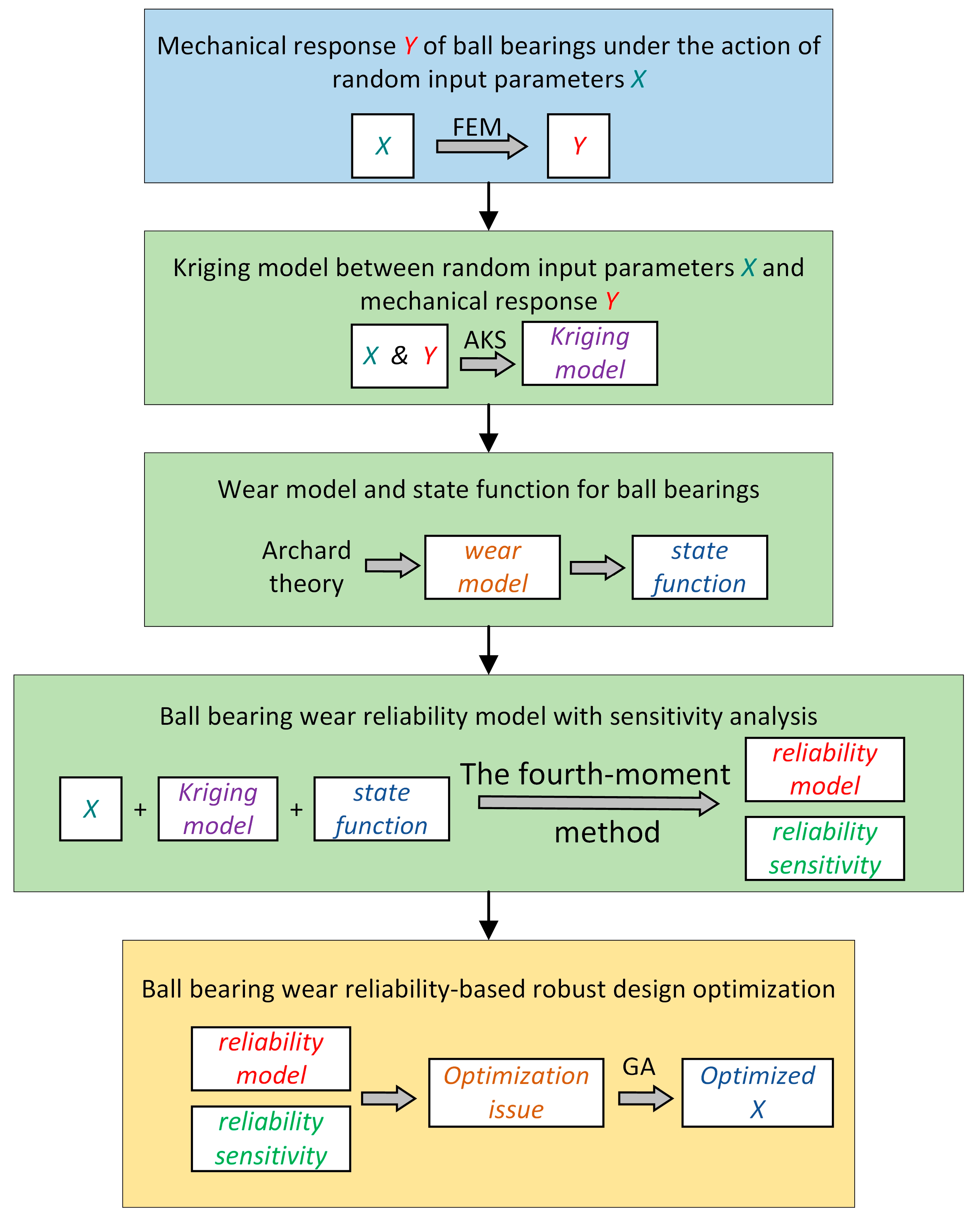
2. Materials and Methods

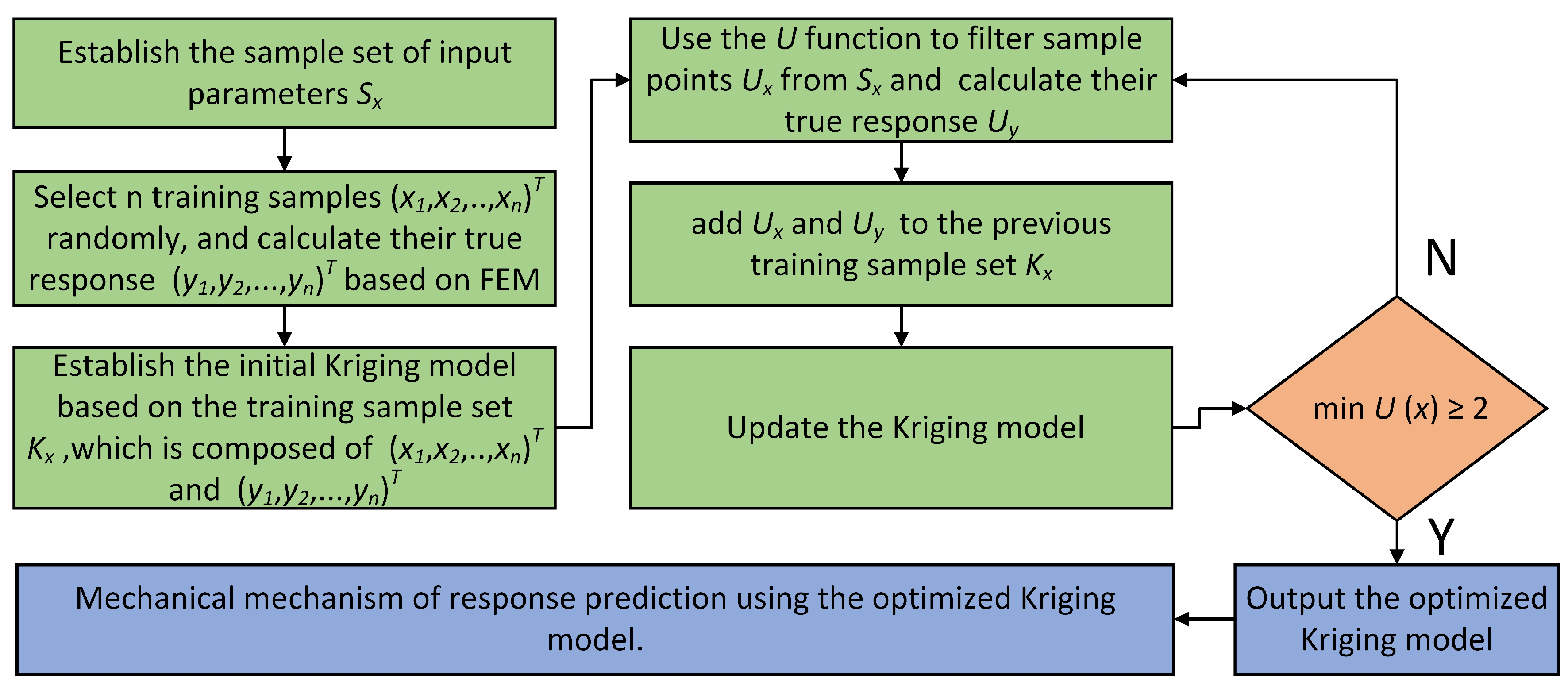
2.1. Kriging Surrogate Model of Mechanical Structural Response Based on FEM

The well-known finite element method (FEM) is commonly used for mechanical analysis of structures due to its high calculation accuracy. It can also be applied to analyze the precise mechanical response of complex mechanical products under dynamic loading. As shown in Figure 2, the ball bearing FEM model is modeled in 3D by CATIA 2020 and imported into Abaqus 2020 to establish the FEM model. Due to the existence of a large number of curved surfaces inside the bearing, a tetrahedral mesh is selected for the ball and cage to ensure the mesh quality required for computational accuracy. However, its application becomes challenging when dealing with a large number of analyses involving stochastic parameters as it requires significant time and computational resources.

A possible approach to address the aforementioned challenges is to combine the FEM with the Kriging method. This method utilizes the training sample set to construct a surrogate model that relates the input design variables to the output mechanical response. Subsequently, it predicts the response value of the estimated point set. Let us consider a sample input variableset for the ball bearing, $x={\left(x_1,x_2,\dots ,x_n\right)}^T$, and the output mechanical response set computed by the FEM is denoted as $y=y\left(x\right)$. The surrogate model between $x$ and $y$ constructed using the Kriging method [37] can be expressed as follows:

$$y\left(x\right)=f^T\left(x\right)\beta +z\left(x\right)$$

(1)

where, $f^T\left(x\right)$ is the polynomial function of $x$, namely the regression model, which serves to establish the global approximate relationship between $x$ and $y$. The regression coefficient corresponding to $x$ is $\beta$; $z\left(x\right)$ refers to a stochastic variable utilized to approximate the deviation in local simulation, with its properties expressed as follows:

$$\left\{\begin{array}{c}E\left[z\left(x\right)\right]=0\\ Var\left[z\left(x\right)\right]={{\sigma }_z}^2\\ Cov\left[z\left(x_i\right),z\left(x_j\right)\right]={{\sigma }_z}^2\left[R_{ij}\left(x_i,x_j\right)\right]\end{array}\right.$$

(2)

In Equation (2), ${{\sigma }_z}^2$ is the variance; $R_{ij}\left(x_i,x_j\right)$ is the correlation function between $x_i$ and $x_j$; and the commonly used correlation function expression is

$$R_{ij}\left(x_i,x_j\right)=\exp \left(-{\displaystyle \sum }_{r=1}^s{\lambda }_r{\left|{x_i}^r-{x_j}^r\right|}^2\right)$$

(3)

where ${\lambda }_r\left(r=1,2,\dots ,s\right)$ represents the correlation coefficient of $x_i$ and $x_j$, and $s$ is the number of variables.

The variance of the $z\left(x\right)$ can be expressed as

$${{\sigma }_z}^2={\displaystyle \frac{1}{N}}{\left(y-J\beta \right)}^T{R}^{-1}\left(y-J\beta \right)$$

(4)

where $N$ refers to the aggregate number of sampling points, $J$ indicates the regression matrix for these sample points, and $R$ denotes the matrix assembled of $R_{ij}\left(x_i,x_j\right)$.

The estimation of the regression coefficient $\beta$ in Equation (1) can be performed using the least squares approach as given by:

$$\widehat{\beta }=\left(J^T{R}^{-1}J\right)J^T{R}^{-1}y$$

(5)

Consequently, the predicted response at the unknown point $x_u$ can be articulated as:

$$g_K\left(x_u\right)=f^T\left(x_u\right)\widehat{\beta }+r^T\left(x_u\right)R^{-1}\left(g-J\widehat{\beta }\right)$$

(6)

In Equation (6), $r$ denotes the vector of correlation functions between the unknown point $x_u$ and the training sample set of parameters

The correlation coefficients, represented as ${\lambda }_r={\left[{\lambda }_1,{\lambda }_2,\dots ,{\lambda }_s\right]}^T$, can be estimated using the maximum-likelihood method, which is expressed by the function:

$$\max F\left(\lambda \right)={\displaystyle \frac{\ln \left({{\sigma }_z}^2\right)+\ln \left|R\right|}{2}}, {\lambda }_r\ge 0\left(r=1,2,\dots ,s\right)$$

(7)

By integrating the obtained ${\lambda }_r$ into Equation (6), a surrogate model can be derived that achieves the highest fitting accuracy based on the current training dataset.

To ensure the Kriging model maintains sufficient accuracy, continual updates to the model are essential. In this paper, in order to establish this adaptive Kriging model, a $U$ learning function [38] is selected and expressed as

$$U\left(x\right)=\left|{\displaystyle \frac{{\mu }_{g_K}\left(x\right)}{{\sigma }_{g_K}\left(x\right)}}\right|$$

(8)

$\min U\left(x\right)\ge 2$ is usually chosen as the convergence judgment basis for the updating process [39]. The specific steps of the adaptive Kriging model using the FEM are shown in Figure 3.

2.2. Wear Reliability Model of Rolling Ball Bearing

The wear failure of ball bearings often occurs under the condition of heavy load and low speed, such as speeds below 1000 rpm, while the load exceeds the dynamic load rating of the bearing. In this case, the wear $H_{ti/to}$ between the balls and the inner/outer ring of the bearing in time $t$ can be calculated by the Archard wear theory [40] as follows:

$$H_{ti/to}=\Delta h_{i/o}\times J_{i/o}\times t$$

(9)

where $J_{i/o}$ is the number of contact cycles per unit time. $\Delta h$ is the wear depth at the distance from the semi-axis x of the contact ellipse and can be obtained as follows:

$$\Delta h=G_0{\left({\displaystyle \frac{\sigma }{HB}}\right)}^m{L}_x$$

(10)

In Equation (10), $HB$ is the hardness of the material. $\sigma$ is the contact stress obtained through the adaptive Kriging model. $L_x$ is the slip distance of each contact between the ball and the inner/outer ring. $G_0$ is called the wear constant, which can be calculated as follows:

$$G_0=k{\left({\displaystyle \frac{\xi \left(f\right)}{{\epsilon }_0}}\right)}^m{\left({\displaystyle \frac{R_{max}}{r_{\rho }{\psi }^{1/\vartheta }}}\right)}^c$$

(11)

where ${\epsilon }_0$ represents the elongation at break in the material. $r_{\rho }$ denotes the radius of curvature, and $R_{max}$ refers to the highest point of the micro-convex body on the contact surface. The curvature coefficients of the support surface are represented by $\psi$ and $\vartheta$. $k$, $m$, and $c$ are empirical constants. $\xi \left(f\right)$ is the influence factor of lubricant on the contact area, which needs to be selected according to the specific contact zone lubrication [5].

The slip distance $L_x$ in Equation (10) can be approximated according to the elliptic contact and velocity distribution law as follows:

$$L_x\approx b_x\left[{\left({\displaystyle \frac{0.348a}{R_b}}\right)}^2-{\left({\displaystyle \frac{x}{R_b}}\right)}^2\right]$$

(12)

where $b_x$ is the half-length perpendicular to the x direction at the point ($x$, $y$). $R_b$ is the radius of the ball. $a$ is the long half axis of the ellipse.

The number of contact cycles $J_{i/o}$ in Equation (9) can be calculated as

$$J_{i/o}={\displaystyle \frac{Z}{2}}\left(n_o-n_i\right)\left(1\pm {\displaystyle \frac{D_b}{D_m}}\right)$$

(13)

where, $n_i$ and $n_o$ are the rotation speeds of the inner and outer ring, respectively. $D_b$ and $D_m$ are the diameter of ball and pitch circle, respectively.

In the case of ball bearings, the wear between the ball and the inner/outer ring causes the bearing clearance to gradually increase. This increase in clearance further exacerbates the vibration and noise. Hence, the bearing clearance can serve as an indicator to assess the extent of bearing wear. Consequently, the wear reliability of the ball bearing can be expressed as:

$$g\left(\mathit{X}\right)=\overline{H}-\left[H_i\left(\mathit{X},t\right)+H_o\left(\mathit{X},t\right)\right]-C_0$$

(14)

In Equation (14), $\mathit{X}={\left(X_1,X_2,···,X_n\right)}^T$ represents the vector composed of input design parameters. $H_i\left(\mathit{X},t\right)$ and $H_o\left(\mathit{X},t\right)$ are, respectively, the total amount of wear between the ball and the inner and outer ring after time $t$. $C_0$ is the initial radial clearance, which can be determined according to the specific accuracy level of the bearing, and its measurement method refers to Standard GB/T 25769-2010 [41]. $\overline{H}$ is the wear threshold and can be determined with reference to the radial permissible clearance of rolling bearings, as shown in

Table 1. Maximum allowable wear clearance of rolling bearings.

Inner Diameter $\mathit{D}$ (mm)	Radial Clearance ${\overline{\mathit{H}}}_{\mathit{r}}$ (mm)	Axial Clearance ${\overline{\mathit{H}}}_{\mathit{a}}$ (mm)
<30	4D/1000	0.2
35~70	3.5D/1000	0.3
75~100	3D/1000	0.3
>100	<0.3	0.3

[42].

Since the fourth-moment method has been proved to be more accurate than the FOSM [25], the wear reliability model of ball bearings based on the fourth-moment method is constructed in this paper.

Applying the stochastic perturbation theory to the ball bearing wear state function, the mean ${\mu }_g$, variance ${{\sigma }_g}^2$, third moment ${\xi }_g$ and fourth moment ${\eta }_g$ of the corresponding state function can be expressed as follows:

$${\mu }_g=\mathrm{E}\left(g\left(\mathit{X}\right)\right)=g\left({\mu }_{\mathit{X}}\right)$$

(15)

$${{\sigma }_g}^2=\mathrm{E}\left[{\left(g\left(\mathit{X}\right)-{\mu }_g\right)}^2\right]={\displaystyle \frac{\partial g\left({\mu }_{\mathit{X}}\right)}{\partial {\mathit{X}}^T}}{C}_2\left(\mathit{X}\right){\displaystyle \frac{\partial g\left({\mu }_{\mathit{X}}\right)}{\partial \mathit{X}}}$$

(16)

$${\xi }_g=\mathrm{E}\left[{\left(g\left(\mathit{X}\right)-{\mu }_g\right)}^3\right]={\displaystyle \frac{\partial g\left({\mu }_{\mathit{X}}\right)}{\partial {\mathit{X}}^T}}{C}_3\left(\mathit{X}\right){\displaystyle \frac{\partial g\left({\mu }_{\mathit{X}}\right)}{\partial \mathit{X}}}\otimes {\displaystyle \frac{\partial g\left({\mu }_{\mathit{X}}\right)}{\partial \mathit{X}}}$$

(17)

$${\eta }_g=\mathrm{E}\left[{\left(g\left(\mathit{X}\right)-{\mu }_g\right)}^4\right]={\displaystyle \frac{\partial g\left({\mu }_{\mathit{X}}\right)}{\partial {\mathit{X}}^T}}\otimes {\displaystyle \frac{\partial g\left({\mu }_{\mathit{X}}\right)}{\partial {\mathit{X}}^T}}{C}_4\left(\mathit{X}\right){\displaystyle \frac{\partial g\left({\mu }_{\mathit{X}}\right)}{\partial \mathit{X}}}\otimes {\displaystyle \frac{\partial g\left({\mu }_{\mathit{X}}\right)}{\partial \mathit{X}}}$$

(18)

where ${\mathit{\mu }}_X$, $C_2\left(\mathit{X}\right)$, $C_3\left(\mathit{X}\right),$ and $C_4\left(\mathit{X}\right)$ denote the mean vector, second moment matrix, third moment matrix, and fourth moment matrix of input parameter vector $\mathit{X}$, respectively. $\mathit{A}\otimes \mathit{B}$ denote the Kronecker product of $\mathit{A}$ and $\mathit{B}$.

When the first four moments of the input parameter vector $\mathit{X}$ are known, the first four moments of the ball bearing wear state function can be obtained according to Equations (15)–(18), and then the corresponding reliability index ${\beta }_{FMt}$ can be obtained according to the fourth-moment method [25] as follows:

$${\beta }_{FMt}={\displaystyle \frac{3\left(3{\eta }_g+{{\sigma }_g}^4\right){\mu }_g+5{\xi }_g\left({{\mu }_g}^2-{{\sigma }_g}^2\right)}{\sqrt{9{\left(3{\eta }_g+{{\sigma }_g}^4\right)}^2{{\sigma }_g}^2-5{{\xi }_g}^2\left(13{\eta }_g+11{{\sigma }_g}^4\right)}}}$$

(19)

Further, the wear reliability of ball bearings at time t, $R_{FMt}$, can be approximated as follows:

$$R_{FMt}=\mathsf{\Phi }\left({\beta }_{FMt}\right)$$

(20)

where $\mathsf{\Phi }\left(·\right)$ denotes the standard normal distribution function.

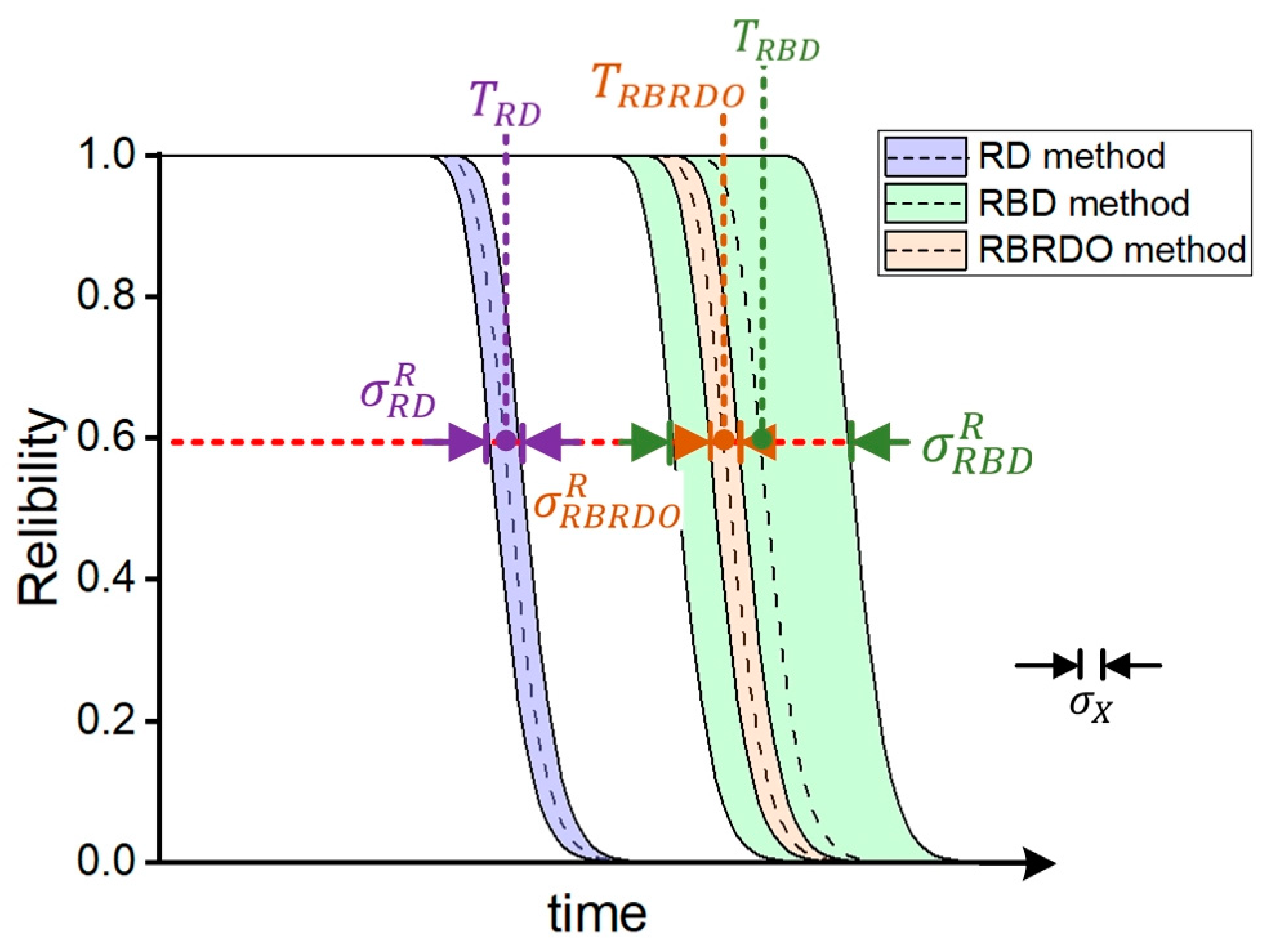
2.3. Sensitivity Analysis and Reliability-Based Robust Design

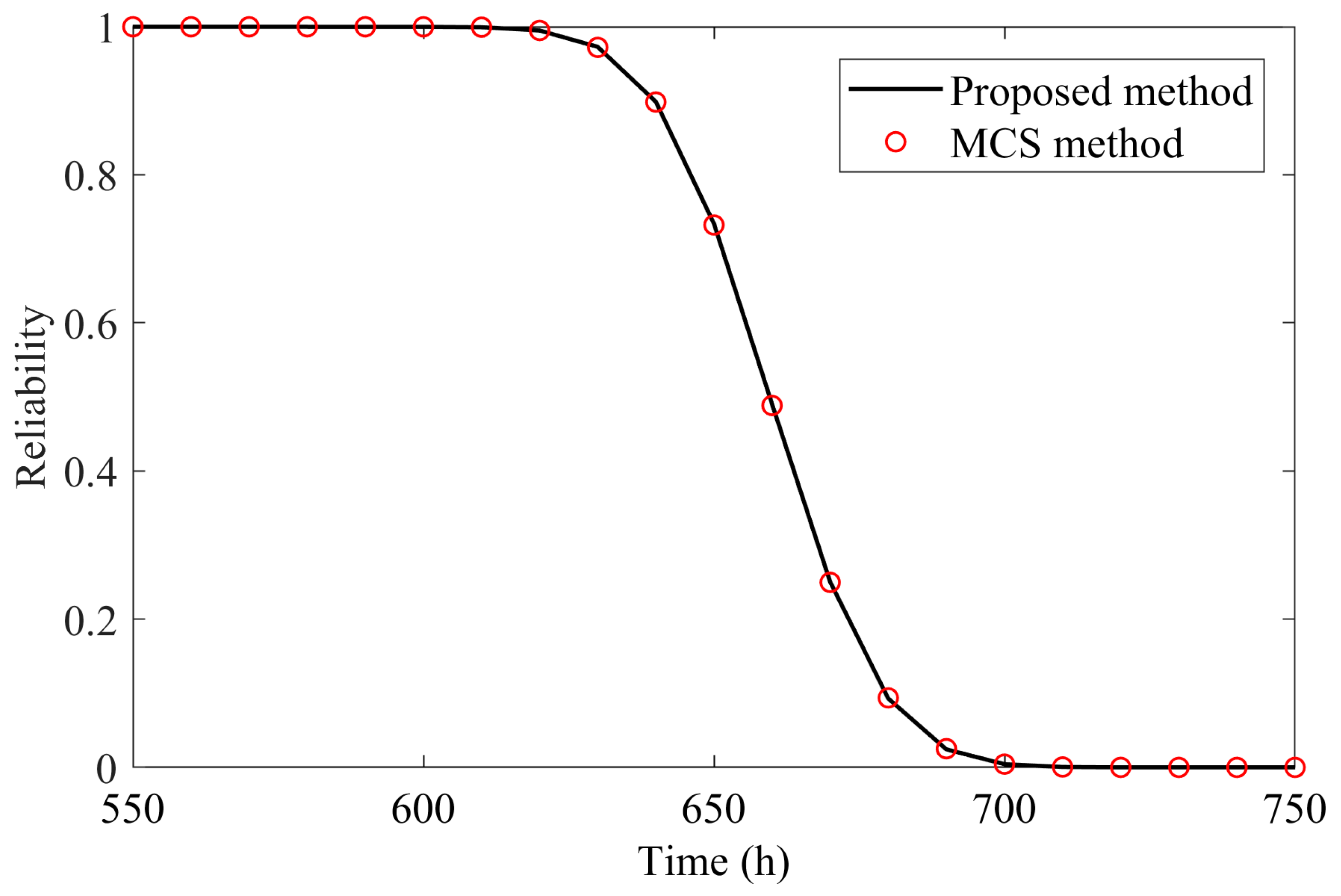
Reliability sensitivity analysis is a quantitative method used to assess the impact of random changes in input variables on reliability [43]. In practical engineering design, if a certain input parameter of the ball bearing exhibits a significant influence on wear reliability due to random variations, it should be controlled during the production process in accordance with economic and design requirements. Conversely, if the random variation of the parameter has a lesser impact on wear reliability, it can be considered a deterministic variable, allowing for a reduction in design parameters. Therefore, conducting sensitivity analysis on the wear reliability of ball bearings holds engineering significance.

Usually, in order to guide the design and processing of mechanical products, only the sensitivity of reliability to the mean and variance of random input parameters is analyzed [44]. According to the fourth-moment method [45], the sensitivity of ball bearing wear reliability to the mean ${{\mu }_{\mathit{X}}}^T$ and variance ${{\sigma }_{\mathit{X}}^2}^T$ of the input parameter vector $\mathit{X}$ can be derived as follows:

$${\displaystyle \frac{\partial R_{FMt}}{\partial {{\mu }_{\mathit{X}}}^T}}={\displaystyle \frac{\partial R_{FMt}}{\partial {\beta }_{FMt}}}\left[{\displaystyle \frac{\partial {\beta }_{FMt}}{\partial {\mu }_g}}{\displaystyle \frac{\partial {\mu }_g}{\partial {{\mu }_{\mathit{X}}}^T}}+{\displaystyle \frac{\partial {\beta }_{FMt}}{\partial {\sigma }_g^2}}{\displaystyle \frac{\partial {\sigma }_g^2}{\partial {{\mu }_{\mathit{X}}}^T}}+{\displaystyle \frac{\partial {\beta }_{FMt}}{\partial {\xi }_g}}{\displaystyle \frac{\partial {\xi }_g}{\partial {{\mu }_{\mathit{X}}}^T}}+{\displaystyle \frac{\partial {\beta }_{FMt}}{\partial {\eta }_g}}{\displaystyle \frac{\partial {\eta }_g}{\partial {{\mu }_{\mathit{X}}}^T}}\right]$$

(21)

$${\displaystyle \frac{\partial R_{FMt}}{\partial {{\sigma }_{\mathit{X}}^2}^T}}={\displaystyle \frac{\partial R_{FMt}}{\partial {\beta }_{FMt}}}\left[{\displaystyle \frac{\partial {\beta }_{FMt}}{\partial {\mu }_g}}{\displaystyle \frac{\partial {\mu }_g}{\partial {{\sigma }_{\mathit{X}}^2}^T}}+{\displaystyle \frac{\partial {\beta }_{FMt}}{\partial {\sigma }_g^2}}{\displaystyle \frac{\partial {\sigma }_g^2}{\partial {{\sigma }_{\mathit{X}}^2}^T}}+{\displaystyle \frac{\partial {\beta }_{FMt}}{\partial {\xi }_g}}{\displaystyle \frac{\partial {\xi }_g}{\partial {{\sigma }_{\mathit{X}}^2}^T}}+{\displaystyle \frac{\partial {\beta }_{FMt}}{\partial {\eta }_g}}{\displaystyle \frac{\partial {\eta }_g}{\partial {{\sigma }_{\mathit{X}}^2}^T}}\right]$$

(22)

The derivative ${\displaystyle \frac{\partial R_{FMt}}{\partial {\beta }_{FMt}}}$ can be calculated as follows:

$${\displaystyle \frac{\partial R_{FMt}}{\partial {\beta }_{FMt}}}=\varphi \left({\beta }_{FMt}\right)$$

(23)

where $\varphi \left(·\right)$ is the probability density function of the standard normal distribution. The equations for calculating the unknown differential in Equations (21) and (22) are shown in Appendix A. Generally, a reliability sensitivity gradient is used to comprehensively consider the sensitivity of reliability to the mean and variance of input parameters.

$$\mathrm{grad}\left(R_{FMt}\right)=\sqrt{{\left({\displaystyle \frac{\partial R_{FMt}}{\partial {{\mu }_{\mathit{X}}}^T}}\right)}^2+{\left({\displaystyle \frac{\partial R_{FMt}}{\partial {{\sigma }_{\mathit{X}}^2}^T}}\right)}^2}$$

(24)

The main idea of traditional RBRDO is to take the reliability and reliability variance as optimization function, but for ball bearing products, it is often required that the reliability reaches a certain index within a certain working time. Therefore, the objective of ball bearings wear RBRDO is to minimize the reliability sensitivity gradient when the reliability target is met within the required life time. The reliability and reliability sensitivity gradients are brought into the RBRDO model for calculation, and the proposed RBRDO model can be expressed as follows:

$$\left\{\begin{array}{c}\begin{array}{c}min f\left(\mathit{X}\right)=\mathrm{grad}\left(R_{FMt}\right)\\ s.t.R_{FMt}-R_0\ge 0\end{array}\\ \begin{array}{c}{p}_i\left({\mu }_{\mathit{X}}\right)\ge 0,i=1,\dots ,p\\ q_i\left({\mu }_{\mathit{X}}\right)=0,j=1,\dots ,q\end{array}\end{array}\right.$$

(25)

where $R_0$ denotes the specified reliability requirement; $p_i\left({\mu }_{\mathit{X}}\right)$ and $q_i\left({\mu }_{\mathit{X}}\right)$ indicate the inequality and equality constraints, respectively. The optimization problems described can be addressed through different optimization techniques or mathematical software such as the genetic algorithm or the MATLAB 2018 optimization toolbox.

3. Results

To realize the wear reliability RBRDO of ball bearings, a series of five consecutive steps (illustrated in Figure 4) must be executed. Initially, the mechanical response $\mathit{Y}$ of the rolling ball bearing is derived using the finite element method based on the input parameters $\mathit{X}$. Next, a surrogate model that relates $\mathit{X}$ to $\mathit{Y}$ is developed employing the adaptive Kriging approach. Subsequently, the wear model for the rolling ball bearing is formulated according to Archard’s theory, and a wear state equation is introduced. Finally, the wear reliability model for the rolling ball bearing is solved utilizing the fourth-moment method, followed by a sensitivity analysis. Finally, RBRDO is performed for ball bearing wear reliability and design result parameters are output.

Deep groove ball bearing 6016 was selected as the optimization object with the following conditions: outer diameter $D=125 \mathrm{mm}$, inner diameter $d=80 \mathrm{mm}$, the number of balls $\mathrm{Z}=20$, rotating speed $\mathrm{n}=1000 \mathrm{r}/\min$, radial force $F_r=500 \mathrm{N}$, axial preload $10 \mathrm{N}$, material GCr15.

Design variables associated with the wear calculation were selected to construct the vector $\mathit{X}={\left[D_m, D_w, R_i, R_o, E, v, HB, G_0\right]}^T$. Ten 6016 bearings of the same manufacturer with the same accuracy were measured with a CMM to obtain the parameter data, and the first fourth-order moments of the parameter in $\mathit{X}$ were obtained based on the calculation of these 10 sets of data, and the rest of the parameters were obtained according to the method described in the reference [10], as shown in

Table 2. 6016 Bearing input parameters with first fourth-order moments.

Bearing Parameters	Mean	Variance	Skewness	Kurtosis
Center circle diameter $D_m$ (mm)	102.4874	2.5 × 10−5	9.96 × 10−2	2.87
Ball diameter$D_w$ (mm)	13.4940	4.0 × 10−6	4.09 × 10−2	2.96
Inner ring groove radius $R_i \left(\mathrm{mm}\right)$	7.1010	1.0 × 10−6	−7.37 × 10−2	3.03
Outer ring groove radius $R_o$ (mm)	6.9960	1.0 × 10−6	1.29 × 10−1	2.69
Elastic modulus $E$ (GPa)	208	1.0 × 10−4	−1.88 × 10−4	3.47
Poisson’s ratio $v$	0.3	1.0 × 10−8	−1.53 × 10−1	2.85
Hardness $HB$	200	1.0 × 10−4	8.35 × 10−2	2.88
Initial radial clearance $G_0$	0.0240	2.5 × 10−5	6.46 × 10−2	2.92

.

As shown in Figure 5, random input parameters of bearing 6016 are generated based on Table 2, and the corresponding mechanical response is calculated by ABAQUS/CAE 2020. Multiple sets of input parameters and corresponding mechanical responses are composed of a training dataset, through which adaptive Kriging updating is performed to obtain the optimal Kriging model. Subsequently, with the assumption that the first four moments of the input parameters are established, the Kriging model is integrated with the wear state function of the ball bearing, and the first four moments of the wear state function can be derived.

Ultimately, these moments were substituted into Equations (19) and (20) at various time intervals to generate the reliability curve for ball bearing wear, illustrated in Figure 6.

The moment $t_d=635 \mathrm{h}$, near 95% reliability in the reliability reduction process, is selected, and the reliability calculation results under this moment are shown in

Table 3. Reliability calculations for the proposed method and MCS at time $t_d$.

Methods	${\mathit{t}}_{\mathit{d}}$	${\mathit{\beta }}_{{\mathit{t}}_{\mathit{d}}}$	${\mathit{R}}_{{\mathit{t}}_{\mathit{d}}}$	Relative Error
FOSM method	635 h	−1.6567	95.12%	0.7521%
The proposed method	635 h	−1.5985	94.50%	0.0953%
MCS method	635 h	\	94.41%	\

.

Assuming that the dimensional parameters follow a normal distribution, based on the mean and variance data in Table 2, we can perform the Monte Carlo simulation (MCS) reliability calculation, and the reliability curve obtained was compared with the proposed method in the time period of 550–750 h, as shown in Figure 7. It can be seen that the reliability results of the proposed method are highly consistent with those of the MCS method. According to Table 3, the relative error between the reliability result of the proposed method and that of the MCS method at $t_d$ is 0.0953%, which is much smaller than the relative error between the reliability results of the conventional FOSM method and those of the MCS method. The sample size of the MCS method used is ${10}^5$, which can be regarded as an exact solution. Therefore, the accuracy of the proposed method is proved. In addition, the proposed method has obvious efficiency advantages compared with the MCS method, which needs to calculate the state function ${10}^5$ times.

Based on Equations (21) and (22), the sensitivity of ball bearing wear reliability to the mean value and variance of input parameters can be obtained, as shown in

Table 4. Sensitivity of rolling bearing wear reliability to input parameters.

Input Parameters	Reliability Sensitivity		Sensitivity Gradient
	$\frac{\partial {\mathit{R}}_{\mathit{F}\mathit{M}\mathit{t}}}{\partial {\mathit{\mu }}_{\mathit{X}\mathit{i}}}$	$\frac{\partial {\mathit{R}}_{\mathit{F}\mathit{M}\mathit{t}}}{\partial {\mathit{\sigma }}_{\mathit{X}\mathit{i}}^2}$	$\mathbf{grad} \left({\mathit{R}}_{\mathit{F}\mathit{M}\mathit{t}}\right)$
Center circle diameter $D_m$	0.0037	−1.06 × 10−6	40.4176
Ball diameter $D_w$	2.2782	−0.1616
Inner ring groove radius $R_i$	−1.1763	−0.0215
Outer ring groove radius $R_o$	−4.4164	−0.3036
Elastic modulus $E$	−0.0028	−1.21 × 10−6
Poisson’s ratio $v$	−0.3828	−2.28 × 10−4
Hardness $HB$	−0.0283	−1.25 × 10−4
Initial radial clearance $G_0$	20.9554	−34.1776

, and the sensitivity gradient is calculated by Equation (24).

Table 4 shows the sensitivity of reliability relative to the mean values of $D_m$, $D_w,$ and $G_0$ is positive, while it exhibits a negative sensitivity regarding the mean values of $R_i$, $R_o$, $E$, $v,$ and $HB$. This means that the reliability increases when the mean values of $D_m$, $D_w$, and $G_0$ increase within the permitted initial value interval and decreases as the mean values of $R_i$, $R_o$, $E$, $v,$ and $HB$ increase. In addition, the sensitivity of reliability to the variance of all parameters is also negative. This implies that as the variance of any given input parameter rises, there is a corresponding decrease in reliability.

In order to facilitate comparison of the reliability sensitivity of different parameters, the sensitivity $\lg {\displaystyle \frac{\partial R_{FMt}}{\partial {\mu }_{\mathit{X}\mathit{i}}}}$ of reliability to the mean and the sensitivity $\lg {\displaystyle \frac{\partial R_{FMt}}{\partial {\sigma }_{\mathit{X}\mathit{i}}^2}}$ of reliability to variance were obtained by taking the absolute values and calculating their logarithms, respectively, as shown in Figure 8, where $\lg \left(·\right)$ denotes logarithmic base 10. It can be seen from Figure 8 that on the one hand, the sensitivity of reliability to the mean and variance of $G_0$ is the largest of all parameters, followed by $R_o$, $R_i$ and $D_w$. Therefore, the mean and variance of these parameters need to be regulated according to economic and design requirements. On the other hand, reliability is less sensitive to the mean and variance of $v$, $E$, $HB,$ and $D_m$, so it can be appropriately treated as a constant value to reduce the number of design parameters.

Based on the reliability and sensitivity at the $t_d$, it is possible to perform RBRDO for ball bearing wear, starting with the determination of constraints for ball bearings as follows:

• The wear reliability target for ball bearings is set to $R_0=0.999$, which means that the optimized reliability result $R_{t_d}^{\prime }$ obtained at the moment $t_d$ should be no less than $R_0$. Therefore, the reliability constraint is expressed as follows:

  $$R_0-R_{t_d}^{\prime }\le 0$$

  (26)
• In order to ensure the point contact between the inner/outer raceway and the balls, the inner/outer raceway radius $R_i/R_o$ should be larger than the ball radius $D_w$, and the inner raceway radius $R_i$ is usually larger than the outer raceway radius $R_o$. According to the above principles to establish constraints as follows:

  $$0.5D_w<R_o<R_i$$

  (27)
• Based on the structural design requirements of ball bearings and with reference to the various dimensional standards for ball bearings [46], the initial value constraints are established for the input parameters $\mathit{X}$ as follows:

  $$\begin{array}{c}\begin{array}{c}\begin{array}{c}102.30<D_m<102.70\\ 13.40<D_w<13.60\end{array}\\ \begin{array}{c}7.00<R_i<7.20\\ 6.90<R_o<7.10\end{array}\end{array}\\ \begin{array}{c}\begin{array}{c}207.00<E<209.00\\ 0.25<v<0.35\end{array}\\ \begin{array}{c}198.00<HB<200.00\\ 0.0235<G_0<0.0245\end{array}\end{array}\end{array}$$

  (28)

After establishing the above constraints, the optimization model can be solved by genetic algorithm or other optimization algorithms, and the optimization parameters obtained from the solution are shown in

Table 5. The optimized design parameters of bearing 6016.

Input Parameters	Before Optimization	After Optimization
Center circle diameter $D_m$ (mm)	102.4874	102.4306
Ball diameter $D_w$ (mm)	13.4940	13.4501
Inner ring groove radius $R_i \left(\mathrm{mm}\right)$	7.1010	7.1499
Outer ring groove radius $R_o$ (mm)	6.9960	7.05
Elastic modulus $E$ (GPa)	208	208.0212
Poisson’s ratio $v$	0.3	0.3497
Hardness $HB$	200	201.9952
Initial radial clearance $G_0$	0.0240	0.0235

.

Based on the results of the optimized parameters in Table 5, the optimized wear reliability curves are calculated and compared with the pre-optimized ones, as shown in Figure 9. In addition, the wear reliability sensitivity gradient for the optimized 6016 bearing is calculated, as shown in

Table 6. Reliability and sensitivity gradient comparison before and after optimization.

Input Parameters	${\mathit{t}}_{\mathit{d}}$	${\mathit{\beta }}_{{\mathit{t}}_{\mathit{d}}}$	${\mathit{R}}_{{\mathit{t}}_{\mathit{d}}}$	$\mathbf{g}\mathbf{r}\mathbf{a}\mathbf{d} \left({\mathit{R}}_{\mathit{F}\mathit{M}\mathit{t}}\right)$
Before optimization	635 h	−1.5985	94.50%	40.4176
After optimization	635 h	−5.5483	99.99%	8.4755 × 10−5

.

According to Figure 9, the reliability results of the optimized 6016 bearing wear are considerably improved compared to the pre-optimization results, indicating a more reasonable structural design of the ball bearing. This is further supported by the achievement of the constraint target $R_0$ at moment $t_d$, as shown in Table 6. The optimized reliability sensitivity gradient in Table 6 shows a significant reduction, suggesting the attainment of more robust results and validating the effectiveness of the proposed method.

In order to facilitate the observation of the changes in reliability sensitivity of different parameters before and after the optimization, the reliability sensitivities were taken as absolute values and their logarithms were calculated, and the sensitivity $\lg {{\displaystyle \frac{\partial R_{FMt}}{\partial {\mu }_{Xi}}}}^{op}$ of reliability to the mean and the sensitivity $\lg {{\displaystyle \frac{\partial R_{FMt}}{\partial {\sigma }_{Xi}^2}}}^{op}$ of reliability to variance under the optimized parameters were obtained as shown in Figure 10. It can be seen that the sensitivities of the same parameters are significantly reduced after optimization, while the relationship between the magnitude of the sensitivities of different parameters is basically the same as before optimization. This indicates that the reliability of the optimized 6016 bearing is less sensitive to changes in the design variables, which shows that the 6016 bearing has better robustness after optimization with the method proposed in this paper.

The results obtained from the analysis of the 6016 bearing demonstrate that the proposed method significantly reduces the sensitivity of reliability while meeting the specified reliability index for wear of the rolling bearing over the designated operating period. This indicates that the reliability requirements are satisfied and the robustness is effectively maximized. The accuracy of the proposed method is validated through comparison with the MCS method. Furthermore, the validity of the proposed method is confirmed by evaluating the reliability and robustness before and after optimizing the design parameters. Although the numerical examples provided in this study focus on reliability analysis under constant working conditions, the proposed method is also applicable for reliability analysis and design under variable load conditions.

4. Conclusions

In this paper, we apply the reliability-based robust design optimization method with the fourth-moment method to analyze ball bearing wear. We propose a new wear design method for ball bearings that overcomes the limitations of existing methods. The existing RBRDO based on the fourth-moment method faces difficulties in obtaining the explicit wear state function of ball bearings. By combining the finite element method with the Kriging method, we are able to obtain the explicit wear state equation of ball bearings. Our method also enables wear reliability sensitivity analysis and reliability-based robust optimization of ball bearings. We demonstrate the effectiveness of our proposed method through an example of a 6016 bearing. The reliability results obtained using our method at selected time points have minimal error compared to the MCS method. Furthermore, the optimization significantly reduces the reliability sensitivity gradient, further validating the accuracy and effectiveness of our proposed method.

The contribution of our method lies in the implementation of wear reliability sensitivity analysis and robust reliability-based optimization for ball bearings, which overcomes the limitation of the existing fourth-order moment reliability methods that make it difficult to obtain the explicit wear state function of ball bearings. In addition, the method can take into account economic factors by weighting the reliability sensitivity according to the processing cost of different sizing parameters.

However, it is important to note that the accuracy of the FEM model plays a crucial role in obtaining reliable results. Therefore, a thorough understanding of the designed structure and its corresponding failure mechanism is essential in the design process.

The method proposed in this paper can be improved in the future from the following two specific aspects. (1) Constructing a realistic correlation between bearing wear and the Archard wear model by conducting specific wear tests on relevant bearing products, so as to improve the accuracy of the method. (2) Processing and manufacturing bearing test samples according to the design results and carrying out several sets of comparison tests with the bearing products before optimization so as to further clarify the design optimization effect.

References

1. Weibull, W. Efficient Methods for Estimating Fatigue Life Distribution of Rolling Bearings; Elsevier: New York, NY, USA, 1962; pp. 252–265. [Google Scholar]
2. Lundberg, G.; Palmgren, A. Dynamic capacity of rolling bearings. J. Appl. Mech. 1949, 16, 165–172. [Google Scholar] [CrossRef]
3. Organización Internacional de Normalización. Rolling Bearings: Dynamic Load Ratings and Rating Life; ISO: Geneva, Switzerland, 2007. [Google Scholar]
4. Ding, N.; Yan, S.; Ma, G.; Li, H.; Jiang, D. Mixed thermo-elasto-hydrodynamic lubrication and wear coupling simulation analysis for dynamical load journal bearings. Proc. Inst. Mech. Eng. Part C J. Mech. Eng. Sci. 2023, 237, 6020–6041. [Google Scholar] [CrossRef]
5. Wang, X.; Wang, B.; Chang, M.; Li, L. Reliability and sensitivity analysis for bearings considering the correlation of multiple failure modes by mixed Copula function. Proc. Inst. Mech. Eng. Part O J. Risk Reliab. 2019, 234, 15–26. [Google Scholar] [CrossRef]
6. Li, X.; Yan, K.; Lv, Y.; Yan, B.; Dong, L.; Hong, J. Study on the influence of machine tool spindle radial error motion resulted from bearing outer ring tilting assembly. Proc. Inst. Mech. Eng. Part C J. Mech. Eng. Sci. 2019, 233, 3246–3258. [Google Scholar] [CrossRef]
7. Zhang, T.; He, D. An improved high-order statistical moment method for structural reliability analysis with insufficient data. Proc. Inst. Mech. Eng. Part C J. Mech. Eng. Sci. 2017, 232, 1050–1056. [Google Scholar] [CrossRef]
8. Li, Z.; Tian, G.; Cheng, G.; Liu, H.; Cheng, Z. An integrated cultural particle swarm algorithm for multi-objective reliability-based design optimization. Proc. Inst. Mech. Eng. Part C J. Mech. Eng. Sci. 2013, 228, 1185–1196. [Google Scholar] [CrossRef]
9. Gao, Y.; Zhang, F.; Li, Y. Reliability optimization design of a planar multi-body system with two clearance joints based on reliability sensitivity analysis. Proc. Inst. Mech. Eng. Part C J. Mech. Eng. Sci. 2018, 233, 1369–1382. [Google Scholar] [CrossRef]
10. E, S.; Wang, Y.; Xie, B.; Lu, F. A Reliability-Based Robust Design Optimization Method for Rolling Bearing Fatigue under Cyclic Load Spectrum. Mathematics 2023, 11, 2843. [Google Scholar] [CrossRef]
11. Winkler, A.; Marian, M.; Tremmel, S.; Wartzack, S. Numerical modeling of wear in a thrust roller bearing under mixed elastohydrodynamic lubrication. Lubricants 2020, 8, 58. [Google Scholar] [CrossRef]
12. Pozzebon, M.L.; Lin, C.; Meehan, P.A. On the modeling of wear in grease-lubricated spherical roller bearings. Tribol. Trans. 2020, 63, 806–819. [Google Scholar] [CrossRef]
13. Zhao, Y.; Lu, Z.; Ono, T. A simple third-moment method for structural reliability. J. Asian Archit. Build. Eng. 2006, 5, 129–136. [Google Scholar] [CrossRef]
14. Zhao, Y.; Ono, T. Moment methods for structural reliability. Struct. Saf. 2001, 23, 47–75. [Google Scholar] [CrossRef]
15. Clark, D.L., Jr.; Bae, H.; Forster, E.E. Gaussian Surrogate Dimension Reduction for Efficient Reliability-Based Design Optimization. AIAA J. 2020, 58, 4736–4750. [Google Scholar] [CrossRef]
16. Lee, I.; Choi, K.K.; Du, L.; Gorsich, D. Dimension reduction method for reliability-based robust design optimization. Comput. Struct. 2008, 86, 1550–1562. [Google Scholar] [CrossRef]
17. Dauparas, J.; Anishchenko, I.; Bennett, N.; Bai, H.; Ragotte, R.J.; Milles, L.F.; Wicky, B.I.; Courbet, A.; de Haas, R.J.; Bethel, N.; et al. Robust deep learning--based protein sequence design using ProteinMPNN. Science 2022, 378, 49–56. [Google Scholar] [CrossRef] [PubMed]
18. Park, G.; Lee, T.; Lee, K.H.; Hwang, K. Robust design: An overview. AIAA J. 2006, 44, 181–191. [Google Scholar] [CrossRef]
19. Lee, D.; Jahanbin, R.; Rahman, S. Robust design optimization by spline dimensional decomposition. Probabilistic Eng. Mech. 2022, 68, 103218. [Google Scholar] [CrossRef]
20. Park, J.; Yoo, D.; Moon, J.; Yoon, J.; Park, J.; Lee, S.; Lee, D.; Kim, C. Reliability-Based Robust Design Optimization of Lithium-Ion Battery Cells for Maximizing the Energy Density by Increasing Reliability and Robustness. Energies 2021, 14, 6236. [Google Scholar] [CrossRef]
21. Yu, S.; Wang, Z.; Wang, Z. Time-dependent reliability-based robust design optimization using evolutionary algorithm. ASCE-ASME J. Risk Uncertain. Eng. Syst. Part B Mech. Eng. 2019, 5, 20911. [Google Scholar] [CrossRef]
22. Gong, C.; Frangopol, D.M. An efficient time-dependent reliability method. Struct. Saf. 2019, 81, 101864. [Google Scholar] [CrossRef]
23. Yang, W.; Zhang, B.; Wang, W.; Li, C. Time-dependent structural reliability under nonstationary and non-Gaussian processes. Struct. Saf. 2023, 100, 102286. [Google Scholar] [CrossRef]
24. Doltsinis, I.; Kang, Z. Robust design of structures using optimization methods. Comput. Meth. Appl. Mech. Eng. 2004, 193, 2221–2237. [Google Scholar] [CrossRef]
25. Zhang, T. An improved high-moment method for reliability analysis. Struct. Multidiscip. Optim. 2017, 56, 1225–1232. [Google Scholar] [CrossRef]
26. Zhang, T. Robust reliability-based optimization with a moment method for hydraulic pump sealing design. Struct. Multidiscip. Optim. 2018, 58, 1737–1750. [Google Scholar] [CrossRef]
27. Zhang, T.; He, D. A Reliability-Based Robust Design Method for the Sealing of Slipper-Swash Plate Friction Pair in Hydraulic Piston Pump. IEEE Trans. Reliab. 2018, 67, 459–469. [Google Scholar] [CrossRef]
28. Ant O Nio, C.C.C.C.; Hoffbauer, L.I.S.N. An approach for reliability-based robust design optimisation of angle-ply composites. Compos. Struct. 2009, 90, 53–59. [Google Scholar] [CrossRef]
29. Dammak, K.; El Hami, A. Thermal reliability-based design optimization using Kriging model of PCM based pin fin heat sink. Int. J. Heat Mass Transf. 2021, 166, 120745. [Google Scholar] [CrossRef]
30. Tripathy, R.K.; Bilionis, I. Deep UQ: Learning deep neural network surrogate models for high dimensional uncertainty quantification. J. Comput. Phys. 2018, 375, 565–588. [Google Scholar] [CrossRef]
31. White, D.A.; Arrighi, W.J.; Kudo, J.; Watts, S.E. Multiscale topology optimization using neural network surrogate models. Comput. Meth. Appl. Mech. Eng. 2019, 346, 1118–1135. [Google Scholar] [CrossRef]
32. Allaix, D.L.; Carbone, V.I. An improvement of the response surface method. Struct. Saf. 2011, 33, 165–172. [Google Scholar] [CrossRef]
33. Zhang, D.; Han, X.; Jiang, C.; Liu, J.; Li, Q. Time-dependent reliability analysis through response surface method. J. Mech. Des. 2017, 139, 41404. [Google Scholar] [CrossRef]
34. Jeong, S.; Murayama, M.; Yamamoto, K. Efficient optimization design method using kriging model. J. Aircr. 2005, 42, 413–420. [Google Scholar] [CrossRef]
35. Lu, C.; Feng, Y.; Fei, C.; Bu, S. Improved decomposed-coordinated kriging modeling strategy for dynamic probabilistic analysis of multicomponent structures. IEEE Trans. Reliab. 2019, 69, 440–457. [Google Scholar] [CrossRef]
36. Keshtegar, B.; Mert, C.; Kisi, O. Comparison of four heuristic regression techniques in solar radiation modeling: Kriging method vs RSM, MARS and M5 model tree. Renew. Sustain. Energy Rev. 2018, 81, 330–341. [Google Scholar] [CrossRef]
37. Jiang, Z.; Wu, J.; Huang, F.; Lv, Y.; Wan, L. A novel adaptive Kriging method: Time-dependent reliability-based robust design optimization and case study. Comput. Ind. Eng. 2021, 162, 107692. [Google Scholar] [CrossRef]
38. Echard, B.; Gayton, N.; Lemaire, M. AK-MCS: An active learning reliability method combining Kriging and Monte Carlo simulation. Struct. Saf. 2011, 33, 145–154. [Google Scholar] [CrossRef]
39. Liu, H.; Li, S.; Huang, X. Adaptive surrogate model coupled with stochastic configuration network strategies for time-dependent reliability assessment. Probabilistic Eng. Mech. 2023, 71, 103406. [Google Scholar] [CrossRef]
40. Archard, J.F.; Hirst, W. The wear of metals under unlubricated conditions. Proc. R. Soc. Lond. Ser. A Math. Phys. Sci. 1956, 236, 397–410. [Google Scholar]
41. GB/T 25769-2010; Rolling Bearings—Measuring Methods for Radial Internal Clearance. Standards Press of China: Beijing, China, 2010.
42. GB/T 4604.1-2012; Rolling Bearings—Internal Clearance—Part 1: Radial Internal Clearance for Radial Bearings. Standards Press of China: Beijing, China, 2012.
43. Chakraborty, S.; Das, S.; Tesfamariam, S. Robust design optimization of nonlinear energy sink under random system parameters. Probabilistic Eng. Mech. 2021, 65, 103139. [Google Scholar] [CrossRef]
44. Pellizzari, F.; Marano, G.C.; Palmeri, A.; Greco, R.; Domaneschi, M. Robust optimization of MTMD systems for the control of vibrations. Probabilistic Eng. Mech. 2022, 70, 103347. [Google Scholar] [CrossRef]
45. Zhang, T. Matrix description of differential relations of moment functions in structural reliability sensitivity analysis. Appl. Math. Mech. 2017, 38, 57–72. [Google Scholar] [CrossRef]
46. Zhang, S. Latest Bearing Manuals; Publishing House of Electronics Industry: Beijing, China, 2007. [Google Scholar]
Figure 1. Time-varying reliability of RD, RBD and RBRDO methods.
Lubricants 12 00293 g001
Figure 2. Finite element model of deep groove ball bearing: (a) three-dimensional model; (b) meshing model.
Lubricants 12 00293 g002
Figure 3. Process of adaptive Kriging model using FEM.
Lubricants 12 00293 g003
Figure 4. RBRDO process for wear reliability of ball bearings.
Lubricants 12 00293 g004
Figure 5. Mechanical response of 6016 bearing obtained by FEM.
Lubricants 12 00293 g005
Figure 6. Wear reliability curve of 6016 bearing.
Lubricants 12 00293 g006
Figure 7. Comparison of reliability curves between the proposed method and MCS method.
Lubricants 12 00293 g007
Figure 8. Comparison of the logarithm of reliability sensitivity for input parameters.
Lubricants 12 00293 g008
Figure 9. Bearing 6016 wear reliability curve comparison before and after optimization.
Lubricants 12 00293 g009
Figure 10. Comparison of logarithm of reliability sensitivity before and after optimization.
Lubricants 12 00293 g010