Abstract
Hydroplaning occurs as standing water on the road surface not only acts as a lubricant but also generates hydrodynamic pressure, causing the tire to lose contact with the ground. This significantly reduces the friction between the tire and the road, thereby increasing the risk of traffic accidents. In this study, a 185/65R14 passenger radial tire was selected as the research subject. A complex fluid–structure interaction model was employed to thoroughly analyze the mechanisms influencing tire hydroplaning under various conditions. The results indicate that hydroplaning was more likely to occur with an increase in water depth or vehicle speed. Furthermore, increasing the tire inflation pressure and load was found to significantly enhance the friction between the tire and the ground, with the improvement exhibiting a nonlinear accelerating trend.
1. Introduction
The probability of traffic accidents increased during rainy weather. Statistical data revealed that approximately 20% of traffic accidents occurred on rainy days [1]. This was partly due to reduced driver visibility caused by rainfall and partly due to standing water on the road acting as a lubricant [2,3], which triggered tire hydroplaning and led to a loss of vehicle control [4]. Therefore, improving tire anti-hydroplaning performance has long been desired in the field of tire research. Through experimental investigations into related phenomena, researchers have understood the initiation of hydroplaning [5,6]. The tire rolls forward on a water-covered surface, and the tread continuously directs water into the gaps between tire and the ground. Unfortunately, due to the tire’s limited drainage capacity, water accumulation increases and leads to a rise in water pressure (i.e., hydrodynamic pressure). As the hydrodynamic pressure continues to rise, the contact pressure between the tire and the road surface will reduce, which lifts the tire and results in a loss of friction, widely known as tire hydroplaning [7,8]. During tire hydroplaning, the vehicle loses its braking ability and experiences skidding, causing the driver to lose control. This significantly increases the likelihood of dangerous accidents.
One of the early and widely accepted studies on tire hydroplaning was conducted by Horne et al. [9] from NASA. Based on extensive experimental data, they found that the critical hydroplaning speed (the speed at which the contact pressure between the tire and the ground becomes zero) was proportional to the square root of the inflation pressure. Both road surface patterns [10,11,12] and tire tread patterns [13,14] influence the hydroplaning performance of tires. To gain a deeper understanding of the interaction between these two factors during hydroplaning, Wagner et al. [15] developed an experimental apparatus capable of directly measuring the fluid pressure within the water film between the tire and the road surface. Their research clarified the extent to which increases in the fluid pressure in the transitional zone between wet traction and hydroplaning affect the overall braking performance. Additionally, Allbert et al. [16] discovered through experiments that prolonged tire use leads to tread pattern wear, which results in a decline in hydroplaning resistance.
Although experimental methods provided relatively accurate analyses of tire hydroplaning performance, they were often constrained by high costs, poor reproducibility, a significant influence from external environmental factors, and challenges in precisely controlling key parameters affecting the tests. With the development of computational techniques, the majority of hydroplaning analyses have gradually shifted toward numerical simulation methods. Ong et al. [17] validated the hydroplaning speed equation proposed by Horne et al. from NASA, which was based on experimental studies. Their analysis confirmed that this equation represents a special case of a general solution, as the critical hydroplaning speeds of different tires did not fully align with the predictions of the equation. Additionally, the equation should account for factors such as the wheel load, tire pressure, water film thickness, and variation in anti-hydroplaning performance with vehicle speed [18]. Tread patterns, typically composed of transverse and longitudinal grooves, play a crucial role in hydroplaning resistance [19]. Wies et al. [20] conducted an in-depth analysis of the effects of tread grooves and concluded that increasing the groove void volume improves hydroplaning performance. Furthermore, the transition of void spaces from transverse grooves to longitudinal grooves enhances hydroplaning resistance.
A comprehensive review of existing studies on tire hydroplaning revealed that hydroplaning behavior on water-covered roads is influenced by multiple factors [21,22]. Therefore, this study selected a commonly used radial tire for passenger vehicles as the research subject and developed a model based on its actual structure and material properties. The accuracy of the model was validated by comparing its results with those of the classical NASA empirical equation. The study systematically investigated the effects of external conditions, including the water film thickness, driving speed, tire load, and inflation pressure, on hydroplaning performance by analyzing the temporal evolution of water flow patterns during hydroplaning and the dynamic changes in the contact pressure between the tire and the road surface. This research provides theoretical support for improving driving safety on wet roads, offering a scientific basis for safe driving in rainy conditions.
2. Tire Hydroplaning Modeling Methods
2.1. Geometric Model of the Tire
Earlier studies on tire hydroplaning often simplified the tire as a homogeneous structure made of a single material [23,24]. This approach reduced the complexity of the model, shortened computation time for numerical simulation, and facilitated convergence. However, actual tires consist of multiple layers of different materials, which significantly affect the tire’s deformation and, consequently, its hydroplaning performance. To address this limitation, this study adopted an alternative approach by modeling each structural layer of the tire separately and subsequently connecting their interfaces. Although this method required more computation time, the complex multi-layer tire model accurately replicated the deformation behavior of real tires underload. This approach also allowed for a more detailed analysis of the effects of various driving conditions on tire hydroplaning performance.
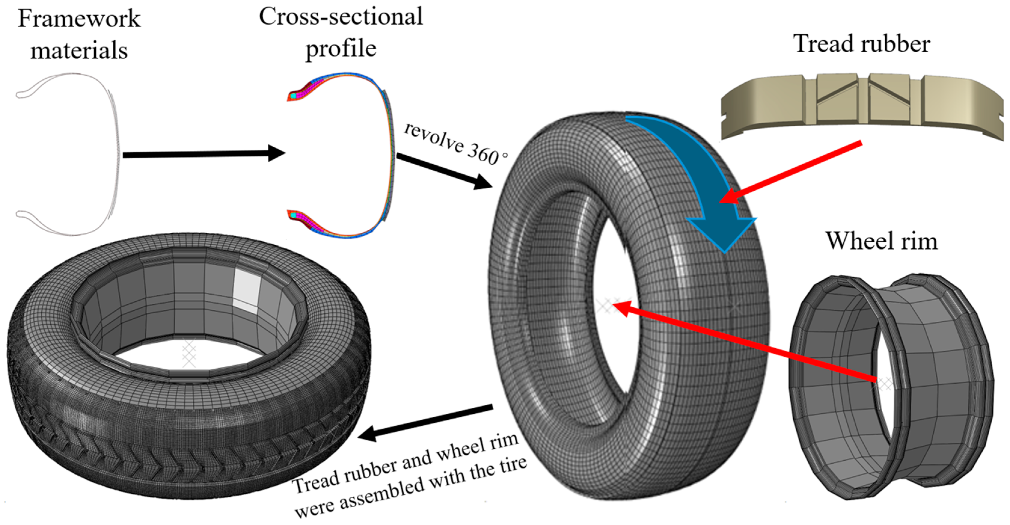
The tire model developed in this study was based on the Michelin ENERGY XM2+ (185/65R14), which is commonly used in passenger vehicles produced by Toyota, Honda, and Volkswagen. This radial tire consists of multiple materials and structural components. As a result, finite element modeling of the tire required the segmentation of different regions for independent meshing. This approach ensured that the constructed tire model exhibited physical properties identical to those of the real tire. Under vehicle weight load and hydrodynamic pressure during hydroplaning, the model reproduced deformation patterns consistent with the actual tire, serving as a prerequisite for ensuring the accuracy of hydroplaning simulations [25,26]. During the modeling process, the 2D cross-sectional profile of the tire was drawn in AutoCAD 2022 based on the actual dimensions of the tire model. Structural components such as the nylon overlay, belt, carcass ply, and inner liner, which served as the tire’s framework materials, were represented using lines. These lines were then imported into the meshing software HyperMesh 2019, where one-dimensional linear elements were used to model them. Independent surfaces corresponding to the sidewall, apex strip, rim cushion, bead wire, and bead filler were created over the framework. The two-dimensional tire structure with the framework was revolved 360° to form a basic tire model. Given that actual tires typically feature complex tread patterns composed mainly of transverse and longitudinal grooves, the tread rubber was modeled separately. The completed tread model was arrayed around the tire’s surface to create a detailed finite element tire model with structural characteristics identical to the real tire. The rim structure was bonded to the outer side of the tire using surface contact. A friction coefficient of 1.0 was applied to prevent relative displacement, effectively simulating the fixation of the tire to the rim in real-world conditions. This ensured that the tire experienced constraints identical to those of a real tire during motion. The modeling process is illustrated in Figure 1. This model accurately reflects the deformation of the tire under various working conditions, ensuring the precision of subsequent numerical simulation analyses.

Figure 1.
Tire model structure demonstration.
After establishing the tire model, it is necessary to set material parameters based on real material data. Tire rubber belongs to hyperelastic materials and the Yeoh model is often simulated in mechanical properties of hyperelastic materials [27]. The elastic strain energy function of the Yeoh model is depicted in Equation (1).
where and represent the material constants, as shown in Table 1. is the volumetric variation, and is the invariant of the Cauchy–Green deformation tensor. The deformation coefficient of the carcass material in Table 2 is measured using a universal testing machine [28].

Table 1.
Yeoh model parameters.
Table 2.
Elastic information parameters.
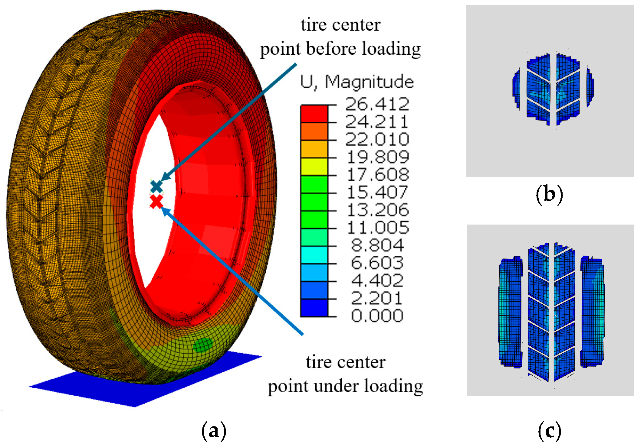
After assigning material parameters to the tire model, additional mechanical parameters were incorporated. To simulate the inflation pressure of a real tire, a uniformly distributed pressure of 0.24 MPa was applied to the inner surface of the tire. The road surface was modeled as a rigid flat plate with a friction coefficient of 0.8, which is consistent with the friction coefficient of an actual asphalt road. A vertical pressure of 3900 N is applied to the tire model to simulate the deformation caused by vehicle load (for a typical mid-size family car, such as a Honda Accord or Toyota Camry, weighing approximately 1400 kg to 1800 kg, we take an average value of 1600 kg; this weight is evenly distributed across four tires, resulting in each tire bearing a load of approximately 3900 N). The deformation contour of the tire under the combined effects of vehicle load, internal pressure, and ground support force is shown in Figure 2a. The blue cross represents the position of the tire’s center point before loading, while the red cross indicates its position after loading. It was observed that the center point of the tire moved downward under the applied load, with the tread region in contact with the ground flattening and the sidewall exhibiting bulging. This deformation occurred due to the redistribution of internal stress as the load was transmitted from the tire to the ground. Specifically, the contact area experienced compressive forces, while the sidewall region exhibited significant bulging caused by tensile forces. Figure 2b shows the tire’s contact area with the ground before loading, and Figure 2c illustrates the contact area after loading.

Figure 2.
Tire static load analysis by visualizing (a) the spatial displacement at nodes after tire loading, (b) the ground contact pressure at surface nodes of the tire before loading, and (c) the ground contact pressure at surface nodes of the tire under loading.
2.2. Setting Up the Hydroplaning Model
In previous studies, hydroplaning models were typically created by placing a rectangular component beneath the tire model and using Boolean operations to subtract overlapping regions, thereby extracting the fluid domain with the tire tread pattern [29,30]. The water inflow velocity at the inlet was set as equal in magnitude but opposite in direction to the vehicle’s speed. However, this method had a major limitation: it failed to allow fluid to enter the oblique grooves of the tire, resulting in an unrealistic representation of the hydroplaning process. This issue stemmed from the omission of the dynamic interaction between the rotating tire and the water surface. To overcome this limitation, a more advanced tire model was developed, incorporating both translational motion along the road surface and rotational motion around its central axis. By coupling the fluid domain with the tire and conducting fluid–structure interaction calculations, real-time interactions between the tire and the fluid were captured. This approach more accurately represented the iterative process between the tire’s deformation under load and the flow field variations within the fluid domain, providing a more realistic simulation of hydroplaning.
During the hydroplaning process, the tire is subjected not only to water’s viscous forces but also to the hydrodynamic pressure generated by water accumulating beneath the tire. In 1886, Reynolds introduced the fundamental equations of lubrication theory based on fluid mechanics, successfully uncovering the mechanism of hydrodynamic pressure generation in fluid films, which laid the foundation for modern fluid lubrication theory [31,32]. Before simulating the hydroplaning behavior, the tire and fluid domain were meshed using HyperMesh. To ensure the convergence of complex fluid–structure interaction (FSI) models, more than 99% of the meshes consisted of hexahedral elements. Each mesh element was treated as an infinitesimal unit, and the force equilibrium along the X-axis for these units was determined.
The infinitesimal fluid element is subjected only to the pressure exerted by adjacent fluid elements and the shear stress caused by fluid viscosity. represent the flow velocities in the X- and Y-axis directions, respectively. According to Newton’s law of viscosity , where the fluid is assumed to be Newtonian, and pressure variations in the thickness direction of the fluid film are neglected. By integrating the equation twice, the solution is obtained.
To determine the integration constants and , boundary conditions are applied. Since the fluid velocity at the interface equals the velocity of the surface, the velocities of the two solid surfaces are denoted as and , at , . At , , the equation is integrated along the thickness direction of the fluid film, resulting in the following expression:
By defining and , and introducing the relation , the simplified Reynolds equation is ultimately derived [33].
The simplified Reynolds equation effectively describes the flow behavior within the fluid domain. However, the presence of tire rotation introduces complexities into the fluid motion along the rotating wall surfaces. To address this, the volume of fluid (VOF) method is employed as a supplementary technique to enhance the numerical simulation of fluid flow through the tire tread pattern [34]. In the VOF method, the Eulerian volume fraction is defined based on the fluid passing through the computational grid, as shown in Equation (7). The function represents the ratio of the fluid volume within a Eulerian element to the total volume of that element and is a function of both space and time.
In the CEL method, if the element is fully filled with water, its volume fraction ; if no water is present in an element, then the volume fraction . In the hydroplaning simulation, both water and air voids are treated as Eulerian elements. If the sum of all material volume fractions in an element is less than one, then the volume fraction , and the air void will automatically fill the remainder of the element.
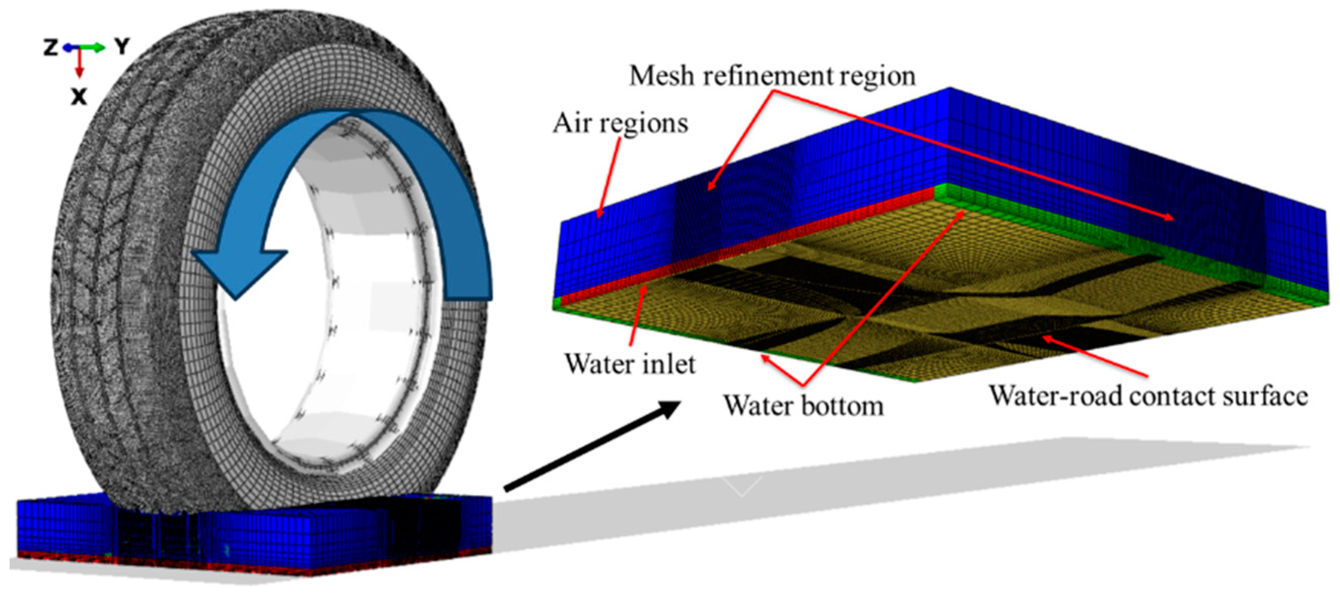
The entire fluid domain is composed of two parts. The bottom section, with a height of 7.684 mm, represents the fluid region simulating the water layer covering the road surface. The other section, with a height of 52.316 mm, represents the air domain. Both regions were established within the same fluid domain to simulate the scattering effect of water as the tire passes over the surface. The dimensions of the fluid domain were 60 mm in the x-axis direction, 390 mm in the y-axis direction, and 317 mm in the z-axis direction. Eulerian elements were used for the fluid model, with the element type defined as EC3D8R. The entire fluid model consisted of 415,576 nodes and 381,420 elements, as shown in Figure 3. Certain regions of the mesh appear darker in the figure due to mesh refinement in the areas critical for tire drainage. By reducing the mesh size in these regions by a factor of five, the simulation accuracy was further enhanced. The entire fluid domain was tied to the center point of the tire, ensuring that the fluid domain moved with the tire as it traveled across the road surface during the simulation. This eliminated the need to establish a fluid domain across the entire road, thereby reducing the total number of mesh elements and improving the computational efficiency of the numerical simulation.

Figure 3.
Whole tire hydroplaning model, comprising tire, fluid, and ground considerations.
3. Simulation and Validation of the Tire Hydroplaning Model
3.1. Tire Hydroplaning
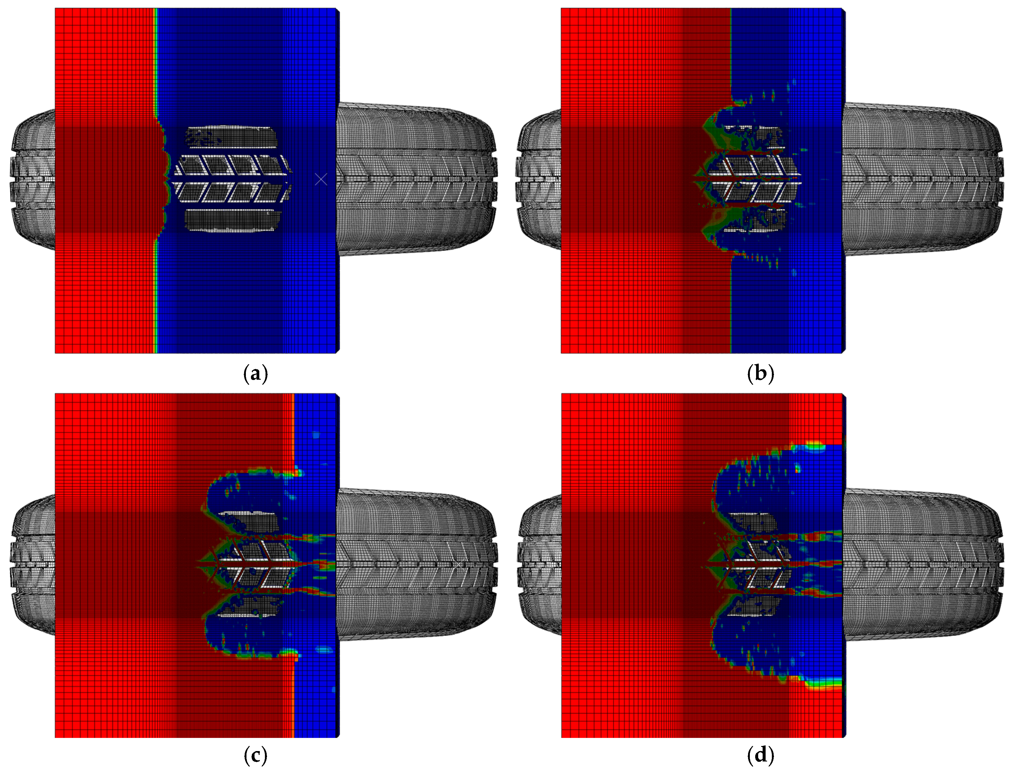
A simulation was conducted on a 185/65R14 tire under the conditions of an inflation pressure of 240 kPa and a fluid surface height of 7.684 mm, with the tire traveling at a speed of 70 km/h. As shown in the contour plots in Figure 3, at 7.00533 s of simulation time, the tire had just made initial contact with the water. At this stage, insufficient hydrodynamic pressure had developed, and the tire’s drainage performance was negligible. Consequently, the tire’s contact area with the ground was at its maximum, and the ground contact stress reached its peak, as shown in Figure 4a. At 7.00933 s, the tire was fully in contact with the water, and fluid had begun entering the tire grooves. During this phase, the hydrodynamic pressure started to increase gradually, as shown in Figure 4b. By 7.01333 s, the appearance of more red regions in the grooves indicated that the drainage performance of the tire grooves was becoming more evident. The grooves began to significantly influence the tire’s ability to displace water. The contact area with the ground further decreased, suggesting a reduction in the ground contact stress, as shown in Figure 4c. Compared to the conditions at 7.00533 s, the contact area between the tire and the ground had diminished, as shown in the contour plots. However, since the tire had not yet fully transitioned to a water-covered road, water displacement from the ground contact region was primarily achieved through the grooves and tire’s sides. At 7.02133 s, the tire was in full contact with the fluid, and the curvature of water displacement to both sides of the tire became significantly more pronounced, as shown in Figure 4d.

Figure 4.
Tire hydroplaning process: (a) time = 7.00533 s; (b) time = 7.00933 s; (c) time = 7.01333 s; (d) time = 7.02133 s.
3.2. Validation of the Fluid–Structure Coupling Model
The introduction reviewed extensive research conducted by domestic and international scholars in the field of tire hydroplaning. Most of these studies highlighted the widely recognized NASA hydroplaning empirical formula, which has been broadly acknowledged for its accuracy in the tire and transportation industries [35,36,37]. In this study, a comparison was made between a tire hydroplaning model and the NASA hydroplaning empirical formula. The hydroplaning speed of the tire was determined under conditions where the inflation pressure gradually increased from 100 kPa to 250 kPa, with the radial pressure between the road surface and the tire set to zero. The NASA hydroplaning empirical formula is as follows:
where, is the hydroplaning speed in km/h and is the inflation pressure in .
A comparison was conducted between the simulation results obtained from the developed model and the critical hydroplaning speeds calculated using the NASA empirical formula. At an inflation pressure of 100 kPa, the NASA formula predicted a critical hydroplaning speed of 64.3 km/h, while the model produced a value of 71 km/h, resulting in a 9% error. When the inflation pressure increased to 140 kPa, the NASA formula calculated a speed of 76 km/h, compared to 75 km/h from the model, with an error of 1.3%. At 150 kPa, the NASA formula predicted a speed of 86.3 km/h, whereas the model yielded a result of 78 km/h, with a 10% error. The differences between the two curves arise from variations in the tire hardness and tread pattern used in the numerical simulation compared to those in the NASA experiments. These differences influence the tire deformation and tread drainage performance, leading to inevitable discrepancies between the simulation results and the empirical formula predictions.
4. Effects of Various Environmental Conditions on Tire Hydroplaning
4.1. Under the Conditions of Different Road Water Depths
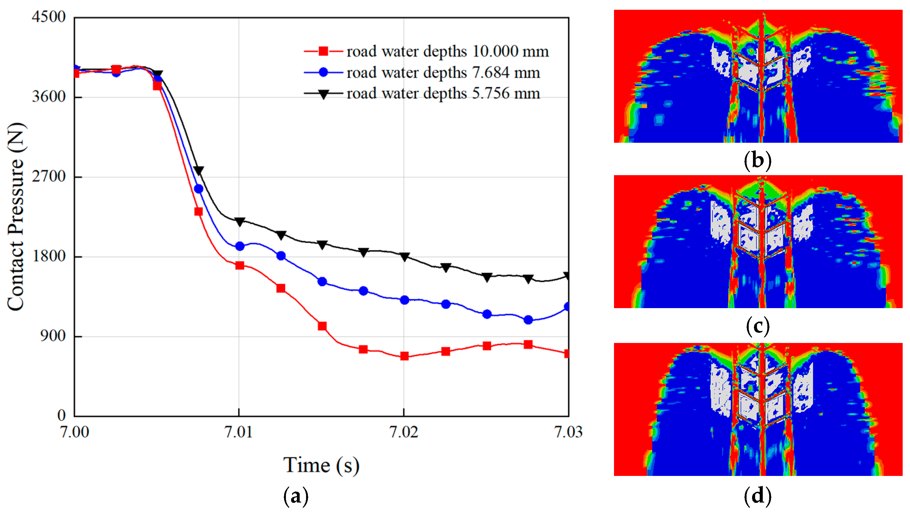
The radial ground pressure of the tire discussed earlier corresponded to the water depth of 7.684 mm. When the depth of water on the road surface changed, the radial vertical load between the tire and the ground varied, as shown in Figure 5a. The figure reveals that as the water film thickness increased, the contact pressure between the tire and the ground decreased. The variation of the three curves in the figure indicates that thicker water films caused a greater reduction in the vertical contact force of the tire. This phenomenon occurred because deeper water on the road accumulated more water at the leading edge of the tire, while the limited space between the tire and the ground resulted in higher hydrodynamic pressure [38]. When the water depth was 5.756 mm, the tire-to-ground contact pressure was at its maximum, and Figure 5d shows that the tire-to-ground contact area was also at its largest at this point. Conversely, when the water depth reached 10.000 mm, the contact pressure was at its minimum, as Figure 5b demonstrates, with the smallest contact area. These findings indicate that as the road water depth increased, the contact pressure between the tire and the ground decreased while the hydrodynamic pressure rose. With increasing water depth, the hydrodynamic pressure gradually lifted the tire, reducing the ground contact and significantly increasing the risk of hydroplaning.
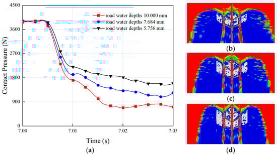
Figure 5.
Effect of water depth on tire hydroplaning: (a) contact pressure during hydroplaning for tires at different water depths. The ground contact areas of (b) water = 10.000 mm; (c) water = 7.684 mm; (d) water = 5.756 mm.
Additionally, by comparing the fluctuations of the three curves, it was observed that shallower water depths resulted in smoother curves with smaller fluctuations. These fluctuations corresponded to variations in the contact pressure during hydroplaning. This indicates that deeper water on the road led to faster force changes during driving, making vehicle control more difficult and further elevating the hydroplaning risk. This aspect of rapid force variation with deeper water, and its impact on vehicle control has been previously overlooked in hydroplaning studies.
4.2. Under the Conditions of Different Driving Speeds
The driving speed of a vehicle directly influences the hydroplaning resistance of tires on wet surfaces [39]. High speeds reduce the contact time between the tire and the road, making it more difficult for the tire to adapt to surface irregularities and wet conditions, thereby decreasing traction. On wet roads, tires require additional time to expel water, but high speeds limit this process, leading to a loss of effective adhesion between the tire and the road. The simulation results of the relationship between vehicle speed and the radial vertical contact pressure of the tire are presented in Figure 6a. The figure shows that as the vehicle speed increased, the radial vertical contact pressure of the tire decreased. Corresponding to Figure 6d,e, the contact area between the tire and the road progressively diminished. At a speed of 81 km/h, the contact pressure between the tire and the road dropped to zero, as illustrated in Figure 6c, where the tire completely lost contact with the ground. This indicates that 81 km/h was the critical hydroplaning speed for the tire. When the vehicle speed further increased to 85 km/h, the rate of decrease in the tire-to-ground contact pressure accelerated, making it more likely for the tire to lose contact with the road entirely. Therefore, to ensure travel safety, the vehicle speed should not exceed the tire’s critical hydroplaning speed. Once this speed is surpassed, the tire completely loses contact with the road, resulting in the loss of vehicle control and an increased risk of traffic accidents.
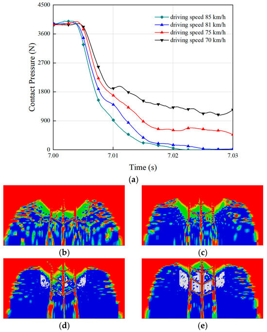
Figure 6.
Effect of driving speed on tire hydroplaning: (a) the contact pressure with the ground during hydroplaning for tires at different driving speeds. The ground contact areas of (b) speed = 85 km/h; (c) speed = 81 km/h; (d) speed = 75 km/h; (e) speed = 70 km/h.
4.3. Under the Conditions of Different Tire Loads
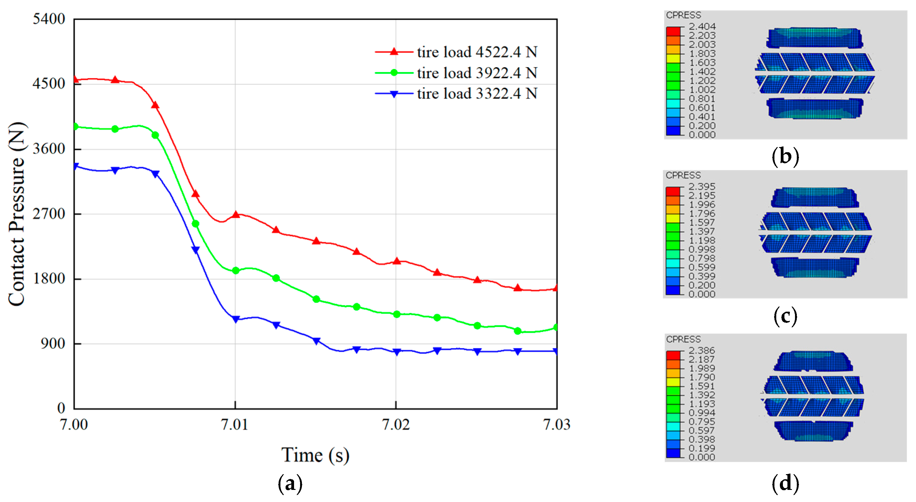
The tire load, referring to the vertical force exerted on the tire, represents the force transmitted from the vehicle to the ground through the tire. The tire load significantly influences hydroplaning performance, with the most evident effect being that an increase in tire load generally enhances the contact pressure between the tire and the ground, thereby improving grip [40]. A greater vertical load increases the contact area between the tire tread and the road surface, enabling better traction and thus enhancing hydroplaning resistance. Moderate tire loads can improve vehicle handling, as increased vertical loads contribute to vehicle stability and enhance cornering grip. The influence of the tire load on hydroplaning performance is primarily reflected in changes in the ground contact pressure. Variations in the tire contact pressure under different loads during hydroplaning are shown in Figure 7a. As illustrated, the initial contact pressure between the tire and the ground differs under varying loads. An increase in load improves the contact pressure between the tire and the ground during hydroplaning. For example, when the load increased from 2922.4 N to 3322.4 N, the tire’s contact force with the ground during hydroplaning rose by 200 N. Further increasing the load from 3322.4 N to 4522.4 N resulted in a contact force increase of 600 N. Hence, increasing tire load effectively mitigates hydroplaning, with larger weight increments producing more significant improvements in hydroplaning resistance. Comparing Figure 7b,d reveals that increasing the load also enlarges the tire–road contact area due to the deformation of the tire under stress. Overall, increasing tire load enhances the contact area and pressure between the tire and the ground, making it an effective strategy for improving hydroplaning resistance.
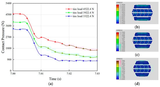
Figure 7.
Effect of load on tire hydroplaning: (a) the contact pressure with the ground during hydroplaning of tires under different loads. The contact pressure at surface nodes under loads of (b) 4522.4 N; (c) 3922.4 N; (d) 3322.4 N.
4.4. Under the Conditions of Different Inflation Pressures
The inflation pressure of a tire significantly influences its hydroplaning performance by directly affecting the contact area between the tire and the ground [41]. A proper inflation pressure ensures uniform tread contact with the road surface, thereby enhancing grip. The effect of inflation pressure on hydroplaning performance is illustrated in Figure 8a. Analyzing the curves in the figure reveals that the contact pressure between the tire and the ground showed minimal variation when the inflation pressures were 0.24 MPa and 0.34 MPa. This is because at these inflation pressures, the deformation of the tire sidewall was relatively minor, as shown in Figure 8b,c, resulting in limited impact on the tire’s drainage performance. Consequently, with negligible changes in hydrodynamic pressure, the contact pressure remained the same. However, at an inflation pressure of 0.14 MPa, the tire sidewall exhibited significant deformation, reducing the distance between the tire center and the ground and narrowing the gap between the tire and the surface, as depicted in Figure 8d. By contrast, a tire with an inflation pressure of 0.34 MPa created a larger gap between the tire and the ground, which was more conducive to water evacuation along the sides of the tire. This reduced water accumulation between the tire and the ground decreases the hydrodynamic pressure and increases the contact pressure. Maintaining appropriate inflation pressure not only improves driving safety but also extends the tire lifespan. Drivers are advised to regularly check the tire inflation pressure and ensure that it remains within the manufacturer’s recommended range.
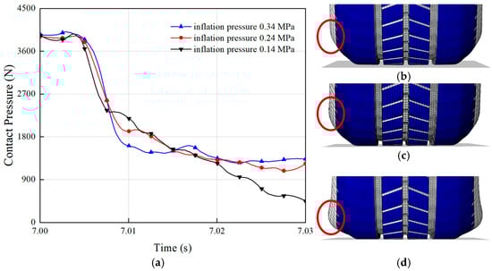
Figure 8.
Effect of inflation pressure on tire hydroplaning: (a) the contact pressure with the ground during hydroplaning for two types of tires at different inflation pressures. The sidewall deformation at inflation pressures of (b) 0.34 MPa; (c) 0.24 MPa; (d) 0.14 MPa.
5. Conclusions
This study selected a 185/65R14 radial tire as the prototype to conduct an in-depth analysis of the hydroplaning phenomenon. The effects of external factors, such as the water depth, vehicle speed, tire load, and inflation pressure, on the tire’s hydroplaning resistance were analyzed. It was found that the water depth influences the hydroplaning performance in two ways. First, as the water depth increases, the tire’s contact area and pressure with the ground decreases, reducing stability during rotation and impairing hydroplaning resistance. Second, higher driving speeds increase the likelihood of hydroplaning, as excessive speed reduces the time available for water evacuation, resulting in greater water accumulation between the tire and the road surface. In emergency situations requiring high-speed driving, increasing the vehicle load or tire inflation pressure could improve hydroplaning resistance. A higher load directly increases the tire’s contact pressure with the ground, while a higher inflation pressure expands the drainage space on both sides of the tire, effectively reducing the water accumulation and fluid dynamic pressure between the tire and road surface, thus enhancing hydroplaning resistance. With the rapid advancements in autonomous driving and intelligent tire technologies, this comprehensive investigation into hydroplaning performance provides a theoretical foundation for optimizing sensors, intelligent tire pressure adjustment systems, and active safety technologies, facilitating their real-world application.
Author Contributions
Conceptualization, T.D. and L.Z.; methodology, T.D.; software, D.C.; validation, S.W.; formal analysis, T.D.; investigation, S.W.; resources, D.C.; data curation, T.D.; writing—original draft preparation, T.D.; writing—review and editing, L.Z.; supervision, L.R.; project administration, L.Z. All authors have read and agreed to the published version of the manuscript.
Funding
This work was supported by the Key Research Project of Shandong Provincial Natural Science Foundation (ZR2021ZD27) and the Open Project Program of the Key Laboratory for Cross-Scale Micro and Nano Manufacturing, Ministry of Education, Changchun University of Science and Technology (CMNM-KF202103).
Data Availability Statement
The raw data supporting the conclusions of this article will be made available by the authors on request.
Acknowledgments
The authors acknowledge support from the Weihai Bionics Research Institute—Jilin University.
Conflicts of Interest
Author Dichuan Cheng was employed by the company EVE Energy Co., Ltd. The remaining authors declare that the research was conducted in the absence of any commercial or financial relationships that could be construed as a potential conflict of interest.
References
- Murad, M.M.; Abaza, K.A. Pavement Friction in a Program to Reduce Wet Weather Traffic Accidents at the Network Level. Transp. Res. Record 2006, 1949, 126–136. [Google Scholar] [CrossRef]
- Schmid, F.; Lohner, T.; Stahl, K. Friction in Oil-Lubricated Rolling–Sliding Contacts with Technical and High-Performance Thermoplastics. Lubricants 2024, 12, 372. [Google Scholar] [CrossRef]
- Liang, X.; Han, M.; He, T.; Cui, L.; Yang, Z.; Ouyang, W. A Mixed Lubrication Deterministic Model of an Elastic Support Water-Lubricated Tilting Pad Thrust Bearing. Lubricants 2023, 11, 262. [Google Scholar] [CrossRef]
- Ding, Y.M.; Wang, H. Computational investigation of hydroplaning risk of wide-base truck tyres on roadway. Int. J. Pavement Eng. 2020, 21, 122–133. [Google Scholar] [CrossRef]
- Hermange, C.; Oger, G.; Le Chenadec, Y.; Le Touzé, D. A 3D SPH–FE coupling for FSI problems and its application to tire hydroplaning simulations on rough ground. Comput. Meth. Appl. Mech. Eng. 2019, 355, 558–590. [Google Scholar] [CrossRef]
- Hermange, C.; Oger, G.; Le Chenadec, Y.; de Leffe, M.; Le Touzé, D. In-depth analysis of hydroplaning phenomenon accounting for tire wear on smooth ground. J. Fluids Struct. 2022, 111, 103555. [Google Scholar] [CrossRef]
- Spitzhuttl, F.; Goizet, F.; Unger, T.; Biesse, F. The real impact of full hydroplaning on driving safety. Accid. Anal. Prev. 2020, 138, 105458. [Google Scholar] [CrossRef]
- Hermange, C.; Todoroff, V.; Biesse, F.; Le-Chenadec, Y. Experimental investigation of the leading parameters influencing the hydroplaning phenomenon. Veh. Syst. Dyn. 2021, 60, 2375–2392. [Google Scholar] [CrossRef]
- Dreher, R.C.; Horne, W.B. Phenomena of Pneumatic Tire Hydroplaning. 1963. Available online: https://ntrs.nasa.gov/citations/19640000612 (accessed on 20 October 2024).
- Dehnad, M.H.; Khodaii, A. Evaluating the effect of different asphalt mixtures on hydroplaning using a new lab-scale apparatus. Pet. Sci. Technol. 2016, 34, 1726–1733. [Google Scholar] [CrossRef]
- Srirangam, S.K.; Anupam, K.; Scarpas, A.; Kasbergen, C.; Kane, M. Safety Aspects of Wet Asphalt Pavement Surfaces through Field and Numerical Modeling Investigations. Transp. Res. Record 2014, 2446, 37–51. [Google Scholar] [CrossRef]
- Zheng, B.; Huang, X.; Zhang, W.; Zhao, R.; Zhu, S. Adhesion characteristics of tire-asphalt pavement interface based on a proposed tire hydroplaning model. Adv. Mater. Sci. Eng. 2018, 2018, 5916180. [Google Scholar] [CrossRef]
- Suzuki, T.; Fujikawa, T. Improvement of Hydroplaning Performance Based on Water Flow around Tires. SAE Trans. 2001, 110, 830–835. [Google Scholar] [CrossRef]
- Zhou, H.; Jiang, Z.; Jiang, B.; Wang, H.; Wang, G.; Qian, H. Optimization of tire tread pattern based on flow characteristics to improve hydroplaning resistance. Proc. Inst. Mech. Eng. Part D-J. Automob. Eng. 2020, 234, 2961–2974. [Google Scholar] [CrossRef]
- Löwer, J.; Wagner, P.; Unrau, H.J.; Bederna, C.; Gauterin, F. Dynamic measurement of the fluid pressure in the tire contact area on wet roads. Automot. Engine Technol. 2020, 5, 29–36. [Google Scholar] [CrossRef]
- Allbert, B.J. Tires and Hydroplaning. SAE Trans. 1968, 77, 593–603. Available online: https://www.jstor.org/stable/44565087 (accessed on 20 October 2024).
- Ong, G.P.; Fwa, T.F. Wet-Pavement Hydroplaning Risk and Skid Resistance: Modeling. J. Transp. Eng. 2007, 133, 590–598. [Google Scholar] [CrossRef]
- Ong, G.P.; Fwa, T.F. Mechanistic Interpretation of Braking Distance Specifications and Pavement Friction Requirements. Transp. Res. Record 2010, 2155, 145–157. [Google Scholar] [CrossRef]
- Cho, J.; Lee, H.; Sohn, J.; Kim, G.; Woo, J. Numerical investigation of hydroplaning characteristics of three-dimensional patterned tire. Eur. J. Mech. A Solids 2006, 25, 914–926. [Google Scholar] [CrossRef]
- Wies, B.; Roeger, B.; Mundl, R. Influence of Pattern Void on Hydroplaning and Related Target Conflicts. Tire Sci. Technol. 2009, 37, 187–206. [Google Scholar] [CrossRef]
- El-Sayegh, Z.; El-Gindy, M.; Johansson, I.; Oijer, F. Modeling of Tire-Wet Surface Interaction Using Finite Element Analysis and Smoothed-Particle Hydrodynamics Techniques; SAE Technical Paper 2018-01-1118; SAE: Warrendale, PA, USA, 2018. [Google Scholar] [CrossRef]
- Kumar, S.S.; Anupam, K.; Scarpas, T.; Kasbergen, C. Study of Hydroplaning Risk on Rolling and Sliding Passenger Car. Procedia Soc. Behav. Sci. 2012, 53, 1019–1027. [Google Scholar] [CrossRef]
- Baranowski, P.; Małachowski, J.; Mazurkiewicz, Ł. Local blast wave interaction with tire structure. Def. Technol. 2020, 16, 520–529. [Google Scholar] [CrossRef]
- Liang, C.; Gao, Z.; Hong, S.; Wang, G.; Kwaku Asafo-Duho, B.M.; Ren, J.; Palumbo, D. A Fatigue Evaluation Method for Radial Tire Based on Strain Energy Density Gradient. Adv. Mater. Sci. Eng. 2021, 2021, 85349542. [Google Scholar] [CrossRef]
- Ge, Y.; Yan, Y.; Yan, X.; Meng, Z. Study on Static Stiffness Characteristics and Influencing Factors of Radial Pneumatic Tire with Complex Tread Patterns by Computer Simulation Method. In Proceedings of the 2022 2nd International Conference on Computational Modeling, Simulation and Data Analysis (CMSDA), Zhuhai, China, 2–4 December 2022; pp. 1–6. [Google Scholar] [CrossRef]
- Liu, Q.; Pei, J.; Wang, Z.; Hu, D.; Huang, G.; Meng, Y.; Lyu, L.; Zheng, F. Analysis of tire-pavement interaction modeling and rolling energy consumption based on finite element simulation. Constr. Build Mater. 2024, 425, 136101. [Google Scholar] [CrossRef]
- Benevides, R.O.; Nunes, L.C.S. Mechanical behavior of the alumina-filled silicone rubber under pure shear at finite strain. Mech. Mater. 2015, 85, 57–65. [Google Scholar] [CrossRef]
- Goodchild, I.R.; Muhr, A.H.; Thomas, A.G. The lateral stiffness and damping of a stretched rubber beam. Plast. Rubber Compos. 2018, 47, 176–186. [Google Scholar] [CrossRef]
- Zhang, L.; Fwa, T.F.; Ong, G.P.; Chu, L. Analysing effect of roadway width on skid resistance of porous pavement. Road Mater. Pavement Des. 2015, 17, 1–14. [Google Scholar] [CrossRef]
- Pasindu, H.R.; Fwa, T.F.; Ong, G.P. Analytical evaluation of aircraft operational risks from runway rutting. Int. J. Pavement Eng. 2015, 17, 810–817. [Google Scholar] [CrossRef]
- Georgescu, A.; Nicolescu, B.; Popa, N.; Boloşteanu, M. On special solutions of the Reynolds equation from lubrication. J. Comput. Appl. Math. 2001, 133, 367–372. [Google Scholar] [CrossRef]
- Goyon, O. High-Reynolds number solutions of Navier-Stokes equations using incremental unknowns. Comput. Meth. Appl. Mech. Eng. 1996, 130, 319–335. [Google Scholar] [CrossRef]
- Dowson, D. A generalized Reynolds equation for fluid-film lubrication. Int. J. Mech. Sci. 1962, 4, 159–170. [Google Scholar] [CrossRef]
- Cho, J.R.; Lee, S.Y. Dynamic analysis of baffled fuel-storage tanks using the ALE finite element method. Int. J. Numer. Methods Fluids 2003, 41, 185–208. [Google Scholar] [CrossRef]
- Wang, N.; Chu, L.; Fwa, T.F. Improved method for evaluation of effect of pavement microtexture on vehicle hydroplaning speed. Constr. Build. Mater. 2024, 451, 138727. [Google Scholar] [CrossRef]
- Dehnad, M.H.; Yazdi, A. A review of numerical and experimental studies on hydroplaning of vehicles in motion on road surfaces. Results Eng. 2024, 23, 102438. [Google Scholar] [CrossRef]
- Fwa, T.F. Pavement skid resistance properties for safe aircraft operations. J. Road. Eng. 2024, 4, 361–385. [Google Scholar] [CrossRef]
- Cerezo, V.; Gothié, M.; Menissier, M.; Gibrat, T. Hydroplaning speed and infrastructure characteristics. Proc. Inst. Mech. Eng. Part J J. Eng. Tribol. 2010, 224, 891–898. [Google Scholar] [CrossRef]
- Chen, X.; Wang, H. Analysis and mitigation of hydroplaning risk considering spatial-temporal water condition on the pavement surface. Int. J. Pavement Eng. 2023, 24, 2036988. [Google Scholar] [CrossRef]
- Meethum, P.; Suvanjumrat, C. Hydroplaning Effects of Tread Patterns of Motorcycle Tires. J. Transp. Eng. Part B Pavements 2025, 151, 04024052. [Google Scholar] [CrossRef]
- Chaiworapuek, W.; Suvanjumrat, C.; Worajinda, N.; Rugsaj, R. Development of contact area model for motorcycle tire hydroplaning through experimental investigation. Int. J. GEOMATE 2024, 26, 66–73. [Google Scholar] [CrossRef]


Disclaimer/Publisher’s Note: The statements, opinions and data contained in all publications are solely those of the individual author(s) and contributor(s) and not of MDPI and/or the editor(s). MDPI and/or the editor(s) disclaim responsibility for any injury to people or property resulting from any ideas, methods, instructions or products referred to in the content. |
© 2025 by the authors. Licensee MDPI, Basel, Switzerland. This article is an open access article distributed under the terms and conditions of the Creative Commons Attribution (CC BY) license (https://creativecommons.org/licenses/by/4.0/).