Article

Inertial and Linear Re-Absorption Effects on a Synovial Fluid Flow Through a Lubricated Knee Joint

1
Department of Mathematics, Pennsylvania State University, York Campus, 1031 Edgecomb Avenue, York, PA 17403, USA
2
Department of Mathematics & Statistics, International Islamic University, Islamabad 44000, Pakistan
3
Department of Mathematical Sciences, Federal Urdu University of Arts, Sciences & Technology, Islamabad 44000, Pakistan
*
Author to whom correspondence should be addressed.
Lubricants 2025, 13(5), 196; https://doi.org/10.3390/lubricants13050196
Submission received: 14 February 2025 / Revised: 15 April 2025 / Accepted: 22 April 2025 / Published: 27 April 2025

Abstract

:
This study examines the flow dynamics of synovial fluid within a lubricated knee joint during movement, incorporating the effect of inertia and linear re-absorption at the synovial membrane. The fluid behavior is modeled using a couple-stress fluid framework, which accounts for mechanical phenomena and employs a lubricated membrane. synovial membrane plays a crucial role in reducing drag and enhancing joint lubrication for the formation of a uniform lubrication layer over the cartilage surfaces. The mathematical model of synovial fluid flow through the knee joint presents a set of non-linear partial differential equations solved by a recursive approach and inverse method through the software Mathematica 11. The results indicate that synovial fluid flow generates high pressure and shear stress away from the entry point due to the combined effects of inertial forces, linear re-absorption, and micro-rotation within the couple-stress fluid. Axial flow intensifies at the center of the knee joint during activity in the presence of linear re-absorption and molecular rotation, while transverse flow increases away from the center and near to synovium due to its permeability. These findings provide critical insights for biomedical engineers to quantify pressure and stress distributions in synovial fluid to design artificial joints.

1. Introduction

This research aims to analyze the flow of synovial fluid (SF) through the synovium in the knee joint. SF plays a crucial role in joint lubrication, reducing cartilage friction for smooth movement. It is located near the synovial membrane (SM), which consists of collagens, proteins, and proteoglycans—key components influencing SF viscosity. The selectively permeable SM allows the absorption and secretion of SF, regulating water balance to prevent joint swelling (effusion) or inadequate lubrication, which may lead to joint damage.
Several studies have examined SF flow characteristics. Yin et al. [1] highlighted the complexity of SF as a filtrate of interstitial fluids. Lai et al. [2] noted that SF flow depends on shear stress and deformation rate, but no single fluid model accurately describes its rheology. Ouerfelli et al. [3] emphasized the role of hyaluronic acid (HA) in joint lubrication, where SF behaves as a non-Newtonian fluid, shifting to Newtonian behavior after hyaluronidase treatment in osteoarthritis. Singh et al. [4] explored SF analysis for arthritis treatment, while Hasnain et al. [5] modeled SF as a power-law fluid incorporating permeability and magnetic field effects. Maqbool et al. [6,7] analyzed SF flow through permeable conduits using the Linear Phan-Thien-Tanner (LPTT) model and found that periodic filtration influences pressure and velocity distribution. The viscosity of SF is determined by HA molecular size and concentration, and its long-chain molecules can be modeled as a polar fluid. Rumanian et al. [8,9] used the couple-stress fluid model to study the hydrodynamic lubrication, noting the presence of couple stresses in fluids with large molecular structures. Previous studies [10,11,12,13,14,15] analyzed couple-stress effects in various flow conditions but did not consider SF as a couple-stress fluid.
Inertial (non-creeping) flow occurs at high shear rates during activities like running and jumping, which facilitates nutrient exchange and fluid circulation in the joint. For the healthy synovial fluid properties and consistent joint motion, nutrient re-absorption in synovial fluid follows the linear trajectory. This linear behavior is typically observed in a well-lubricated joint environment where the biomechanical load and fluid dynamics are favorable. Several researchers [16,17,18,19,20,21,22] have examined the impact of exercise on SF composition and joint performance. Oates [23] observed inertial forces in sudden joint movements, while Mow [24] explored bio-mechanical factors affecting joint health. Hron et al. [25] and Ruggior [26] studied inertial effects on SF flow in one dimension, but no one has examined it in a two-dimensional rectangular permeable synovium under slip and linear re-absorption effect, which is the novelty of this study.
This research uniquely analyzes SF as a couple-stress fluid under inertial effects through a permeable membrane with linear re-absorption. Unlike prior studies that primarily considered creeping flows and ignored membrane permeability, this research has considered the ignored inertial and linear re-absorption effects. The mathematical model is computed by employing a recursive and inverse approach to find the flow properties under constant flux at the entrance. The findings will assist biomedical engineers in calculating SF forces and flow properties under dynamic conditions which are essential for designing the artificial joint and surgical techniques.
The research is structured as follows: Section 1 reviews the literature and identifies research gaps, Section 2 models SF flow using mechanical laws and applies recursive approach and inverse methods to solve the problem, Section 3 presents graphical results for flow speed, load, and shear stress, and Section 4 concludes the study.

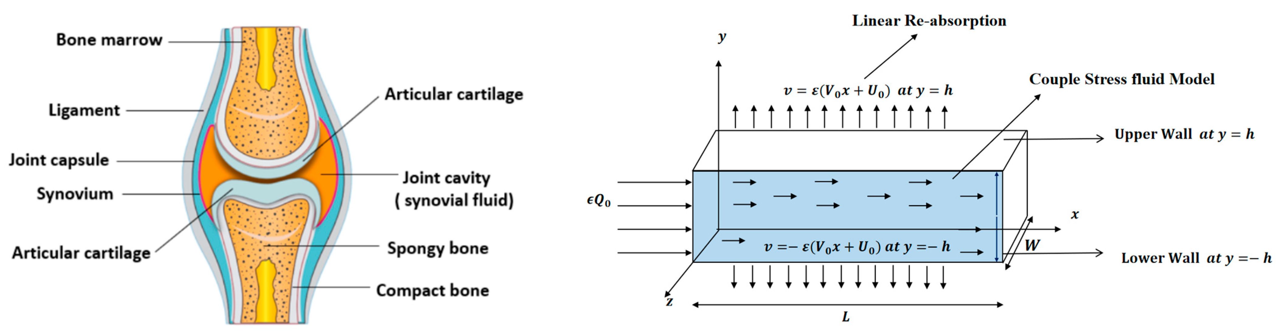
2. Materials and Methods

During joint movement, synovial fluid experiences both rotational and shear movement, which cannot be described by a simple model of non-Newtonian fluid. The couple stress fluid model has the ability to describe the shear and rotational motion. Micro-rotational effects lead to the assumption that the couple-stress fluid is a synovial fluid because synovial fluid not only lubricates but also provides aid to transfer forces (shear and rotational) within the joint. The scientific model of synovial fluid flow via a knee joint in the absence of roughness of surface considers planar geometry of two-dimensional cross-sectional area of a slit as given in Figure 1 filled with synovial fluid and the permeable wall of the slit resembles the synovial membrane. It is also assumed height h is lesser than the length L and width W is very small as compare to the height of slit, i.e., W < < h < L , it is mentioned in the geometry that length L is along the x -axis, width W is along the z -axis, and height h is along the y -axis. Flow is considered to be symmetric about the center line at y = 0 , i.e fluid flow in the upper region of the slit ( 0 < y < h ) , the lower region of slit ( h < y < 0 ) has the same behavior, and the rate at which nutrients and liquids in the synovial fluid are reabsorbed is not constant and linear due to the fast movement of fluid particles in the presence of inertial forces and non-porous medium.
The movement of synovial fluid in the knee joint suggests the following velocity field:
V = u ( x , y ) , v ( x , y ) , 0 ,
where u ( x , y ) and v ( x , y ) are flow velocity along and across the slit, respectively.
The synovial fluid flow can be described by the following continuity equation for in-compressible flow and the momentum equation for the steady couple stress fluid flow:
V = 0 ,  
ρ V t + V V = p + µ 2 V µ 1 4 V .
where 4 = 22, p is the hydrostatic pressure of the fluid, μ is the dynamic viscosity of the fluid, and μ 1 is the material constant associated with couple-stress fluid.
The slip velocity and linear re-absorption rate at the synovial membrane suggest the following conditions:
u = ± β u y ,   v = ± ε V 0 x + U 0 ,   a t   y = ± h ,
where 0 < β 1 is the slip parameter V 0 and U 0   are re-absorption velocity parameters.
The change in velocity gradient at walls suggests the following condition:
  2 u y 2 = 0 ,       a t   y = ± h ,
The synovial fluid enters in the flow regime with a constant flow rate and satisfies the following condition at the entry point x = 0.
ε Q 0 = 2 W 0 h u d y ,         a t   x = 0 .
where Q 0 is the volumetric flow rate at the entrance region, defining the inlet condition, and ε is the small parameter.
For two-dimensional steady-state inertial flow, the component form of the continuity and momentum equations are as follows:
u x + u y = 0 ,
ρ u u x + v v y = p x + µ 2 u µ 1 4 u ,
  ρ u u x + v v y = p y + µ 2 v µ 1 4 v .

2.1. Non-Dimensional Quantities

The non-dimensional quantities are defined as follows:
x = x L   y = y h   u = h 2 u Q 0   v = v h L Q 0   p = p h 4 μ L Q 0   δ = h L   R e = ρ Q 0 μ h ,     α = μ μ 1 .
Using the above quantities in Equations (7)–(9), and ignoring primes, one can write the following equations:
u x + u y = 0 ,
δ R e V u = p x + N 1 N 2 ,  
  δ 3 R e V v = p y + N 3 N 4 ,  
where
N 1 = δ 2 2 u x 2 + 2 u y 2 ,   N 2 = 1 α 2 δ 4 4 u x 4 + 4 u y 4 + δ 2 2 4 u x 2 y 2 ,
N 3 = δ 4 2 v x 2 + δ 2 2 v y 2 ,   N 4 = 1 α 2 δ 6 4 v x 4 + δ 2 4 v y 4 + δ 4 2 4 v x 2 y 2 ,
The dimensionless form of the boundary conditions will take the following form:
u = ± β u y ,   v = ± ε V 0 x + U 0 ,   a t   y = ± 1 ,  
2 u y 2 = 0 ,       a t   y = ± 1 ,  
ε = 2 A 0 1 u d y ,         a t   x = 0 .
where A = W h .

2.2. Solution Methodology

The mathematical model given in Equations (11)–(13) will help to determine the formulas for flow rate, normal and tangential forces in synovial fluid. The mathematical model of non-linear partial differential equations in u ,   v   a n d   p   reduces into simple form under the assumption that the length of synovial membrane (slit) is smaller than its width. After using the assumption that the ratio of length to width ( δ ) is very small the higher-order terms like δ 2 ,   δ 3 ,   a n d   δ 4   will be ignored from Equations (12) and (13).
To find the results for u, v ,   a n d   p ,   the following recursive approach is used:
u = l i m ε 1 i = 1 ε i u ( i )   ,   v = l i m ε 1   i = 1 ε i v ( i ) ,   p = p ( 0 ) + l i m ε 1 i = 1 ε i p ( i ) .  
where p ( 0 ) is a constant.
Now by substituting above mention series in Equations (11)–(16) and then by collecting powers of ε , one can obtain the following systems:

2.2.1. First Order System and Its Solution

The solution of following first order system can be obtained by inverse method which is calculated in this section:
u 1 x + u 1 y = 0 ,  
0 = p 1 x + 2 u 1 y 2 1 α 2   4 u 1 y 4 ,
0 =   p 1 y ,
The associated boundary conditions for a first-order system are defined as follows:
u ( 1 ) = ± β u ( 1 ) y ,         v ( 1 ) = ± ( V 0 x + U 0 ) ,         a t   y = ± 1 ,
2 u 1 y 2 = 0 ,   a t   y = ± 1 ,
h = 2 W 0 1 u ( 1 ) d y ,         a t   x = 0 .  
To reduce the number of unknowns, one can introduce the following stream function ψ 1 x , y :
  u 1 = ψ ( 1 ) y ,     v 1 = ψ 1 x ,
After replacing u 1 and v 1 in Equations (18)–(23), one can obtain following equations:
0 = p 1 x + 3 ψ 1 y 3 1 α 2   5 ψ 1 y 5 ,  
0 = p 1 y ,
By differentiating Equation (25) with respect to y and using Equation (26), the pressure term can be eliminated, and the problem takes the following form:
0 = 6 ψ ( 1 ) y 6 α 2   4 ψ 1 y 4 ,  
Boundary conditions in connection with the stream function are defined as follows:
ψ ( 1 ) y = ± β 2 ψ ( 1 ) y 2 ,   ψ ( 1 ) x = ± ( V 0 x + U 0 ) ,         a t   y = ± 1 ,
  3 ψ ( 1 ) y 3 = 0 ,   a t   y = ± 1 ,
h 2 W = ψ 1 x , 1 ψ 1 x , 0 ,         a t   x = 0 .  
Assuming the solution of ψ 1   in the following form as suggested in the inverse method:
ψ 1 x , y = V 0 x 2 2 + U 0 x R 1 y + T 1 y .
Upon using the above equation, one can obtain the following system of BVP:
d 6 R 1 d y 6 α 2 d 4 R 1 d y 4 = 0 ,
d 6 T 1 d y 6 α 2 d 4 T 1 d y 4 = 0 ,
The boundary conditions associated with the above system of equations are as follows:
R 1 = ± 1 ,         d R 1 d y = ± β d 2 R 1 d y 2 ,         a t   y = ± 1 , d 3 R 1 d y 3 = 0 ,         a t   y = ± 1 , T 1 = h 2 W ,         d T 1 d y = β d 2 T 1 d y 2 ,         a t   y = 1 , d T 1 d y = β d 2 T 1 d y 2 ,         a t   y = 1 , d 3 T 1 d y 3 = 0 ,         a t   y = ± 1 , T 1 = 0 ,         a t   y = 0 .
Solutions of sixth-order linear homogeneous ordinary differential equations, together with the above boundary conditions, are defined as follows:
R 1 = i = 1 4 c i   y i 1 + e α y c 5 + e α y c 6 ,  
T 1 = i = 1 4 d i   y i 1 + e α y d 5 + e α y d 6 ,
where c 1 = c 3 = 0 ,   c 6 = c 5   a n d   d 1 = d 3 = 0 ,   d 6 = d 5 .
R 1 = y c 2 + y 3 c 4 + 2 sinh α y c 5 ,  
T 1 = y d 2 + y 3 d 4 + 2 sinh α y d 5 ,  
Using the above solutions of R 1 and T 1 in Equation (31), the following form of stream function can be obtained:
ψ 1 = V 0 x 2 2 + U 0 x y c 2 + y 3 c 4 + 2 sinh α y c 5 + ( y d 2 + y 3 d 4 + 2 sinh α y d 5 ) ,  
From the above stream function and Equation (24), the following velocity components can be obtained:
u 1 = V 0 x 2 2 + U 0 x c 2 + 3 y 2 c 4 + 2 α cosh α y c 5 + d 2 + 3 y 2 c 4 + 2 α cosh α y c 5 ,
v 1 = V 0 x + U 0 y c 2 + y 3 c 4 + 2 sinh α y c 5 ,
where c i   a n d   d i   are defined in Appendix A.
Using first-order velocity components in the first-order momentum equation, one can find the following expression of first-order pressure:
  p 1 x = 3 ( h + W x ( 2 U 0 + V 0 x ) ) α 3 c o s h ( h α ) 2 h W α ( 3 + h α 2 ( h 3 β ) ) c o s h ( h α ) + 6 W ( 1 + h α 2 β ) s i n h ( h α ) .

2.2.2. The Second-Order System and Its Solution

The following second order system is solved by the inverse method and procedure is given in this section:
u 2 x + u 2 y = 0 ,  
M 1 = p 2 x + 2 u 2 y 2 1 α 2   4 u 2 y 4 ,
0 =   p 2 y ,  
The associated boundary conditions for the second order system are defined as follows:
u ( 2 ) = ± β u ( 2 ) y ,     v ( 2 ) = 0 ,   a t   y = ± 1 ,
  2 u 2 y 2 = 0 ,   a t   y = ± 1 ,  
0 = 0 1 u ( 2 ) d y ,     a t   x = 0 .  
where
M 1 = δ R e u 1 x + v 1 y u 1 .
After eliminating the pressure gradient and using the relation of stream function with velocity components one can obtain the following equation:
y α 2 M 1 = 6 ψ 2 y 6 α 2   4 ψ 2 y 4 ,  
With the following boundary conditions:
ψ ( 2 ) y = ± β 2 ψ ( 2 ) y 2 ,         ψ ( 2 ) x = 0 ,   a t   y = ± 1 ,
  3 ψ ( 2 ) y 3 = 0 ,   a t   y = ± 1 ,
0 = ψ 2 x , 1 ψ 2 x , 0 ,         a t   x = 0 .
Assuming the solution of ψ 2   as follows:
ψ 2 x , y = g x R 2 y + T 2 y .  
Using the above stream function in Equations (49)–(52), the following system of differential equations can be obtained:
d 6 R 2 d y 6 α 2 d 4 R 2 d y 4 = f y ,  
d 6 T 2 d y 6 α 2 d 4 T 2 d y 4 = 0 ,  
where g x   a n d   f ( y ) are given in Appendix A.
Boundary conditions associated with the above system of equations are as follows:
R 2 = 0 ,         d R 2 d y = ± β d 2 R 2 d y 2     a t   y = ± 1 , d 3 R 2 d y 3 = 0 ,         a t   y = ± 1 ,   d 3 T 2 d y 3 = 0 ,         d T 2 d y = ± β d 2 T 2 d y 2 ,   a t   y = ± 1 , T 2 = 0 ,         a t   y = 0   &   y = 1 .  
The solution of the above BVPs is obtained by the DSolve command in Software MATHEMATICA 11.
Using solutions of these two BVPs into an assumed solution of stream function, we have found 2nd order velocity components and using 2nd order velocity components into a 2nd order system one can find an expression for 2nd order pressure.

2.2.3. Third Order System and Its Solution

The following third order system is solved by the inverse method after following the steps of first order system:
u 3 x + u 3 y = 0 ,
M 2 = p 3 x + 2 u 3 y 2 1 α 2   4 u 3 y 4 ,  
0 =   p 3 y ,  
where
M 2 = δ R e u 1 x + v 1 y u 2 + u 2 x + v 2 y u 1 .
The associated boundary conditions for third order system are as follows:
u ( 3 ) = ± β u ( 3 ) y ,   v ( 3 ) = 0 ,         a t   y = ± 1 ,
  2 u 3 y 2 = 0 ,         a t   y = ± 1 ,
0 = 0 1 u ( 3 ) d y ,         a t   x = 0 .  
After eliminating pressure and reducing unknowns, by introducing stream function ψ 3 following equation can be obtained:
y α 2 M 2 = 6 ψ 3 y 6 α 2   4 ψ 3 y 4 ,
And the boundary conditions in connection with stream function are as follows:
ψ ( 3 ) y = ± β 2 ψ ( 3 ) y 2 ,         ψ ( 3 ) x = 0 ,         a t   y = ± h ,  
  3 ψ ( 3 ) y 3 = 0 ,     a t   y = ± h ,
0 = ψ 3 x , 1 ψ 3 x , 0 ,     a t   x = 0 .
To solve the above boundary value problem by the inverse method, one can assume the following stream function:
ψ 3 x , y = h x R 3 y + T 3 y .
Using this assumption in the above equations, we obtain the following systems of BVPs:
d 6 R 3 d y 6 α 2 d 4 R 3 d y 4 = f 1 y ,
d 6 T 3 d y 6 α 2 d 4 T 3 d y 4 = f 2 y ,
where h x ,   f 1 y   a n d   f 2 ( y )   can be calculated with the help of Software MATHEMATICA 11.
Boundary conditions associated with the above system of equations are as follows:
R 3 = 0 ,         d R 3 d y = ± β d 2 R 3 d y 2 ,         a t     y = ± 1 ,   d 3 R 3 d y 3 = 0 ,         a t   y = ± 1 , d 3 T 3 d y 3 = 0 ,         d T 3 d y = ± β d 2 T 3 d y 2 ,         a t   y = ± 1 , T 3 = 0 ,     a t   y = 0   &   y = 1 .
Solution of the above BVPs can be obtained by the DSolve command in MATHEMATICA.
Using solutions of the above two BVPs in the assumed solution of the stream function, one can find expressions for third-order velocity components, and using third-order velocity components in the third-order momentum equation, one can find expressions for third-order pressure.
After combining first-, second-, and third-order solutions, one can find expressions of stream function, velocity components, and pressure:
  ψ = ψ 1 + ψ 2 + ψ 3 ,  
u = u 1 + u 2 + u 3 ,  
v = v 1 + v 2 + v 3 ,  
p = p 0 + p 1 + p 2 + p 3 .
where p 0 = p 0 , 0 .

2.2.4. Special Cases

(a)
The present study reduces the inertial flow of Newtonian fluid when, μ 1 0 ,   β 0 , which has been discussed by Panek et al. [27].
(b)
When μ 1 0 ,   β 0 and R e 0 the present model reduces the creeping flow of Newtonian fluid through a permeable channel with linear re-absorption that has been discussed by Haroon et al. [28].
(c)
The creeping flow of a couple stress fluid flow with constant re-absorption at the wall of the channel has been recently presented by Siddiqui et al. [29], which can be deduced from the present study when, R e 0 and V 0 0 .

3. Discussion on Graphical Results

Here, the graphical analysis is discussed in order to study the influence of Reynolds number R e , slip parameter β , re-absorption parameters V 0   a n d   U 0   and the couple-stress parameter α   on the pressure, horizontal and vertical velocity components at x = 0.5 (middle point of the slit). We have chosen this position on the axis of the slit so that mean flow of the couple-stress fluid can easily be observed for the re-absorption analysis. The other parameters are seized as h = 1 ,   Q = 1 ,   R e = 1000 ,   U = 1 ,   W = 0.5 ,   β = 0.1 ,   α = 10 from the Ref. [29].

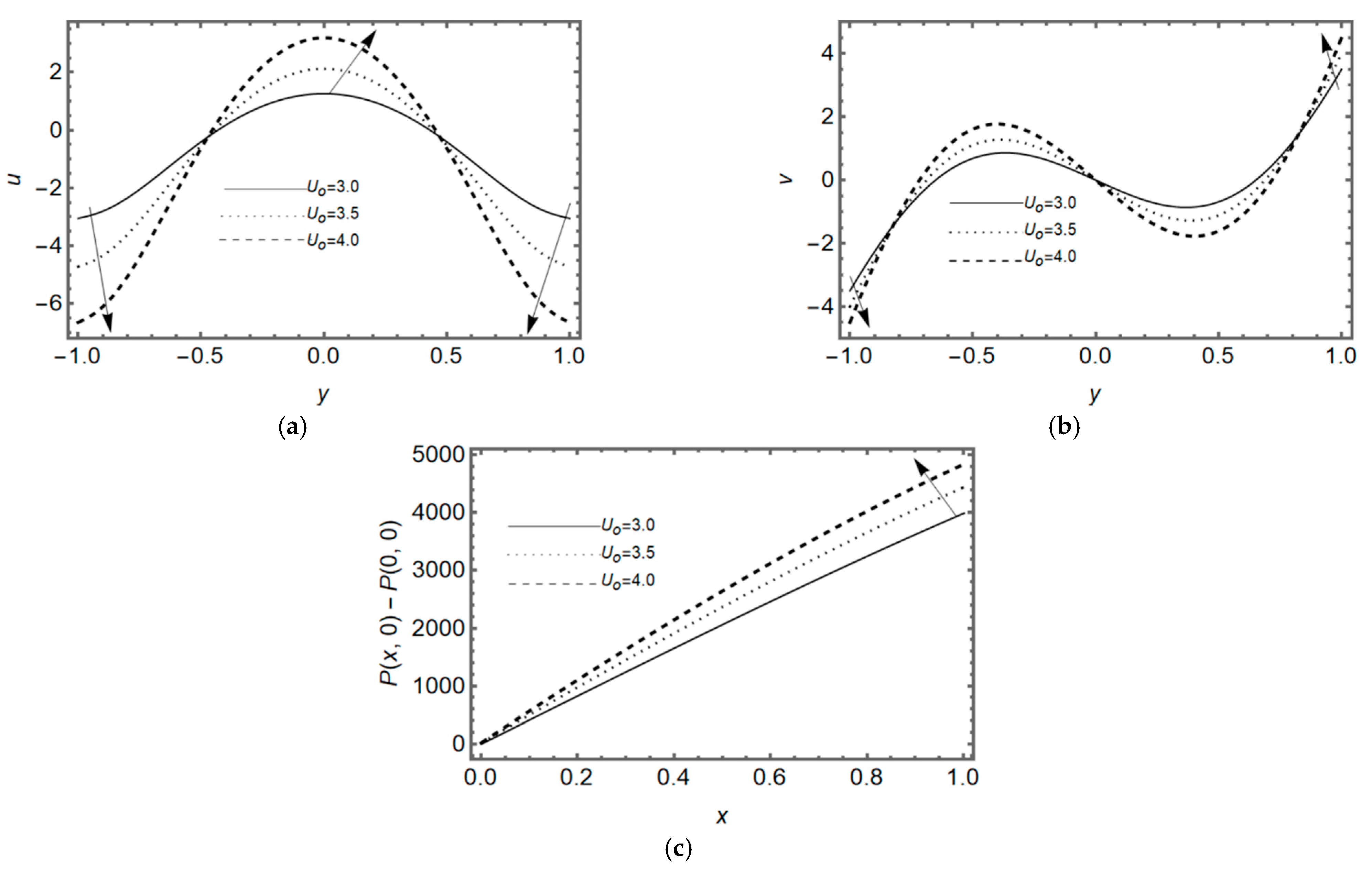
3.1. Effect of Reynold’s Number

Figure 2a,b display the impact of inertial forces at the middle region of the slit that appears due to Reynold’s number. This figure analyzes that axial flow is maximum at the center of the slit due to the presence of pressure gradient. The graphs also show that the flow in the vertical direction rises during activity (due to a non-zero Reynolds number). It also demonstrates the sharp rise in vertical velocity near the wall of the slit due to linear re-absorption in the synovium. Figure 2c shows that the pressure difference becomes more intense during activity (in the presence of Reynold’s number), and it also rises rapidly near the exit region. Essentially, it indicates that during the flow of synovial fluid in the synovial membrane, inertial forces take supremacy over viscous forces.

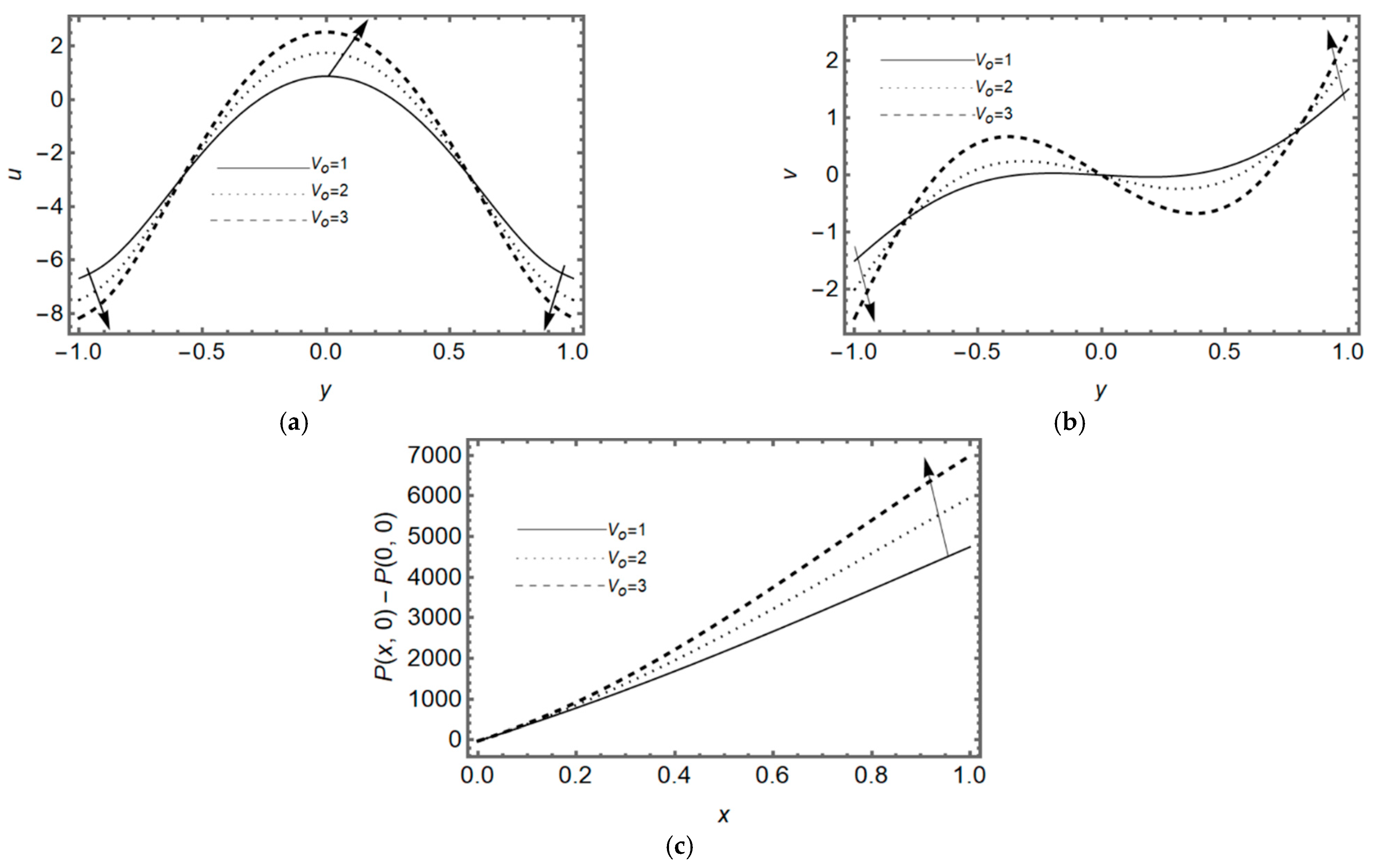
3.2. Effect of Re-Absorption Velocity V 0 x + U 0

Figure 3a,b shows the impact of the permeability of the membrane on the SF flow; this figure portrays the increasing effect of permeability on axial and transverse flow near the membrane. This graph indicates that the linear re-absorption causes an increase in axial and transverse flow due to the lubricated membrane, but the vertical flow rises in forward direction for the upper and lower regions. Figure 3c presents the effect of linear re-absorption V 0   on the pressure difference and displays the rising impact on the pressure distribution.
Figure 4a,b display the variation in axial and transverse velocity against the constant rate of re-absorption, which shows that the flow of synovial fluid along and transverse to the SM rises due to the appropriate viscosity of the synovial fluid. Figure 4c displays that the pressure difference between the two points in the synovial fluid flow rises when nutrients are re-absorbed at a constant rate in synovial fluid.

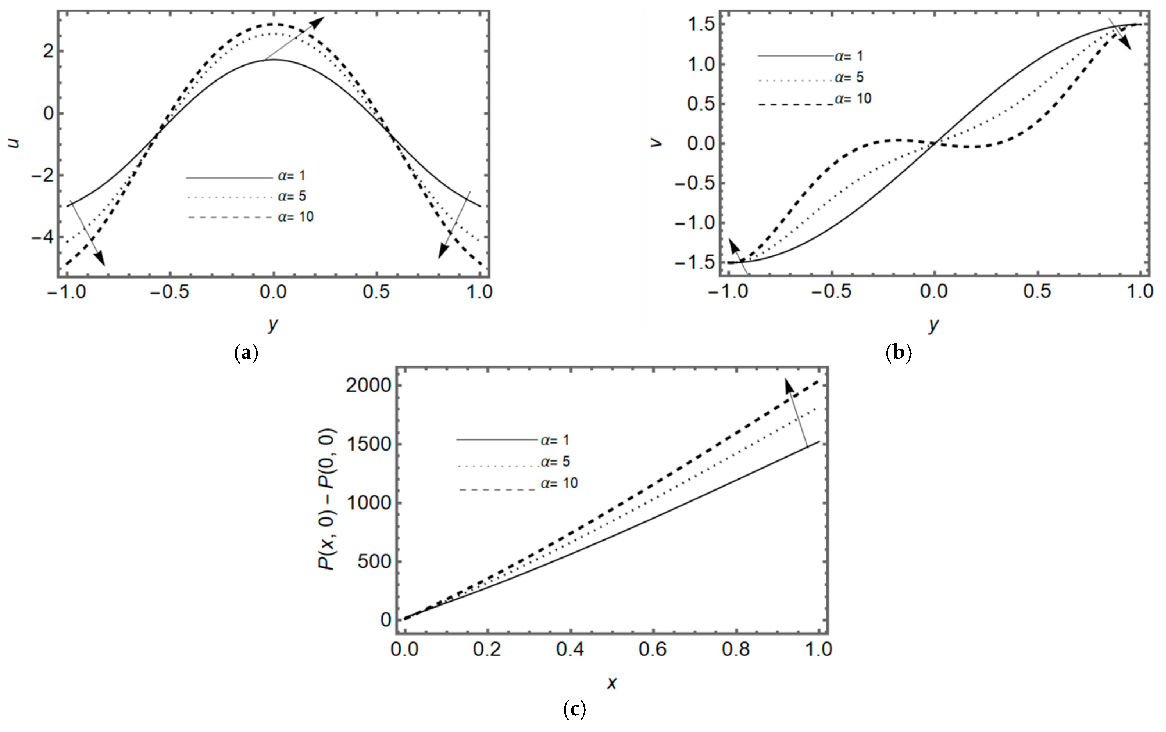
3.3. Effect of Couple-Stress Parameter α

Figure 5a,b display that the velocity in a horizontal direction rises for different couple-stress parameter (α) at the middle of the slit but the transverse velocity decay by the rising values of couple stress parameter. Furthermore, it is seen that axial velocity increases at the center of the slit and decreases near the walls due to lubricated permeable membrane. The pressure difference on the slit is shown in Figure 5c for various values of α which rises by the couple stress parameters; it shows the rotation of fluid particles and helps to flow the fluid also more pressure in synovial fluid is required in case of lubricated permeable slit.

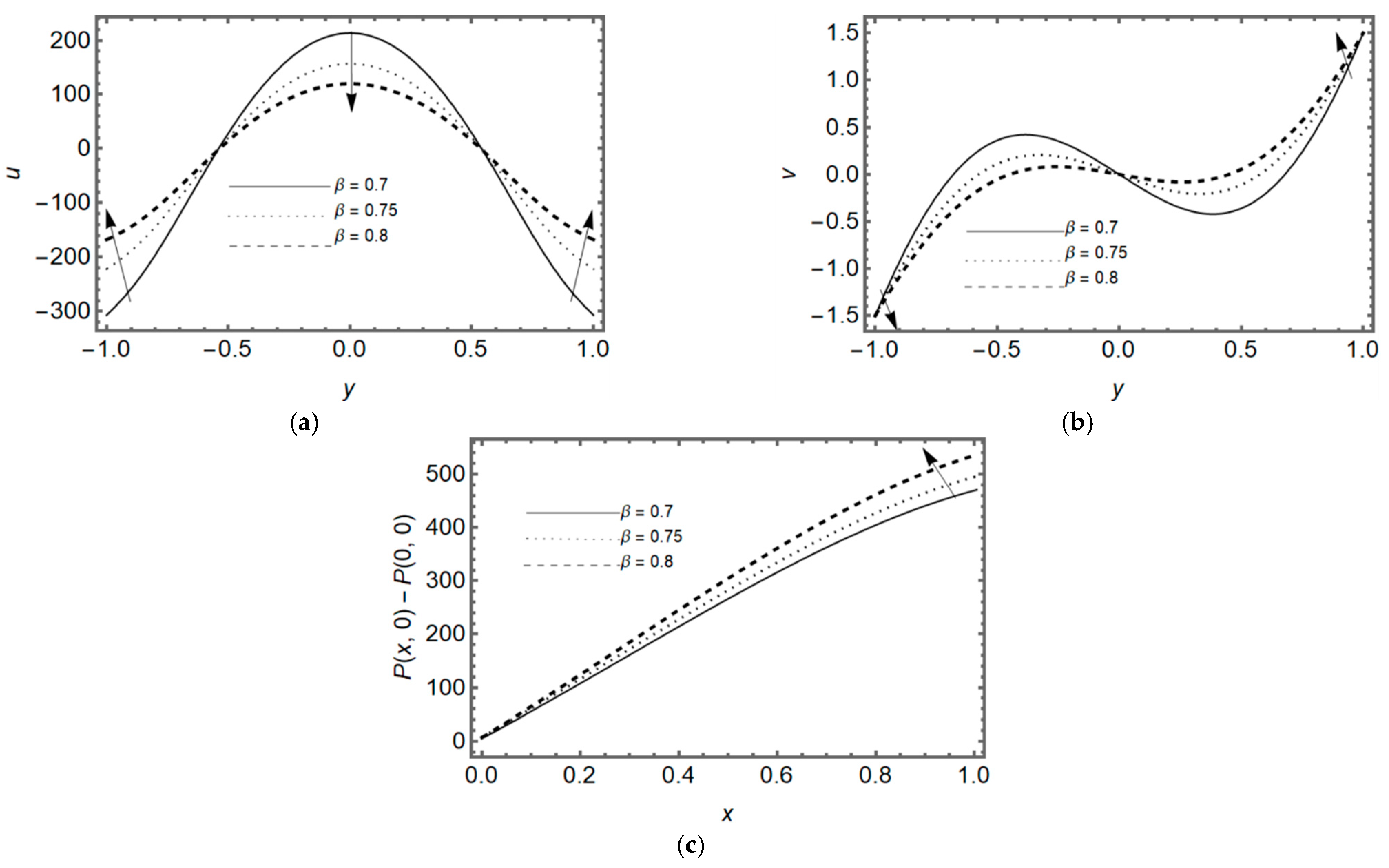
3.4. Effect of Slip Parameter β

Figure 6a,b display that the axial and transverse velocity decay for different slip parameters β at the middle of the slit. Furthermore, it is seen that axial velocity decays in the reverse direction near the walls due to the lubricated permeable membrane. The pressure difference on the slit is shown in Figure 6c for various values of slip parameter β , it shows that the lubrication on membrane helps to increase the pressure in synovial fluid near the exit region of the slit.

4. Concluding Remarks

The current study observes the impact of a lubricated membrane and linear re-absorption of nutrients in synovial fluid during movement or running. A two-dimensional couple stress fluid model through a permeable lubricated slit with linear re-absorption at the wall is assumed to observe the flow properties of synovial fluid. This model produces the complex non-linear partial differential equations that are solved by applying the Langlois approach with mixed boundary conditions. This study calculates the analytical findings of flow characteristics, including shear stress, pressure difference, and velocity profile for the smooth surface and non-porous medium. This study reveals that the presence of inertial forces supports the decelerating flow in axial and transverse directions but enhances the pressure difference.
In this study, we have ignored surface roughness and the effect of porous medium also the bending effects of synovial membrane that will be discussed in future work.

Author Contributions

Conceptualization, K.M. and A.M.S.; methodology, K.M.; software, A.A.; validation, K.M. and A.A.; formal analysis, A.M.S.; writing—original draft preparation, A.A.; writing—review and editing, A.B.M.; visualization, A.A.; supervision, K.M.; project administration, K.M. All authors have read and agreed to the published version of the manuscript.

Funding

This research received no external funding.

Data Availability Statement

No new data were created or analyzed in this study. Data sharing is not applicable to this article.

Conflicts of Interest

The authors declare no conflict of interest.

Appendix A

c 1 = c 3 = 0 ,         c 2 = 3 α 2 h α 2 h 2 β cosh h α 2 α β sinh h α 2 h α 3 + h α 2 h 3 β cosh h α + 6 1 + h α 2 β sinh h α
c 4 = α 3 c o s h [ h α ] 2 h α ( 3 + h 2 α 2 3 h α 2 β ) c o s h [ h α ] + 6 ( 1 + h α 2 β ) s i n h [ h α ] ,
c 5 = 3 2 h α 3 h α 2 h + 3 β c o s h h α 6 1 h α 2 β s i n h h α ,   c 6 = c 5 .
d 1 = d 3 = 0 ,         d 2 = 3 α h ( ( 2 + h α 2 ( h 2 β ) ) c o s h [ h α ] + 2 α β s i n h [ h α ] ) 4 W ( h α ( 3 + h α 2 ( h 3 β ) ) c o s h [ h α ] + 3 ( 1 + h α 2 β ) s i n h [ h α ] )
d 4 = α 3 h cosh h α 4 W h α 3 + h α 2 h 3 β cosh h α + 3 1 + h α 2 β sinh h α ,
d 5 = 3 h 4 W ( h α ( 3 + h α 2 ( h 3 β ) ) c o s h [ h α ] + 3 ( 1 + h α 2 β ) s i n h [ h α ] ) ,   d 6 = d 5 .
g x = 3   α 6 δ R e ( V 0 x + U 0 ) ( h W x ( 2 U 0 + V 0 x ) ) 4 W ( h α ( 3 + h α 2 ( h 3 β ) ) c o s h [ h α ] + 3 ( 1 + h α 2 β ) s i n h [ h α ] ) 2 ,
f y = y 3 α 2 + y 3 α 2 c o s h 2 h α + 6 β s i n h h α y α c o s h y α + s i n h y α + α c o s h h α y α 3 h 2 + y 2 + 6 h β c o s h y α + 3 h 2 y 2 2 h β s i n h y α

References

  1. Yin, W.; Frame, M.D. Biofluid Mechanics: An Introduction to Fluid Mechanics, Macrocirculation, and Microcirculation; Academic Press: Cambridge, MA, USA, 2011. [Google Scholar]
  2. Lai, W.M.; Kuei, S.C.; Mow, V.C. Rheological equations for synovial fluids. J. Biomech. Eng. 1978, 100, 169–186. [Google Scholar] [CrossRef]
  3. Ouerfelli, N.; Vrinceanu, N.; Mliki, E.; Amin, K.A.; Snoussi, L.; Coman, D.; Mrabet, D. Rheological behavior of the synovial fluid: A mathematical challenge. Front. Mater. 2024, 11, 1386694. [Google Scholar] [CrossRef]
  4. Singh, V.; Ganapathy, H.; Thanka, J. Synovial Fluid Analysis and Biopsy in Diagnosis of Joint Diseases. J. Pharm. Res. Int. 2021, 33, 1–11. [Google Scholar] [CrossRef]
  5. Hasnain, S.; Abbas, I.; Al-Atawi, N.O.; Saqib, M.; Afzaal, M.F.; Mashat, D.S. Knee synovial fluid flow and heat transfer, a power law model. Sci. Rep. 2023, 13, 18184. [Google Scholar] [CrossRef]
  6. Maqbool, K.; Siddiqui, A.M.; Mehboob, H.; Jamil, Q. Study of non-Newtonian synovial fluid flow by a recursive approach. Phys. Fluids 2022, 34, 111903. [Google Scholar] [CrossRef]
  7. Maqbool, K.; Siddiqui, A.M.; Mehboob, H.; Tahir, A. Dynamics of non-Newtonian synovial fluid through permeable membrane with periodic filtration. Int. J. Mod. Phys. B 2024, 38, 2450251. [Google Scholar] [CrossRef]
  8. Ramanaiah, G. Squeeze films between finite plates lubricated by fluids with couple stress. Wear 1979, 54, 315–320. [Google Scholar] [CrossRef]
  9. Ramanaiah, G.; Sarkar, P. Slider bearings lubricated by fluids with stress. Wear 1979, 52, 27–36. [Google Scholar] [CrossRef]
  10. Sinha, P.; Singh, C. Couple stresses in the lubrication of rolling contact bearings considering cavitation. Wear 1981, 7, 85–98. [Google Scholar] [CrossRef]
  11. Hayat, T.; Sajjad, R.; Alsaedi, A.; Muhammad, T.; Ellahi, R. On squeezed flow of couple stress nanofluid between two parallel plates. Results Phys. 2017, 7, 553–561. [Google Scholar] [CrossRef]
  12. Bashir, S.; Sajid, M. Flow of two immiscible uniformly rotating couple stress fluid layers. Phys. Fluids 2022, 34, 062101. [Google Scholar] [CrossRef]
  13. Madasu, K.P.; Sarkar, P. Couple stress fluid past a sphere embedded in a porous medium. Arch. Mech. Eng. 2022, 69, 5–19. [Google Scholar] [CrossRef]
  14. Ahmed, S.; Bég, O.A.; Ghosh, S.K. A couple stress fluid modeling on free convection oscillatory hydromagnetic flow in an inclined rotating channel. Ain Shams Eng. J. 2014, 5, 1249–1265. [Google Scholar] [CrossRef]
  15. Srivastava, L.M. Flow of couple stress fluid through stenotic blood vessels. J. Biomech. 1985, 18, 479–485. [Google Scholar] [CrossRef]
  16. Ozan, S.C.; Labrosse, G.; Uguz, A.K. A model of synovial fluid with a hyaluronic acid source: A numerical challenge. Fluids 2021, 6, 152. [Google Scholar] [CrossRef]
  17. Frisbie, D.D.; Al-Sobayil, F.; Billinghurst, R.C.; Kawcak, C.E.; McIlwraith, C.W. Changes in synovial fluid and serum biomarkers with exercise and early osteoarthritis in horses. Osteoarthr. Cartil. 2008, 16, 1196–1204. [Google Scholar] [CrossRef]
  18. Koh, A.S. Converging Biological Effects of Physical Activity on Cardiovascular Health in Ageing. Ph.D. Thesis, University of Dundee, Dundee, Scotland, UK, June 2024. [Google Scholar]
  19. Hahn, A.K.; Batushansky, A.; Rawle, R.A.; Lopes, E.P.; June, R.K.; Griffin, T.M. Effects of long-term exercise and a high-fat diet on synovial fluid metabolomics and joint structural phenotypes in mice: An integrated network analysis. Osteoarthr. Cartil. 2021, 29, 1549–1563. [Google Scholar] [CrossRef]
  20. Raja, U.A.; Siddique, J.I.; Ahmed, A. Biomechanical response of soft tissues during passage of synovial fluid in compression. Int. J. Comput. Methods Eng. Sci. Mech. 2023, 24, 182–192. [Google Scholar] [CrossRef]
  21. Haward, S.J. Synovial fluid response to extensional flow: Effects of dilution and intermolecular interactions. PLoS ONE 2014, 9, e92867. [Google Scholar] [CrossRef]
  22. Bridges, C.; Karra, S.; Rajagopal, K.R. On modeling the response of the synovial fluid: Unsteady flow of a shear-thinning, chemically-reacting fluid mixture. Comput. Math. Appl. 2010, 60, 2333–2349. [Google Scholar] [CrossRef]
  23. Oates, K.M.; Krause, W.E.; Jones, R.L.; Colby, R.H. Rheopexy of synovial fluid and protein aggregation. J. R. Soc. Interface 2006, 3, 167–174. [Google Scholar] [CrossRef] [PubMed]
  24. Mow, V.C. The role of lubrication in biomechanical joints. J. Lubr. Technol. 1969, 91, 320–326. [Google Scholar] [CrossRef]
  25. Hron, J.; Málek, J.; Pustějovská, P.; Rajagopal, K.R. On the modeling of the synovial fluid. Adv. Tribol. 2010, 1, 104957. [Google Scholar] [CrossRef]
  26. Ruggiero, A.; Gómez, E.; D’ Amato, R. Approximate closed-form solution of the synovial fluid film force in the human ankle joint with non-Newtonian Lubricant. Tribol. Int. 2013, 57, 156–161. [Google Scholar] [CrossRef]
  27. Pánek, P.; Kodým, R.; Šnita, D.; Bouzek, K. Spatially two-dimensional mathematical model of the flow hydrodynamics in a spacer-filled channel–the effect of inertial forces. J. Membr. Sci. 2015, 492, 588–599. [Google Scholar] [CrossRef]
  28. Siddiqui, A.M.; Haroon, T.; Shahzad, A. Hydrodynamics of viscous fluid through porous slit with linear absorption. Appl. Math. Mech. 2016, 37, 361–378. [Google Scholar] [CrossRef]
  29. Siddiqui, A.M.; Azim, Q.A.; Gawo, G.A.; Sohail, A. Analytical approach to explore theory of creeping flow with constant absorption. Sens. Int. 2024, 5, 100250. [Google Scholar] [CrossRef]
Figure 1. Geometry of synovial fluid flow through the synovial membrane in the knee joint.
Lubricants 13 00196 g001
Figure 2. (ac) Effect of Reynolds number on horizontal velocity, vertical velocity and pressure distribution.
Lubricants 13 00196 g002
Figure 3. (ac) Effect of re-absorption parameter   V 0   on horizontal velocity, vertical velocity and pressure distribution.
Lubricants 13 00196 g003
Figure 4. (ac) Effect of re-absorption parameter   U 0   on horizontal velocity, vertical velocity, and pressure.
Lubricants 13 00196 g004
Figure 5. (ac) Effect of the couple-stress parameter α on horizontal velocity, vertical velocity, and pressure distribution.
Lubricants 13 00196 g005
Figure 6. (ac) Effect of slip parameter β on horizontal velocity, vertical velocity, and pressure distribution.
Lubricants 13 00196 g006
Disclaimer/Publisher’s Note: The statements, opinions and data contained in all publications are solely those of the individual author(s) and contributor(s) and not of MDPI and/or the editor(s). MDPI and/or the editor(s) disclaim responsibility for any injury to people or property resulting from any ideas, methods, instructions or products referred to in the content.

