A Numerical Procedure Based on Orowan’s Theory for Predicting the Behavior of the Cold Rolling Mill Process in Full Film Lubrication


1
Department of Engineering University of Perugia Via G. Duranti 1, 06125 Perugia, Italy
2
Department of Information Engineering and Mathematics, University of Siena, Via Roma 56, 53100 Siena, Italy
3
Department of Advanced Robotics, Istituto Italiano di Tecnologia, 16163 Genoa, Italy
*
Author to whom correspondence should be addressed.
Lubricants 2020, 8(1), 2; https://doi.org/10.3390/lubricants8010002
Submission received: 23 October 2019
/
Revised: 9 December 2019
/
Accepted: 11 December 2019
/
Published: 18 December 2019
Abstract
:In this paper, a numerical model for predicting the working parameters of the cold rolling mill process in full film lubrication is presented. The model is useful from an industrial point of view, because it can forecast the thickness reduction of the metal sheet and the pressure trend, so that the rolling mill process parameters can be regulated to obtain a specific output thickness. Experimental tests were performed, and results are compared to the theoretical ones resulting from the model. The novelty of the proposed model is that it combines Orowan’s theory for the plastic deformation analysis with the Reynolds equation in full film lubrication and the continuity conditions. The lubricant flow and viscosity are studied, taking in account their dependence on pressure and temperature. The proposed model describing the full film regime is also compared to another one, previously proposed by the authors, based on the well-known slab analysis and sharing with it the representation of the lubrication regime, the mathematical procedure, and the boundary conditions. The results show that the proposed model provides a better prediction of the working parameters with respect to the model based on the slab analysis.

1. Introduction
Rolling mill is a metal forming process in which a metal strip passes between one or more stands of mated rolls, which induce a plastic deformation. The process can lead to a permanent reduction of thickness and to an elongation of the metal sheet, if the rolls are smooth, and to permanent modifications of the material section if the rolls are shaped. The rolling mill process can be performed in hot or cold conditions, and represents the first stage of production that brings the raw material to a semi-finished or finished product.
The plastic deformation occurring in the rolling mill process can be modelled and studied according to various methods proposed in the scientific literature.
Slab analysis is a widely diffused method for evaluating the contact pressure in cold rolling processes [1,2,3,4,5,6]; it is based on Von Karman’s theory and assumes a homogeneous plastic deformation in the strip thickness direction [7].
Finite element methods (FEMs) have also been used in model rolling processes, owing to their versatility and capability to manage complex boundary conditions [8,9,10]. The main advantage of FEM with respect to slab analysis is the possibility of removing basic assumptions on stress distributions. Furthermore, FEM can identify pressure distribution with more accuracy [11].
In the models presented in the works of [1,2,3,4,5,6,7,8,9,10,11], the influence of lubrication is not considered, but in the cold rolling mill process, a layer of lubricant is sprayed on the interface between the working rolls and the strip, to guarantee optimal superficial characteristics on high mechanical resistance metal strips. In fact, the use of lubricants reduces the friction and wear levels, ensures dimensional accuracy, and enhances the surface finish quality of the final product.
From the modelling and analysis point of view, however, the lubricant introduces significant issues, as a close interaction arises between metal strip deformation and lubricant fluid film flow; moreover, the lubricant influences the plastic deformation processes [12]. Film thickness is the most important parameter of a lubricated contact [13,14], even if experimental data are often deduced in dry conditions.
Rolling mill models considering the presence of lubricants are presented in some works in the scientific literature [15,16,17,18,19,20,21,22,23]. Lugt et al. [21] presented a model of the rolling mill process, also considering the metal strip elastic deformation in the inlet and outlet zone. Szeri and Wang developed an elasto-plasto-hydrodynamic numerical model for cold rolling mill processes, using slab analysis to manage strip deformation [22]. In the work of [23], a model of the cold rolling mill process was presented, considering the hypothesis of rigid strip and plastic deformation in the work zone, according to the slab analysis model. The present paper continues and extends previously obtained models on the rolling mill subject [23], and presents new results. In particular, a numerical model for predicting the working parameters of the cold rolling mill process in full film lubrication is developed and implemented, improving prior models and studying the cold rolling mill process in cylindrical coordinates.
The novelty of the proposed model over the models presented in the works of [1,2,3,4,5,6,7,8,9,10,11] is that the influence of lubricants is considered. The novelty with respect to the presented previous models [12,13,14,15,16,17,18,19,20,21,22,23] is that the new model combines Orowan’s inhomogeneous theory [24] for plastic deformation with the Reynolds equation in full film lubrication and the continuity conditions. The new proposed model presented in this paper and the previous model based on the slab analysis [23] share the representation of the lubrication regime, the mathematical procedure, and the boundary conditions, but in the new model, the plastic deformation of metal strips is described by means of Orowan’s inhomogeneous theory, instead of the slab analysis.
The lubricant flow and viscosity are studied, considering their dependence on pressure and temperature. The model can forecast the thickness reduction of the metal sheet and the pressure trend, so that the rolling mill process parameters can be regulated to obtain a specific output thickness. The experimental results are compared to the theoretical ones resulting from both the new and the previous model [23], in order to assess the prediction error.
The results demonstrated that the proposed model provides a better prediction of the working parameters and the thickness reduction rate with respect to the model based on the slab analysis.
2. Plastic Deformation Model
Typically, rolling processes are analyzed by dividing the modelling domain in three parts: (i) the inlet zone, where the film pressure increases from the external atmospheric value to an operating value allowing metal plastic deformation; (ii) the work zone, where the metal strip undergoes a plastic deformation, of which the final effect is a thickness reduction; (iii) the outlet zone, where the fluid film pressure decreases again, up to the atmospheric value. Each phase can be modelled with different constitutive equations.
For the evaluation of the pressure distribution in the work zone, an analytical model was introduced. The equations describing the deformation of the metal sheet implemented in this work are based on Orowan’s inhomogeneous theory [24], allowing a more accurate analysis of the interaction between work rolls and metal sheet with respect to the slab analysis, and the ability to describe more complex stress distributions. For instance, in the work of [25], it was applied to predict the deformation of a three-layered sheet. In this work, Orowan’s theory-based model was integrated with a full film lubrication model, in order to describe a cold rolling mill process.
- -
- ϕ (rad) is the rolling angle
- -
- θ is an angular variable varying between zero and ϕ
- -
- x is the horizontal coordinate on the rolling axis
- -
- y is the vertical coordinate perpendicular to the rolling axis
- -
- ϕ0 (rad) is the rolling angle corresponding to the beginning of the inlet zone
- -
- ϕiw (rad) is the rolling angle corresponding to the end of the inlet zone and the beginning of the work zone
- -
- ϕwo (rad) is the rolling angle corresponding to the end of the work zone and the beginning of the outlet zone
- -
- ϕ3 (rad) is the rolling angle corresponding to the end of the outlet zone
- -
- ω (rad/s) is the rolling speed
- -
- Si, So (m) are the strip thicknesses before and after the rolling mill process, Figure 1
- -
- R (mm) is the radius of the rolls
- -
- A, A′ (m2) are the inner and outer cylindrical sections used in the Orowan’s theory
- -
- F(ϕ) (N) is the horizontal force on the strip, Figure 2
- -
- p(ϕ) (Pa) is the pressure acting on the strip, Figure 2
- -
- (ϕ) (Pa) is the tangential stress on the strip planar surface, Figure 2
- -
- τ(ϕ) (Pa) is the tangential stress acting on the strip cylindrical section, Figure 2
- -
- t (ϕ) (Pa) is the radial pressure on the strip cylindrical section, Figures 2 and 3
- -
- Fτ (ϕ) and Ft (ϕ) (N) are the two components of the horizontal force F in the tangential and radial directions, respectively, Figures 2 and 3
- -
- is the , Figure 4
- -
- σs (MPa) is the material yield stress
- -
- y1(ϕ) (m) is the function expressing the profile of the strip measured from the longitudinal axis and its semi-thickness, Figures 2 and 5
- -
- y2 (ϕ) (m) is the function expressing the profile of the fluid film measured from the longitudinal axis and the semi-thickness of the strip and the fluid film together, Figure 5
- -
- h0(ϕ) (m) is the function expressing the semi-thickness of the fluid film at the beginning of the inlet zone, Figure 5
- -
- h(ϕ) (m) is the function expressing the semi-thickness of the fluid film
- -
- (m/s) is the velocity field with the horizontal component u and the vertical component v
- -
- u1(ϕ) (m/s) is the horizontal velocity at y1 (ϕ)
- -
- u2(ϕ) (m/s) is the horizontal velocity at y2 (ϕ)
- -
- u10 (m/s) is the horizontal velocity at y1 (ϕ0)
- -
- u13 (m/s) is the horizontal velocity at y1 (ϕ3)
- -
- v1(ϕ) (m/s) is the vertical velocity at y1 (ϕ)
- -
- v2(ϕ) (m/s) is the vertical velocity at y2 (ϕ)
- -
- μ (Pa∙s) is the lubricant viscosity
- -
- μ0 (Pa∙s) is the lubricant viscosity in standard conditions
- -
- γ (Pa−1), α (°C−1) are the two Barus constants
- -
- T (°C) is the temperature
- -
- f is the friction coefficient
- -
- a is Orowan’s parameter
- -
- Q (m3/s) is the lubricant flow rate
Subscript 1 refers to variables and constants regarding the surface of the metal sheet; subscript 2 refers to variables and constants regarding the surface of the fluid film in contact with the rolls.
A scheme of the system in dry conditions, and the main geometrical parameters, are represented in Figure 1. In the inhomogeneous theory, the rolled strip is divided into a series of elements: the generic element is defined by means of two cylindrical surfaces, indicated with A and A′ in Figure 1, and the roll’s surfaces, which are considered as planes. A sketch of a generic element and the forces acting on it is shown in Figure 2.
By considering the force equilibrium equation in the horizontal direction, the following equation can be obtained:
where R is the radius of the rolls, is the horizontal force, is the pressure, and is the tangential stress acting on the strip surface.
When modelling this process, the assumption commonly made is that the deformation is a locally homogeneous compression. In this paper, the deformation is considered inhomogeneous, so, to express as a function of , the tension state must be known.
The results derived by Prandtl and Naday [24], from the Hencky dissertation of the two-dimensional plastic deformation, allow to express the two tension components (t and τ) in the case of compression between two planar and not parallel surfaces (Figure 2) in angular coordinates as follows:
where t is the radial pressure and τ the tangential stress on the strip cylindrical section (as sketched in Figure 3), σs is the material yield stress, and θ is an angular variable varying between zero and ϕ.
The two components and of the horizontal force F are obtained by integration of the radial pressure and the tangential stress:
where w is defined as follows:
and y1(ϕ) is the function expressing the profile of the strip measured from the longitudinal axis and its semi-thickness (Figure 2 and Figure 5).
In the lubricated cold rolling mill process and in full film regime, the friction is very small and the component evaluated in Equation (4) can be neglected.
The mathematical relationship between F and p becomes the following:
Equation (7) and Equation (1) are combined so that the following expression describing the strip deformation is obtained:
Considerations about w
In Orowan’s theory, Equation (6) is expressed by:
where and f is the friction coefficient. Thus, when slip occurs between the mating surfaces, while when , the surfaces adhere. In the case of dry cold rolling mill processes, the function w takes into account the influence of the zone where the metal strip adheres to the rolls and of the zone where the strip slips. In presence of a lubricant, the contact takes place between the strip and the lubricant and between the lubricant and the rolls. In the case of this paper, the flow is laminar, a = 1, and w = 0.78, as shown in Figure 4. Thus, the mathematical relationship between the force F and the pressure p is influenced by this value of w, according to Equation (7).
The function was evaluated for different values of , as shown in Figure 4.
When ϕ varies between 0 and 30°, the average variation of w is lower than 0.2%, while the maximum variation, occurring for , is equal to 0.3% (red curves in Figure 4). For this reason, the derivative in Equation (8) can be neglected.
In particular, the function can be approximated by the polynomial expression (blue dashed curve in Figure 4):
3. Global Model
When the lubricant is sprayed between the working rolls, a full film lubrication regime is established. In this work, the following assumptions were considered in the global model of the process:
- -
- the material is rigid and perfectly plastic;
- -
- strain-hardening effects are negligible;
- -
- surfaces are considered perfectly smooth (the roughness of contact surfaces being neglected);
- -
- strip width is much larger than strip thickness, thus the problem can be considered in two dimensions;
- -
- lubricant is uncompressible;
- -
- lubricant flow is laminar;
- -
- lubricating area is much smaller than the roll circumference;
- -
- lubricant film thickness is much smaller than material thickness reduction;
- -
- inertia forces are negligible;
- -
- rolls are rigid.
The last hypothesis can be accepted in presence of lubrication, as errors in the evaluation of the contact curve are negligible, as the mean pressure on the rolls decreases. On the contrary, in dry conditions, the assumption of rigid rolls would lead to a wrong evaluation of the contact curve [24,26].
3.1. Viscosity
The viscosity of the lubricant was assumed to vary according to the Barus law, depending on the temperature T and on the pressure p:
where γ and α are the two Barus constants. In this work, the considered lubricant was an oil/water emulsion and the Barus constants were γ = 10−8 Pa−1 and α = 0.0163989 °C−1.
In the studied rolling mill plant, the oil outlet temperature was 40 °C and the dependence on pressure and temperature was also analyzed.
3.2. Model Equations and Domains
The global model of the cold rolling mill process was developed considering the lubrication regime, described by the Reynolds equation, the continuity condition, and the plastic deformation model, based on Orowan’s theory. Three different domains over the surface of the metal sheet under production were considered and treated with different equations: the inlet, the work, and the outlet zone domains, as shown in Figure 5.
In the inlet zone, the pressure within the lubricant film between the rolls and the rigid strip rises rapidly until the deformation of the strip starts at the inlet edge of the work-zone. In this domain, the shape of the fluid film is known. If ϕ0 represents the angle at the beginning of the inlet zone, y1(ϕ) is the function expressing the profile of the strip measured from the longitudinal axis and its semi-thickness, and y2(ϕ) is the function expressing the profile of the fluid film measured from the longitudinal axis and the semi-thickness of the strip and the fluid film together; and are given by the following:
where h0 is the function expressing the semi-thickness of the fluid film at the beginning of the inlet zone and Si is the metal sheet thickness (Figure 5).
Defining the velocity field as , the components are as follows:
where ω is the angular speed of the rolls, supposed as constant, and is the initial horizontal velocity at y1(ϕ0).
In the inlet zone, the Reynolds equation assumes the following expression, where the squeeze effect is also considered:
where .
The integration was performed by a feed-forward numerical procedure with as the boundary condition. This procedure stops when the yield stress is reached: . In correspondence of this situation, the end of the inlet zone is evaluated: .
In the work zone, the three governing equations are the Reynolds, the continuity, and Orowan’s equations:
The variables are , , and , and the feed-forward integration procedure stops when . In correspondence of this situation, the end of the work zone is evaluated .
In the outlet zone, the shape of the fluid film is known, and the thickness of the strip at the beginning section and the thickness of the fluid film from the beginning of the outlet zone are as follows:
The corresponding components of the velocity are as follows:
where is the final horizontal velocity at y1(ϕwo) and y1(ϕ3).
The Reynolds equation assumes the following expression:
The feed-forward integration procedure stops when . In correspondence of this situation, the end of the outlet zone is evaluated .
4. Results and Discussion
The following input data were used for the numerical evaluation of the model previously introduced:
- -
- R = 0.255 m
- -
- ω = 60.13 rad/s
- -
- μ0 = 5 Pa∙s
- -
- Si = 12 × 10−4 m
- -
- u10 = 11.7 m/s
- -
- σs = 730 MPa
- -
- Q = 2.74 × 10⁻⁴ m3/s
- -
- γ = 10−8 Pa−1
where Q is the lubricant flow rate. Such data were taken from a real rolling mill process.
Figure 6 shows the dimensionless relative pressure p* of the lubrication film in function of the relative angle ϕ* for both of the models: the first one is based on Orowan’s theory and presented in this paper, and the second one is based on the slab analysis presented in the work of [23]. p* is the ratio between the pressure and the plastic yield stress, while ϕ* is the ratio between the actual value of ϕ and ϕiw. ϕiw represents the value of the angle at the end of the inlet zone and beginning of the work zone.
From this picture, one can observe that the trend of the pressure in the inlet zone is superimposable for the two different models, but in the work and outlet zones, the pressure diagrams differ. In particular, the model based on Orowan’s theory predicts a higher value of the relative pressure, and also a bigger range of ϕ where the plastic deformation phase takes place, so that the Orowan’s work zone is wider.
The simulation parameters adopted here were relative to a real rolling plant used for experimental tests. Thus, the value of the metal sheet thickness (So) coming out from the rolling mill plant could be measured. All the tests were performed using the same working parameters and the same materials. In particular, the material used for the tests was a martensitic aging steel used for aeronautic and automotive applications, with a yield stress of 730 MPa and initial metal sheet thickness of 12 × 10−4 m. The rolling mill plant had rolls with a radius of 0.255 m and the basic working parameters used for the tests were as follows: a roll angular velocity of 60.13 rad/s, an initial horizontal velocity of the metal sheet of 11.7 m/s and an environmental temperature of 20 °C. The oil/water emulsion used as a lubricant had a value of μ0 equal to 5 Pa∙s, a flow rate of 2.74 × 10⁻⁴ m3/s, and an outlet temperature of 40 °C.
The measured value of So considered in this work is the mean value resulting after 10 tests in the same environmental conditions, as already mentioned. Table 1 shows the results of the experimental tests. Therefore, the mean value of So was compared with the ones predicted by the model proposed in this work and the one based on the slab analysis, as Table 2 summarizes.
The real strip thickness in the plant varies from Si = 1.240 mm to So = 0.898 mm. The model using Orowan’s theory predicts So = 0.882 mm, while the model based on the slab analysis predicts So = 0.934 mm. This means that the real thickness reduction is equal to 27.6% and the thickness reduction predicted by Orowan’s theory and slab analysis are equal to 28.9% and 24.7%, respectively.
Thus, the percentage error in the thickness reduction predicted by the models involving Orowan’s theory and the slab analysis are −1.3% and +2.9%, respectively.
The model based on Orowan’s plastic deformation theory is more accurate in predicting the sheet thickness reduction, not only for the minor error percentage, but also because it overestimates the reduction, and this is in good agreement with the fact that the spring back of the metal sheet is not considered here.
Then, the model based on Orowan’s inhomogeneous theory was applied, also considering the influence of different viscosity models. In particular, it was applied considering a constant viscosity and a viscosity varying according to the Barus law as a function of pressure; Equation (11).
The results of the application of the model with different viscosities are reported in Figure 7. One can observe that, using the Barus law, the pressure in the work zone is higher, but the deformation zone is narrower.
Similarly, the influence of the temperature was also analyzed. Two temperature levels were considered: 40 °C, corresponding to the output temperature from the real rolling mill process at the real test plant, and 140 °C as a test temperature. In the proposed model, the temperature value affects the calculation of the viscosity, according to Equation (11).
Figure 8 shows the results in terms of film shape, applying Orowan’s theory and according to the Barus law. In Table 3, the numerical results are reported. From Figure 8 and from these results, one can observe that the extent of the work zone and the thickness reduction change with temperature: the work zone is wider, and the output thickness is smaller with lower temperatures.
5. Conclusions
This section is not mandatory, but may be added if there are patents resulting from the work reported in this manuscript.
In this paper, a model of the cold rolling mill process is proposed as an alternative to previously developed models. This paper aimed at properly defining the relationship between the lubricant flow rate and the reduction of thickness of the metal sheet, given the other operation parameters.
In the approach proposed in this work, the study of the plastic deformation is accomplished by using Orowan’s inhomogeneous theory, instead of the common slab analysis, and the influence of pressure and temperature on the viscosity is taken into account. The parameters involved in the process are the lubricant flow rate, the distance between the rolls, and the tension applied to the strip.
A real rolling mill plant was used as a test plant to gather experimental data for evaluating the model’s prediction error. All the tests were performed using the same working parameters and the same materials. From the application of the two models with the same working parameter of the real rolling mill plant, and comparing the results with experimental data, it results that the new approach entails a reduction of the percentage error in the prediction of the final thickness of the metal sheet and of the process parameters. The practical industrial perspective of the presented work is that the new model can be advantageously employed to predict the thickness reduction of metal sheets when a set of parameters is known. In this way, the cold rolling mill process can be regulated to obtain a fixed reduction of thickness.
Author Contributions
Conceptualization, M.C.V. and M.M.; Data curation, M.C.V., M.M., and S.L.; Formal analysis, M.C.V., M.M., and S.L.; Investigation, M.C.V., M.M., and S.L.; Methodology, M.C.V., M.M., and S.L.; Project administration, M.C.V.; Software, M.C.V. and M.M.; Supervision, M.C.V. and M.M.; Validation, M.C.V. and S.L.; Writing—original draft, M.C.V. and S.L.; Writing—review & editing, M.C.V. and S.L. All authors have read and agreed to the published version of the manuscript.
Funding
This research received no external funding.
Conflicts of Interest
The authors declare no conflict of interest.
References
- Ford, H. The theory of rolling. Metall. Rev. 1957, 2, 1–28. [Google Scholar] [CrossRef]
- Alexander, J.M. On the theory of rolling. Proc. R. Soc. Lond. A Math. Phys. Sci. 1972, 326, 535–563. [Google Scholar] [CrossRef]
- Valigi, M.C.; Papini, S. Analysis of chattering phenomenon in industrial S6-high rolling mill. Diagnostyka 2013, 14, 3–8. Available online: http://www.diagnostyka.net.pl/Issue-3-2013,3228 (accessed on 23 October 2019).
- Papini, S.; Valigi, M.C. Analysis of chattering phenomenon in industrial S6-high rolling mill. Part II: Experimental study. Diagnostyka 2016, 17, 27–32. Available online: http://www.diagnostyka.net.pl/Analysis-of-chattering-phenomenon-in-industrial-S6-High-rolling-mill-Part-II-experimental,65818,0,2.html (accessed on 23 October 2019).
- Valigi, M.C.; Rinchi, M. Chattering in rolling of advanced high strength steels. In Rolling of Advanced High Strength Steels: Theory, Simulation and Practice; CRC Presss: Boca Raton, FL, USA, 2017; pp. 522–565. [Google Scholar] [CrossRef]
- Valigi, M.C.; Cervo, S.; Petrucci, A. Chatter marks and vibration analysis in a S6-high cold rolling mill. Lect. Notes Mech. Eng. 2014, 5, 567–575. [Google Scholar] [CrossRef]
- Von Karman, T. On the theory of rolling. Z. Angew. Math. Mech. 1925, 5, 139–141. [Google Scholar]
- Lim, H.B.; Yang, H.I.; Kim, C.W. Analysis of the roll hunting force due to hardness in a hot rolling process. J. Mech. Sci. Technol. 2019, 33, 3783–3793. [Google Scholar] [CrossRef]
- Kamal, F.; Rath, S.; Acherjee, B. Process modelling of flat rolling of steel. Adv. Mater. Process. Technol. 2019, 5, 104–113. [Google Scholar] [CrossRef]
- Liu, C.; Hartley, P.; Sturgess, C.E.; Rowe, G.W. Elastic-plastic finite-element modelling of cold rolling of strip. Int. J. Mech. Sci. 1985, 27, 531–541. [Google Scholar] [CrossRef]
- Hwu, Y.; Lenard, J.G. A Finite Element Study of Flat Rolling. ASME J. Eng. Mater. Technol. 1988, 110, 22–27. [Google Scholar] [CrossRef]
- Moshkovich, A.; Perfilyev, V.; Rapoport, L. Effect of Plastic Deformation and Damage Development during Friction of fcc Metals in the Conditions of Boundary Lubrication. Lubricants 2019, 7, 45. [Google Scholar] [CrossRef] [Green Version]
- Jamali, H.U.; Al-Hamood, A.; Abdullah, O.I.; Senatore, A.; Schlattmann, J. Lubrication Analyses of Cam and Flat-Faced Follower. Lubricants 2019, 7, 31. [Google Scholar] [CrossRef] [Green Version]
- Ciulli, E.; Pugliese, G.; Francesco, F. Film Thickness and Shape Evaluation in a Cam-Follower Line Contact with Digital Image Processing. Lubricants 2019, 7, 29. [Google Scholar] [CrossRef] [Green Version]
- Wei, L.; Qu, Z.; Zhang, X.; Guo, Y.; Wang, K. Influence of rolling lubrication for self-excited vibration on tandem cold rolling mill. Adv. Mater. Res. 2013, 634–638, 2849–2854. [Google Scholar] [CrossRef]
- Liu, L.; Zang, Y.; Gao, Z. The influence of surface waviness on hydrodynamic lubrication behavior in cold rolling process. In Proceedings of the 2010 International Conference on Mechanic Automation and Control Engineering, MACE2010, Wuhan, China, 26–28 June 2010; Volume 5536705, pp. 3844–3847. [Google Scholar] [CrossRef]
- Liu, L.; Zang, Y.; Chen, Y. Study on the hydrodynamic lubrication behavior in cold rolling process. Adv. Mater. Res. 2011, 154–155, 731–737. [Google Scholar] [CrossRef]
- Chen, S.-Z.; Zhang, D.-H.; Sun, J.; Wang, J.-S.; Song, J. Online calculation model of rolling force for cold rolling mill based on numerical integration. In Proceedings of the 2012 24th Chinese Control and Decision Conference, CCDC 2012, Taiyuan, China, 23–25 May 2012; Volume 6244629, pp. 3951–3955. [Google Scholar] [CrossRef]
- Wu, C.; Zhang, L.; Qu, P.; Li, S.; Jiang, Z. A multi-field analysis of hydrodynamic lubrication in high speed rolling of metal strips. Int. J. Mech. Sci. 2018, 142–143, 468–479. [Google Scholar] [CrossRef]
- Lo, S.-W.; Yang, T.-C.; Lin, H.-S. The lubricity of oil-in-water emulsion in cold strip rolling process under mixed lubrication. Tribol. Int. 2013, 66, 125–133. [Google Scholar] [CrossRef]
- Lugt, P.M.; Wemekamp, A.W.; ten Napel, W.E.; van Liempt, P.; Otten, J.B. Lubrication in cold rolling: Elasto-plasto-hydrodynamic lubrication of smooth surfaces. Wear 1993, 166, 203–214. [Google Scholar] [CrossRef] [Green Version]
- Szeri, A.Z.; Wang, S.H. An elasto-plasto-hydrodynamic model of strip rolling with oil/water emulsion lubricant. Tribol. Int. 2004, 37, 169–176. [Google Scholar] [CrossRef]
- Valigi, M.C.; Malvezzi, M. Cold rolling mill process: A numerical procedure for industrial applications. Meccanica 2008, 43, 1–9. [Google Scholar] [CrossRef]
- Orowan, E. The calculation of roll pressure in hot and cold flat rolling. Proc. Inst. Mech. Eng. 1943, 150, 140–167. [Google Scholar] [CrossRef]
- Alexandrov, S.; Lyamina, E. Extension of Orowan’s method to analysis of rolling of three-layer sheets. Procedia Eng. 2017, 207, 1391–1396. [Google Scholar] [CrossRef]
- Roberts, W.L. Flat Processing of Steel; M. Dekker: New York, NY, USA, 1988; ISBN1 0824777808. ISBN2 9780824777807. [Google Scholar]
Figure 1.
The rolled strip in the inhomogeneous theory, main definitions.

Figure 2.
Single element of material and acting forces.

Figure 3.
Tension state (radial pressure t and tangential stress ) in a generic point of the element section.
Figure 3.
Tension state (radial pressure t and tangential stress ) in a generic point of the element section.
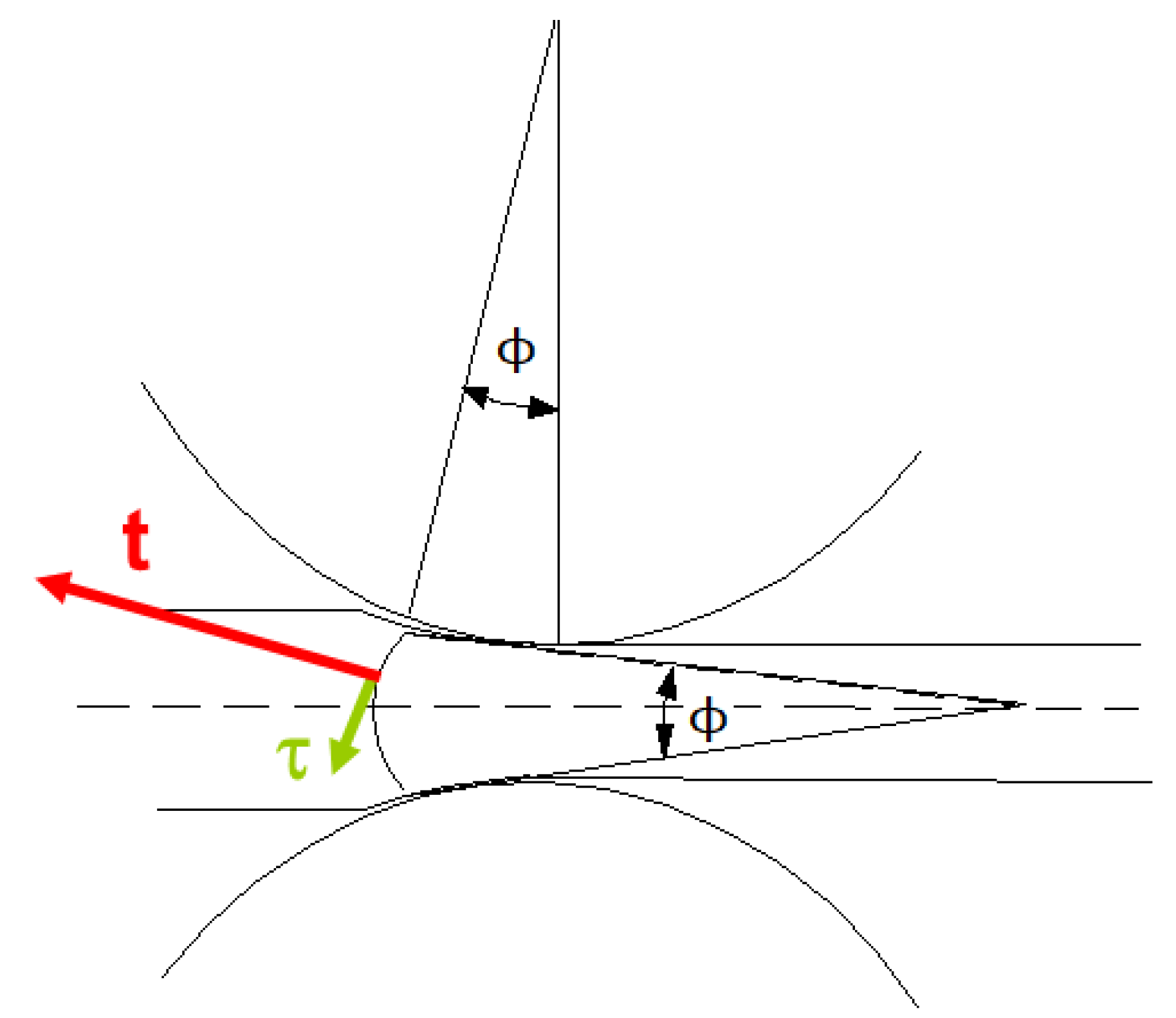
Figure 4.
Function . Red curves are obtained by varying ϕ between 0° and 30°; the blue curve represents the polynomial approximation evaluated by Equation (10).
Figure 4.
Function . Red curves are obtained by varying ϕ between 0° and 30°; the blue curve represents the polynomial approximation evaluated by Equation (10).

Figure 5.
Global model.
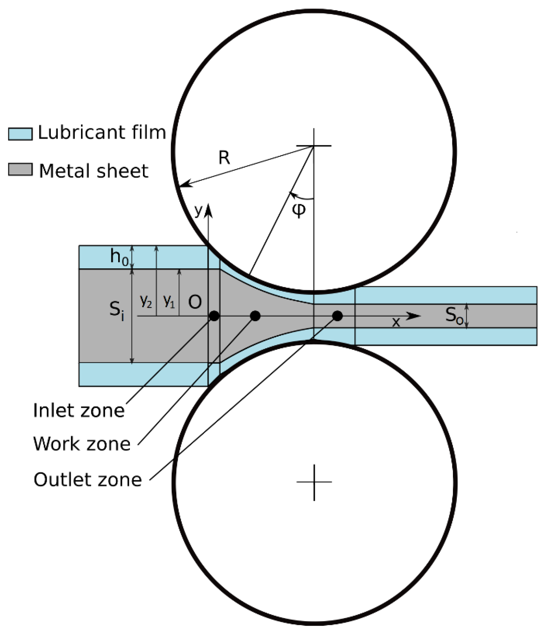
Figure 6.
Diagram p*-ϕ*: comparison of results obtained by Orowan’s theory (black curve) and the slab analysis (red curve).
Figure 6.
Diagram p*-ϕ*: comparison of results obtained by Orowan’s theory (black curve) and the slab analysis (red curve).

Figure 7.
Diagram p*-ϕ*: comparison of results obtained by Orowan’s theory with different models of viscosity.
Figure 7.
Diagram p*-ϕ*: comparison of results obtained by Orowan’s theory with different models of viscosity.

Figure 8.
Film shapes obtained by Orowan’s theory with different temperatures, where y1(ϕ*) and y2(ϕ*) are the profiles of the strip and of the fluid film from the longitudinal axis, respectively.
Figure 8.
Film shapes obtained by Orowan’s theory with different temperatures, where y1(ϕ*) and y2(ϕ*) are the profiles of the strip and of the fluid film from the longitudinal axis, respectively.


Table 1.
Experimental results.
| Test Number | Measured Value of So (Plant) |
|---|---|
| 1 | 0.898 mm |
| 2 | 0.899 mm |
| 3 | 0.898 mm |
| 4 | 0.899 mm |
| 5 | 0.898 mm |
| 6 | 0.899 mm |
| 7 | 0.897 mm |
| 8 | 0.899 mm |
| 9 | 0.897 mm |
| 10 | 0.896 mm |
Table 2.
Summary of results and comparison between the final thickness of the sheet: measured, evaluated with Orowan’s theory, and the slab analysis models.
Table 2.
Summary of results and comparison between the final thickness of the sheet: measured, evaluated with Orowan’s theory, and the slab analysis models.
| Variable | Measured Mean Value (Plant) | Orowan’s Model | Slab Analysis |
|---|---|---|---|
| So | 0.898 mm | 0.882 mm | 0.934 mm |
Table 3.
Summary of results and comparison between the final thickness: measured and evaluated with Orowan’s theory for different temperatures.
Table 3.
Summary of results and comparison between the final thickness: measured and evaluated with Orowan’s theory for different temperatures.
| Variable | Measured Mean Value (Plant) | T = 40 °C | T = 140 °C |
|---|---|---|---|
| So | 0.898 mm | 0.882 mm | 0.889 mm |
© 2019 by the authors. Licensee MDPI, Basel, Switzerland. This article is an open access article distributed under the terms and conditions of the Creative Commons Attribution (CC BY) license (http://creativecommons.org/licenses/by/4.0/).
Share and Cite
MDPI and ACS Style
Valigi, M.C.; Malvezzi, M.; Logozzo, S. A Numerical Procedure Based on Orowan’s Theory for Predicting the Behavior of the Cold Rolling Mill Process in Full Film Lubrication. Lubricants 2020, 8, 2. https://doi.org/10.3390/lubricants8010002
AMA Style
Valigi MC, Malvezzi M, Logozzo S. A Numerical Procedure Based on Orowan’s Theory for Predicting the Behavior of the Cold Rolling Mill Process in Full Film Lubrication. Lubricants. 2020; 8(1):2. https://doi.org/10.3390/lubricants8010002
Chicago/Turabian StyleValigi, Maria Cristina, Monica Malvezzi, and Silvia Logozzo. 2020. "A Numerical Procedure Based on Orowan’s Theory for Predicting the Behavior of the Cold Rolling Mill Process in Full Film Lubrication" Lubricants 8, no. 1: 2. https://doi.org/10.3390/lubricants8010002
Note that from the first issue of 2016, this journal uses article numbers instead of page numbers. See further details here.