Viscoelastic Effects during Tangential Contact Analyzed by a Novel Finite Element Approach with Embedded Interface Profiles


Abstract
1. Introduction
2. Materials and Methods
2.1. Proposed Solution Scheme for the Contact Problem
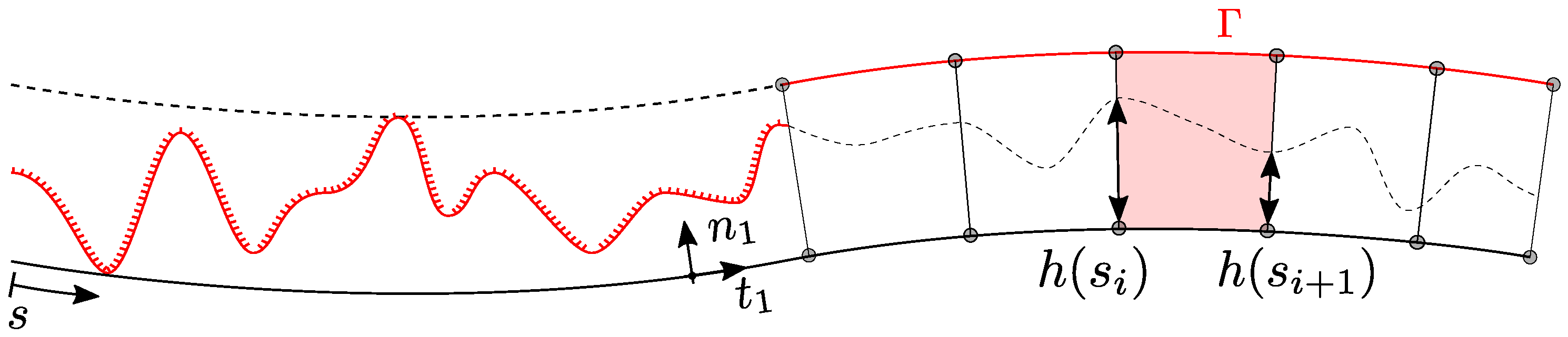
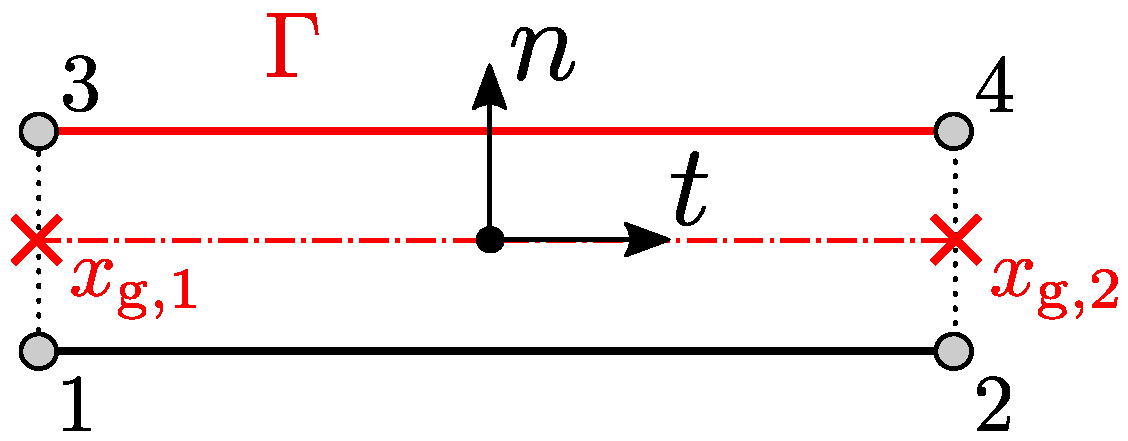
2.2. MPJR Formulation
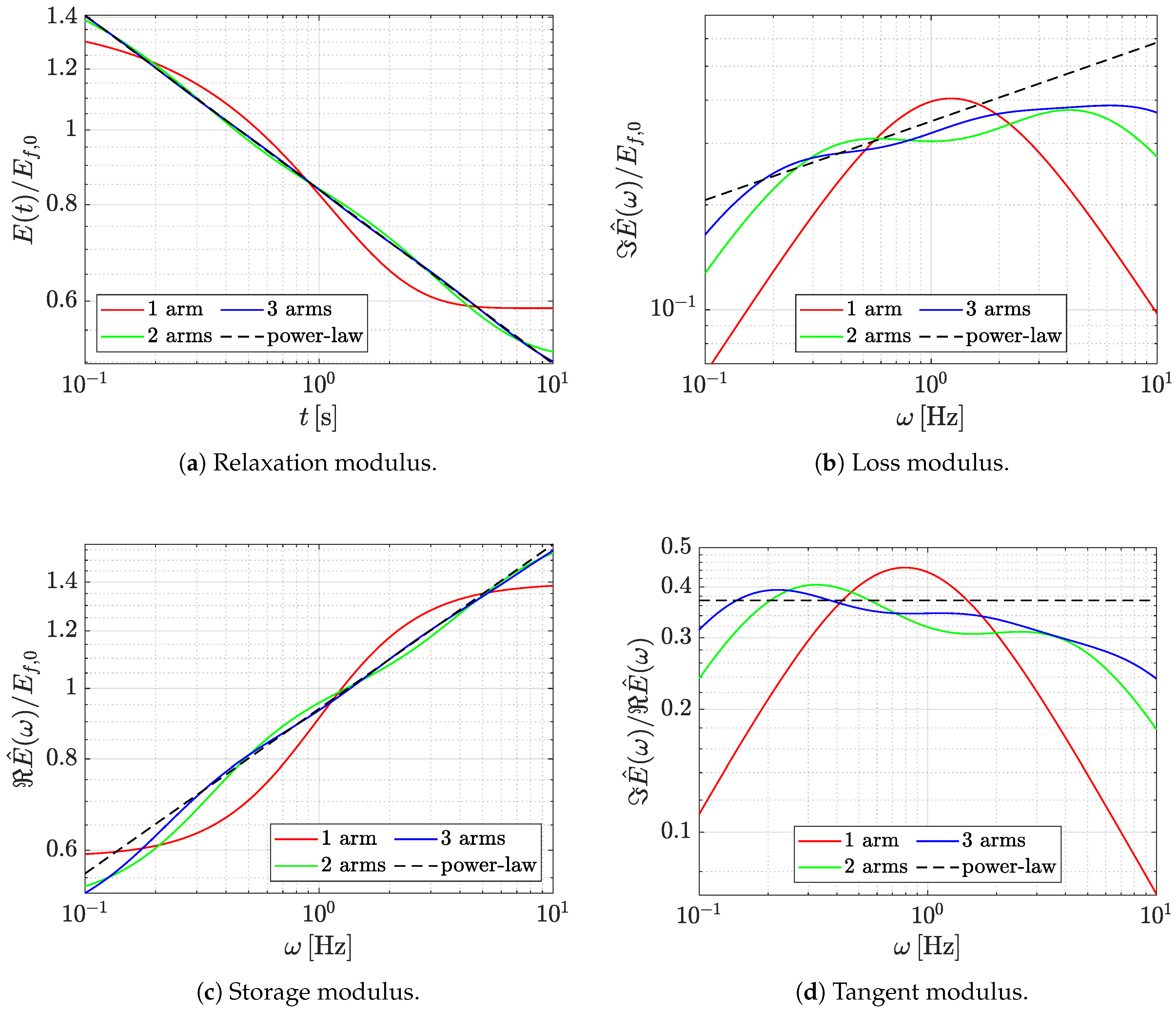
2.3. Rheological Model
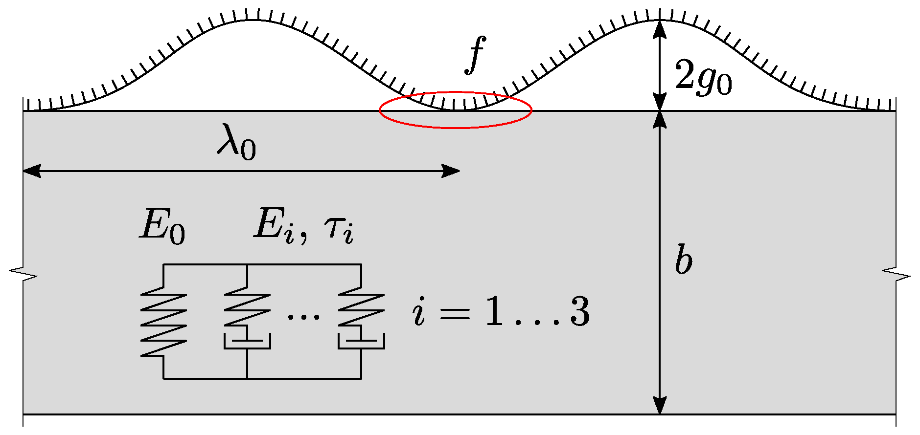
2.4. Problem Set Up
3. Results
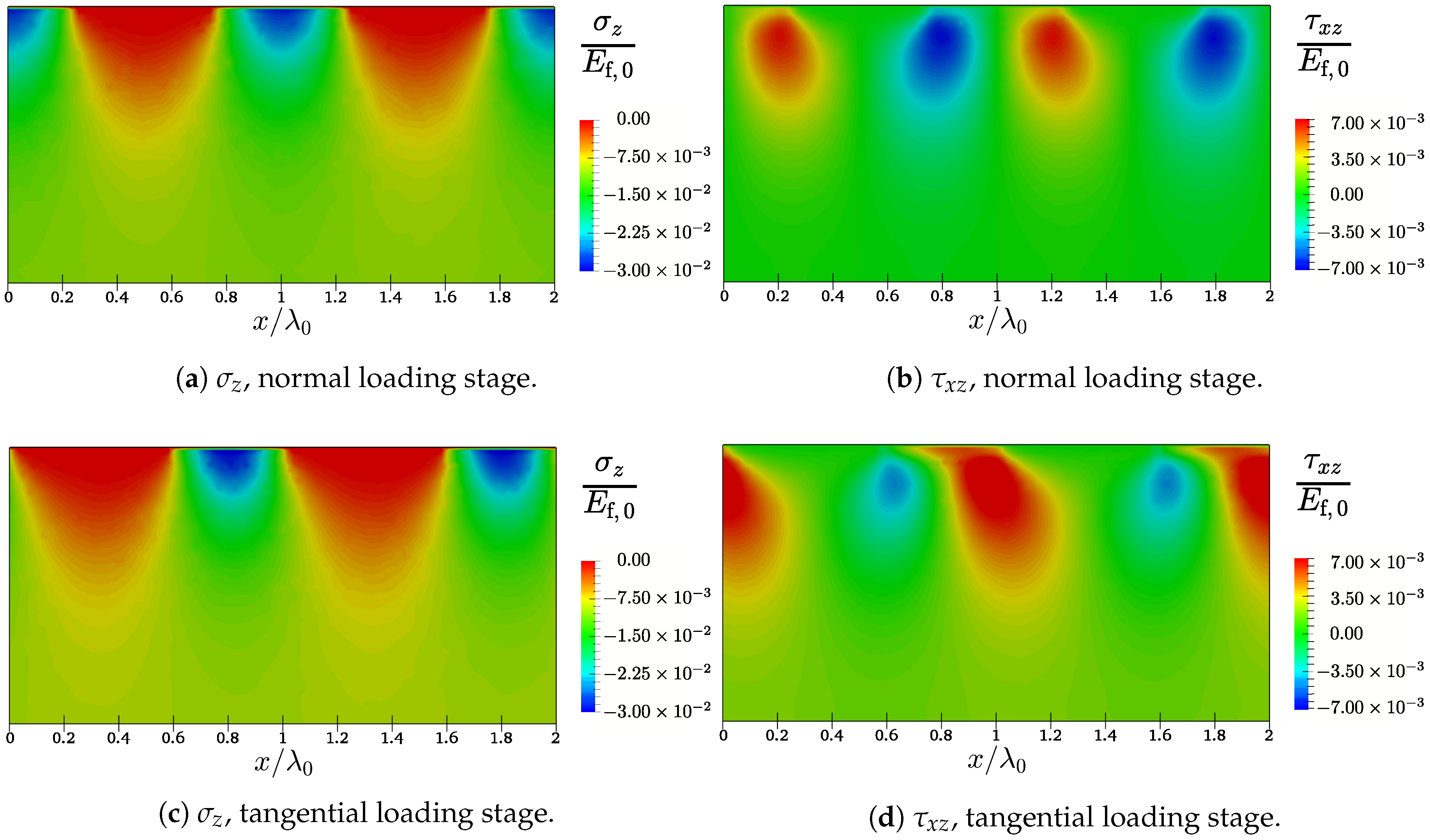
3.1. Bulk Stresses
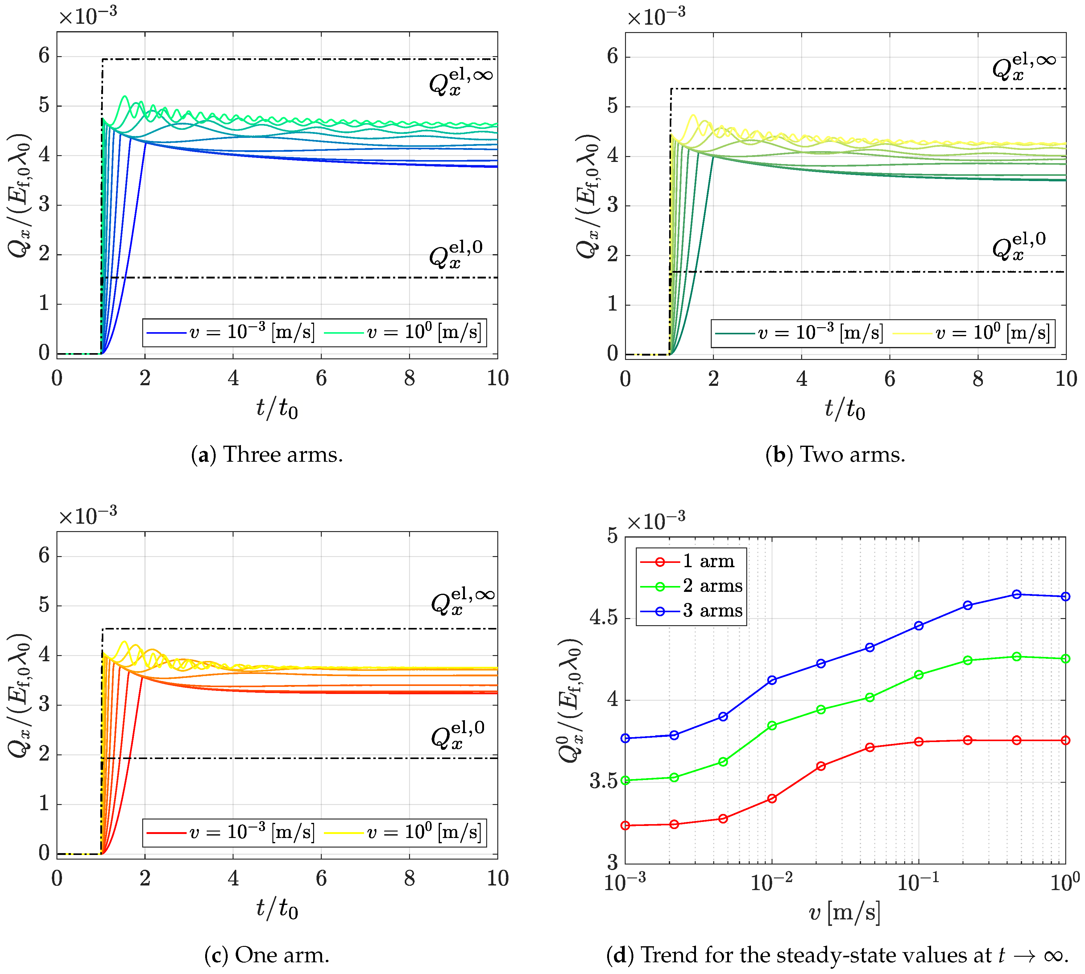
3.2. Interface Tractions
4. Conclusions
Author Contributions
Funding
Conflicts of Interest
Appendix A. Model Validation

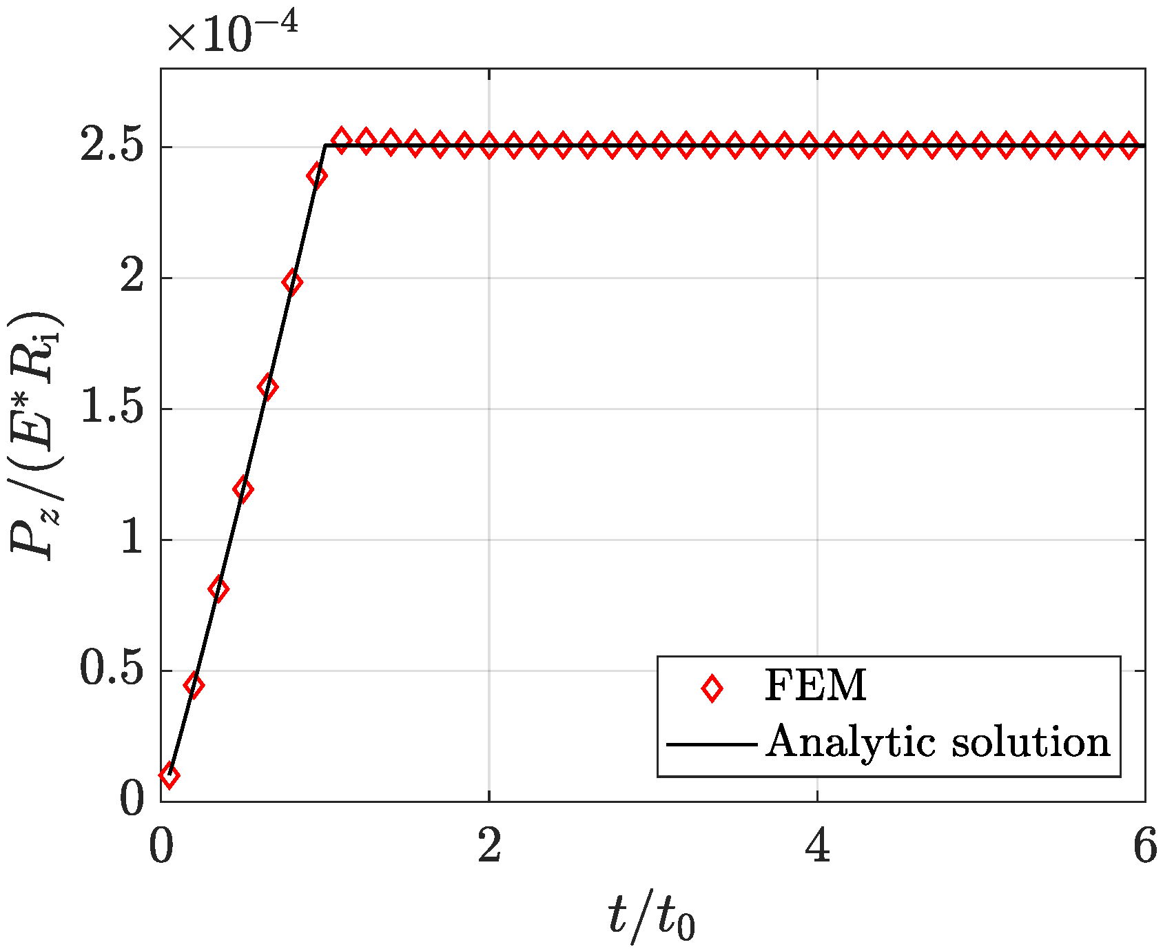
Appendix A.1. Evaluation of Normal Reaction Forces

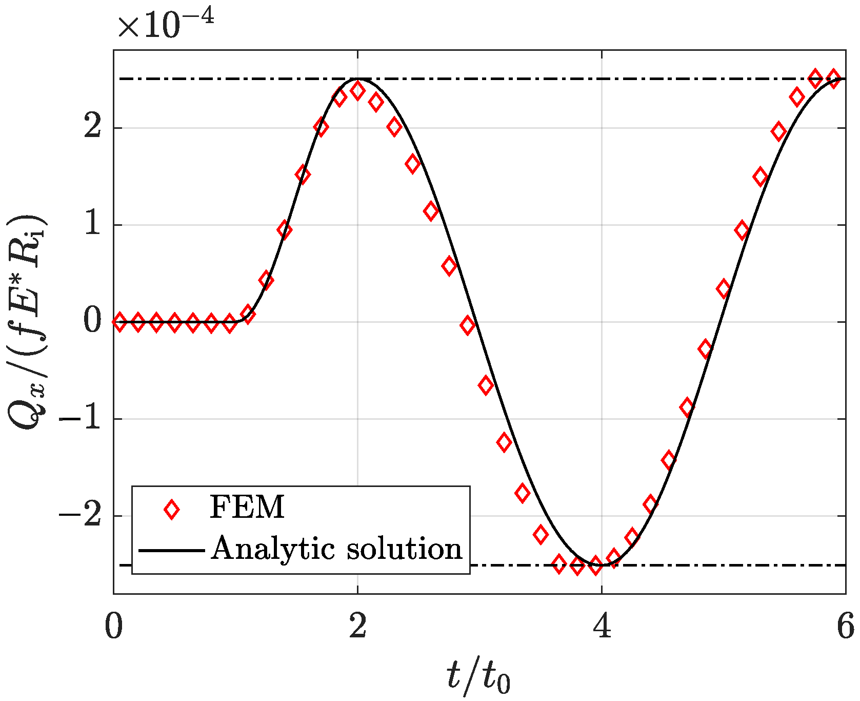
Appendix A.2. Evaluation of Tangential Reaction Forces

References
- Eitner, U. Thermomechanics of Photovoltaic Modules. Ph.D. Thesis, Zentrum für Ingenieurwissenschaften der Martin-Luther-Universität Halle-Wittemberg, Halle, Germany, 2011. [Google Scholar]
- Eitner, U.; Kajari-schröder, S.; Köntges, M.; Brendel, R. Non-linear mechanical properties of ethylene-vynil acetate (EVA) and its relevance to thermomechanics photovoltaic modules. In Proceedings of the 25th European Conference on Photovoltaic Solar Energy, Valencia, Spain, 6–10 September 2010; pp. 4366–4368. [Google Scholar]
- Paggi, M.; Kajari-Schröder, S.; Eitner, U. Thermomechanical deformations in photovoltaic laminates. J. Strain Anal. Eng. Des. 2011, 46, 772–782. [Google Scholar] [CrossRef]
- Paggi, M.; Sapora, A. An Accurate Thermoviscoelastic Rheological Model for Ethylene Vinyl Acetate Based on Fractional Calculus. Int. J. Photoenergy 2015, 2015. [Google Scholar] [CrossRef]
- Gagliardi, M.; Lenarda, P.; Paggi, M. A reaction-diffusion formulation to simulate EVA polymer degradation in environmental and accelerated ageing conditions. Sol. Energy Mater. Sol. Cells 2017, 164, 93–106. [Google Scholar] [CrossRef]
- Paggi, M.; Reinoso, J. A variational approach with embedded roughness for adhesive contact problems. Mech. Adv. Mater. Struct. 2020, 27, 1731–1747. [Google Scholar] [CrossRef]
- Paggi, M.; Bemporad, A.; Reinoso, J. Computational Methods for Contact Problems with Roughness. In Modeling and Simulation of Tribological Problems in Technology; Paggi, M., Hills, D., Eds.; Springer International Publishing: Cham, Switzerland, 2020; pp. 131–178. [Google Scholar] [CrossRef]
- Bonari, J.; Paggi, M.; Reinoso, J. A framework for the analysis of fully coupled normal and tangential contact problems with complex interfaces. 2020. submitted. [Google Scholar]
- Wriggers, P. Computational Contact Mechanics; Springer: Berlin/Heidelberg, Germany, 2006. [Google Scholar] [CrossRef]
- Zienkiewicz, O.; Taylor, R. The Finite Element Method for Solid and Structural Mechanics; Butterworth-Heinemann: Oxford, UK, 2000; Volume 2. [Google Scholar]
- Hills, D.; Nowell, D. Mechanics of Fretting Fatigue; Springer-Science + Business Media: Berlin/Heidelberg, Germany, 2020; pp. 20–24. [Google Scholar]
- Jäger, J. A New Principle in Contact Mechanics. J. Tribol. 1998, 120, 677–684. [Google Scholar] [CrossRef]


| n | ||||
|---|---|---|---|---|
| [–] | [Pa] | [–] | [–] | [s] |
| 1 | 568.498 | 0.421 | 0.579 | 0.817 |
| 2 | 674.606 | 0.306 | 0.398 | 0.212 |
| 0.296 | 2.458 | |||
| 3 | 749.386 | 0.254 | 0.310 | 0.102 |
| 0.226 | 0.545 | |||
| 0.210 | 4.104 |
| v |
|---|
Publisher’s Note: MDPI stays neutral with regard to jurisdictional claims in published maps and institutional affiliations. |
© 2020 by the authors. Licensee MDPI, Basel, Switzerland. This article is an open access article distributed under the terms and conditions of the Creative Commons Attribution (CC BY) license (http://creativecommons.org/licenses/by/4.0/).
Share and Cite
Bonari, J.; Paggi, M. Viscoelastic Effects during Tangential Contact Analyzed by a Novel Finite Element Approach with Embedded Interface Profiles. Lubricants 2020, 8, 107. https://doi.org/10.3390/lubricants8120107
Bonari J, Paggi M. Viscoelastic Effects during Tangential Contact Analyzed by a Novel Finite Element Approach with Embedded Interface Profiles. Lubricants. 2020; 8(12):107. https://doi.org/10.3390/lubricants8120107
Chicago/Turabian StyleBonari, Jacopo, and Marco Paggi. 2020. "Viscoelastic Effects during Tangential Contact Analyzed by a Novel Finite Element Approach with Embedded Interface Profiles" Lubricants 8, no. 12: 107. https://doi.org/10.3390/lubricants8120107
APA StyleBonari, J., & Paggi, M. (2020). Viscoelastic Effects during Tangential Contact Analyzed by a Novel Finite Element Approach with Embedded Interface Profiles. Lubricants, 8(12), 107. https://doi.org/10.3390/lubricants8120107