Dynamic Performances of Foil Bearing Supporting a Jeffcot Flexible Rotor System Using FEM

Abstract

Aerodynamic bearings have received considerable attention in recent decades and are increasingly being used in applications where high speed, low loads and high precision are required. Aerodynamic applications mainly concern auxiliary power units (APU) and air-conditioning machines (ACM). From the industrial point of view, the static and dynamic characteristics of these bearings rotating at very high speed must be determined. According to the literature, studies carried out on this type of bearing consider the elastic deformations of the foils due to the pressure generated in the air film. The linear approach is from time to time adopted for the prediction of the dynamic behavior of these bearings, which is not always justified. This paper aims to present a step towards a better mastery of the non-linear dynamic behavior of a flexible rotor-air bearing system. We will focus on finite element modeling (FEM) of the non-linear isothermal elasto-aerodynamic lubrication problem in the case of a radial bearing operating in a dynamic regime. We will present the effects of rotational speed, unbalance eccentricity, and rotor mass on the non-linear response of rigid and compliant bearings. We use a partitioned approach which treats fluid and structure as two computation domains solved separately; reducing the development time needed for a monolithic code which is difficult to manage when the geometries or the physical properties of the problem to be treated become complex.

1. Introduction

The development of foil bearings began in the early 1970s to provide rotational guidance of gas turbine shafts. One of the objectives was to validate their thermomechanical behavior at high temperatures [1,2]. Currently, the fields of application are more extensive but still concern the guidance of shafts rotating at very high speed, withstanding moderate loads and subjected to sometimes severe thermal stresses [3,4,5,6,7,8]. Some of them [3,5,9] consider the coupling between the bearing and the rotor with deformation of the sheets and friction between the sheets and the support using complex and numerically time-consuming approaches. Our aims in this paper are to present a first approach for this complex problem with a straightforward treatment of the non-linear dynamic behavior of a flexible rotor-air bearing system. For this purpose, we use finite element modeling (FEM) of the non-linear isothermal elasto-aerodynamic lubrication problem in a dynamic regime.

There are two families of foil bearing: Garett-type bearings and MITI-type bearings (Mohawk Innovative Technology Incorporated).

1.1. Garett’s Technology

The bearing consists of a sheath on which are hinged 8 to 12 sheets wound on each other. The assembly constitutes a deformable strap. Anchoring of these sheets is provided by means of a bar welded to the end of each sheet and housed in a notch on the sleeve, Figure 1.

The calculation of the clamping forces exerted by the sheets makes possible the starting torque evaluation. This step is used to initialize the iterative calculation process leading to the static characteristics determination. The proposed models are not simple because they must consider the friction forces between sheet–sheet, sheet–shaft and sheet–housing which are far from negligible. Although this technology is applied industrially in aerospace turbomachinery, it is now more often ruled out in favor of MITI technology that is more efficient and “simpler” to analyze.

1.2. Mohawk Innovative Technology Incorporated (MITI) Technology

The deformable structure of the bearing consists of a stack of smooth and corrugated sheets (stiffeners), Figure 2a [11,12]. The theoretical study of this type of foil bearing is much more complex than that of the spring bearings (Figure 2b). It must consider a solid mechanics analysis necessary to determine the deformation of the bearing when operating. However, structural models for solving the structural problem are generally simpler than those used for Garett technology. Indeed, the comparisons of the results obtained from the models with experimental work, on the load capacity, show that we can get rid of, as a first approximation, the friction sheets–stiffeners and stiffeners–sheath in the resolution of the elasto-aerodynamic problem [1].

Bearings using MITI-type technology have had several variations. Indeed, the number of lobes, upper leaves and stiffener sheets can be adapted according to the desired performance [2,11,12]. The first stage developed according to this technology (1st generation) consisted of a rigid sleeve on which are welded a corrugated sheet (stiffeners) and an upper sheet extending over the entire circumference of the bearing. This assembly of sheets provides both the profile of the bearing and its deformability, Figure 3. The proper implementation of the fixation of the deformable structure of the bearing (strip) imposes variation of its structural stiffness with the angular position of the considered point. Subsequently, lobed bearings appeared, generally in three sectors. As for single-lobed bearings, the deformable structure has a stiffness that varies along the circumference. This type of bearing has good dynamic characteristics. Experimental studies, and in particular the analysis of rotor displacements at the level of the bearings, highlight a privileged direction of rotation [1]. The best stability is obtained by choosing a direction of rotation of the free part towards the fixed part of the deformable structure.

The level of stability of these lobed bearings is generally high even for moderate loads. Among the technologies used successfully, one of them stands out with particularly interesting results and simple modeling: the technology of MITI-type stacking bearings [13]. Numerous numerical and experimental studies are interested in the static and dynamic characteristics of this type of bearings [4,5,6,7,8,14]. These papers focused on two areas:

• In-depth research on the tribological phenomena related to stopping and starting [15]; dry friction that occurs during these phases is the main cause of deterioration of the bearings. The state of the surfaces and the materials in contact have a decisive influence in the phenomena involved;
• The development of a theoretical model allowing a precise simulation of the elasto-aerodynamic or even thermo-elasto aerodynamic performance of the bearing [2,16,17,18,19]

We will focus here mainly on the second line of research based on the following assumptions:

-

Isothermal operating regime;

-

The fluid, which is air, is thermodynamically assimilated to a perfect gas;

-

Coulomb friction between the different solid parts is neglected.

2. The Basic Equations

2.1. Reynolds Equation

The general equations of aerodynamic lubrication allow us, in view of the geometrical and kinematic conditions, to determine the characteristics of the flow of thin film air and particularly its aerodynamic lift [20]. Under thin-film assumptions, one can obtain a generalized Reynolds equation governing the flow inside the contact. In a bearing where the shaft is rotated in a fixed bore (Figure 4), the radial clearance $C$ is very small compared to the radius $R$ of the bearing (or the shaft). We can neglect the curvature of the film and develop the bearing in its circumferential direction. Under these conditions, the surface of the housing is merged with the plane $\left(O,x,z\right)$ of the reference frame. If the axes of the shaft and the bearing are parallel, the surface of the shaft is presented such that $y=h\left(x,z,t\right)$. In this case, the Reynolds equation takes the following form:

$$\frac{\partial }{\partial x}\left(\frac{\rho h^3}{\mu }\frac{\partial p}{\partial x}\right)+\frac{\partial }{\partial z}\left(\frac{\rho h^3}{\mu }\frac{\partial p}{\partial z}\right)=6U_2\frac{\partial \left(\rho h\right)}{\partial x}+12\frac{\partial \left(\rho h\right)}{\partial t}\mathrm{in}\left(\mathrm{D}\right)$$

(1)

By replacing $x$ by $R\theta$, we obtain the following form written in cylindrical coordinates:

$$\frac{1}{R^2}\frac{\partial }{\partial \theta }\left(\frac{\rho h^3}{\mu }\frac{\partial p}{\partial \theta }\right)+\frac{\partial }{\partial z}\left(\frac{\rho h^3}{\mu }\frac{\partial p}{\partial z}\right)=6\omega \frac{\partial \left(\rho h\right)}{\partial \theta }+12\frac{\partial \left(\rho h\right)}{\partial t}$$

(2)

$\omega$ is the angular velocity of the shaft and $\theta$ the circumferential coordinate of the bearing.

The air is considered as a perfect gas with the following equation of state:

$$p=\rho \Re T$$

(3)

where $\Re$ is the perfect gas constant.

Given the equation of state (3) and assuming that $\Re$ and $T$ are constant, the compressible Reynolds equation is written for an iso-viscous fluid as follows:

$$\frac{1}{R^2}\frac{\partial }{\partial \theta }\left(p{h}^3\frac{\partial p}{\partial \theta }\right)+\frac{\partial }{\partial z} \left(p{h}^3\frac{\partial p}{\partial z}\right)=6\mu \omega \frac{\partial \left(ph\right)}{\partial \theta }+12\mu \frac{\partial \left(ph\right)}{\partial t}$$

(4)

The boundary conditions required are:

$$\{\begin{array}{c}p\left(\theta =0,z\right)=p_a \\ p\left(\theta =2\pi ,z\right)=p_a\end{array}\{\begin{array}{c}p\left(\theta ,z=-L/2\right)=p_a\\ p\left(\theta ,z=+L/2\right)=p_a\end{array}$$

(5)

where $p_a$ is the atmospheric pressure.

In the form (4), the Reynolds equation is strongly non-linear, and its resolution cannot be performed analytically.

In dimensionless form, Equations (4) and (5) become:

$$\frac{\partial }{\partial \theta }\left(\tilde{p}{\tilde{h}}^3\frac{\partial \tilde{p}}{\partial \theta }\right)+\lambda \frac{\partial }{\partial \tilde{\mathfrak{z}}}\left(\tilde{p}{\check{h}}^3\frac{\partial \tilde{p}}{\partial \tilde{z}}\right)=\mathsf{\Lambda }\frac{\partial }{\partial \theta }\left(\tilde{p}\tilde{h}\right)+2\mathsf{\Lambda }\frac{\partial }{\partial \tilde{t}}\left(\tilde{p}\tilde{h}\right)$$

(6)

and

$$\{ \begin{array}{c}\tilde{p} \left(\theta =0,\tilde{z}\right)=1 \\ \tilde{p}\left(\theta =2\pi ,\tilde{z}\right)=1 \end{array}\tilde{p}\left(\theta ,\tilde{z}=\pm 1/2\right)=1$$

(7)

With $\tilde{p}=p/p_a, \tilde{h}=h/C, \tilde{z}=z/L, \tilde{t}=\omega t et \lambda ={\left(R/L\right)}^2$

$\mathsf{\Lambda }=\frac{6\mu \omega {\left(R/C\right)}^2}{P_a}\mathrm{Representing}\mathrm{the}\mathrm{compressibility}\mathrm{number}.$

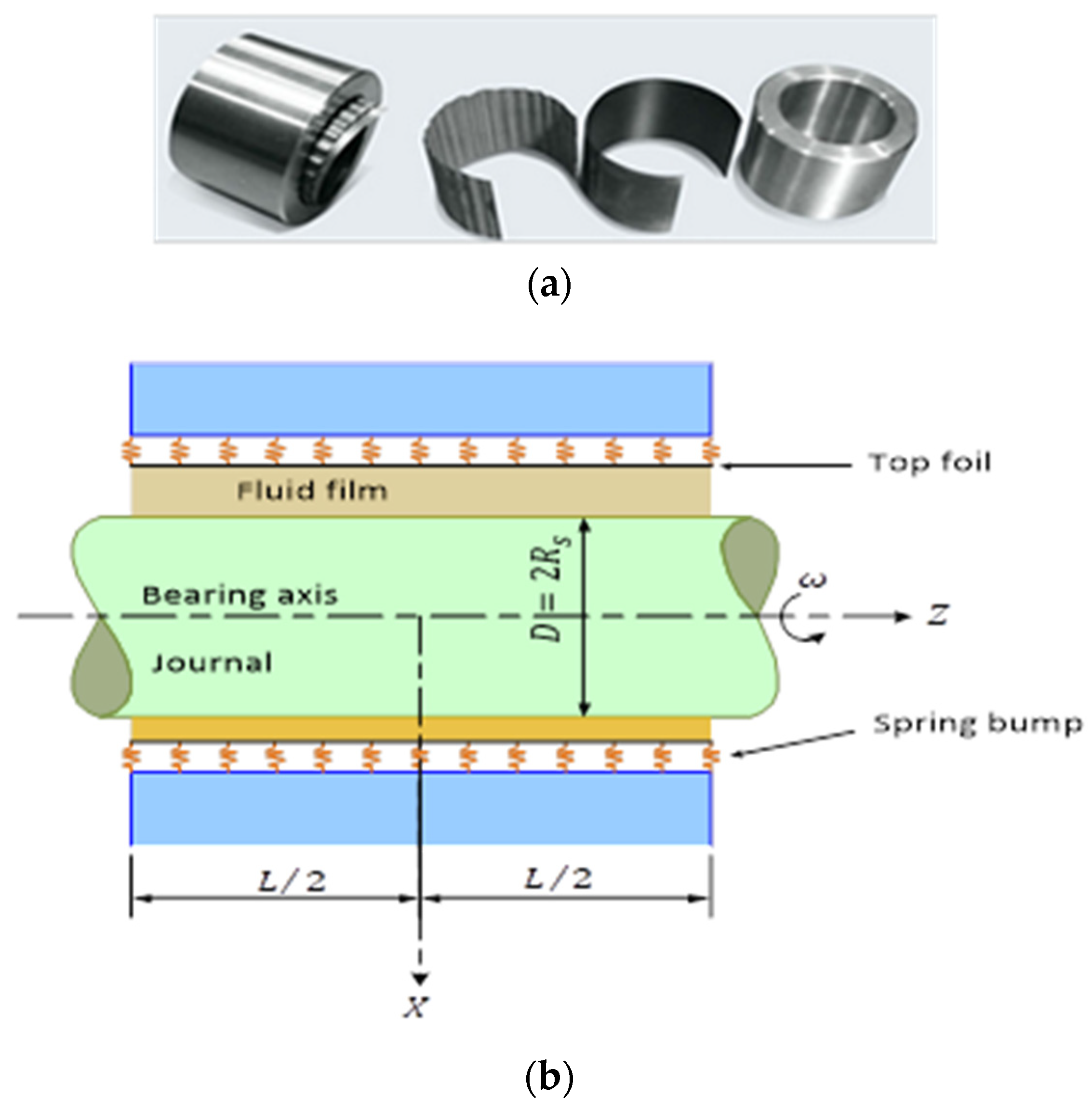
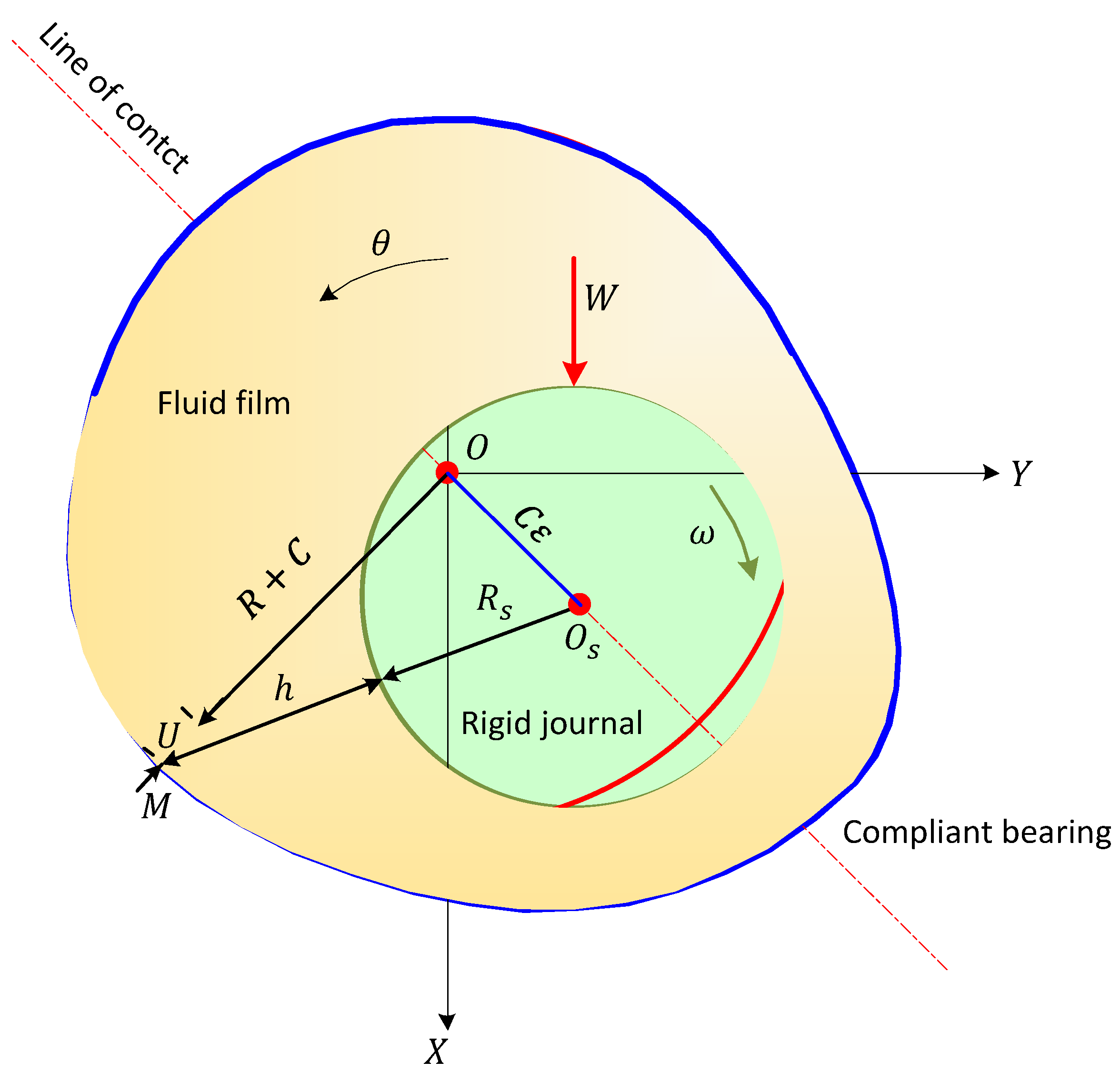
2.2. Equation of the Film Geometry in the Case of a Foil Bearing

Figure 5 shows schematically a compliant aerodynamic bearing. The representation of the rigid bearing is defined by the circle of radius $\left(R+C\right)$. The origin of the $X$, $Y$ and $Z$ frame is located at the center of the rigid (non-deformable) bearing $O_b$.

The circumferential coordinate $\theta$ is measured from the O_bX axis. The shaft is considered rigid and is subjected to a constant angular rotation speed $\omega$ along the $Z$ axis. The instantaneous position of the geometric center of the bearing $e\left(t\right)=C\epsilon \left(t\right)$ is defined by the running eccentricity and the static attitude angle $\varphi \left(t\right)$ with respect to the Cartesian coordinates $X\left(t\right)$, $Y\left(t\right)$.

The radial clearance of the bearing when the shaft and the bearing are coaxial in the case of a rigid bearing is defined by $C$, and the thickness of the film in the case of radial deformation $U\left(\theta ,z,t\right)$ of the top sheet is represented by $h_{}$ with:

$$h\left(t\right)=C\left(1+\epsilon \left(t\right)\cos \left(\theta -\phi (t\right)\right)+U\left(\theta ,z,t\right)$$

(8)

or

$$h{\left(\theta ,z,t\right)}_{ }=C+X\left(t\right)\cos \theta +Y\left(t\right)\sin \theta +U\left(\theta ,z,t\right)$$

(9)

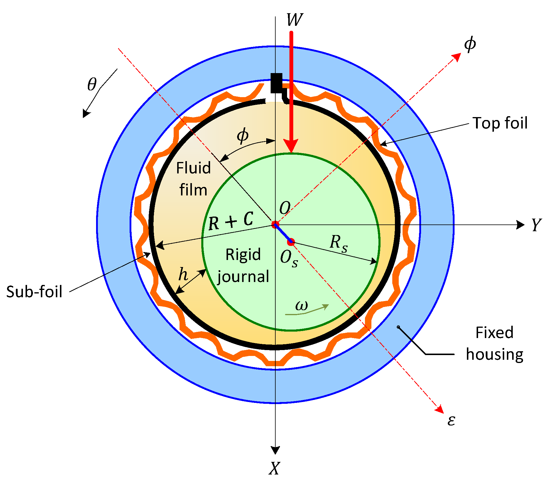
2.3. Expression of the Radial Deformation U

As a first approximation, the compliance of corrugated sheets can be calculated using the simplified model from Heshmat [11,12], Figure 6. A more complete FE-type approach gives more realistic results when non-linearities are important. These non-linearities come essentially from the specific characteristics of the sheets [1] but as a first approximation to obtain information on the bearing behavior an approach of this kind is enough [21]. Heshmat’s approach is used because of its simplicity. A more complete and complex approach exists (beam and shell by FE, see [1,21]). We want here to focus on the comparison between rigid and deformable structure in dynamic regime without spending too much time for computer calculations. We have:

$$h_{ }=C+e\cos \left(\theta -\varphi \right)+K\left(p-p_a\right)$$

(10)

with:

$$K=\frac{2s}{E} {\left(\frac{1}{t_b}\right)}^3\left(1-v²\right)$$

(11)

where $E$ and $v$ are respectively the Young’s modulus and the Poisson’s ratio of the material constituting the sheets and with:

• e: is the eccentricity such as $e=|\overrightarrow{O_b{O}_j}|.$
• $C$: bearing radial clearance, $C=R-R_s.$
• $\theta$: the circumferential coordinate measured from the axis $OX$.

In dimensionless form, Equation (10) becomes,

$$h_{ }=C+e\cos \left(\theta -\varphi \right)+K\left(p-p_a\right)$$

(12)

$$\widetilde{h }=\frac{h}{C}=1+\epsilon \cos \left(\theta -\varphi \right)+ \alpha \left(\tilde{p}-1 \right)$$

(13)

where $\epsilon =e/C$ the relative eccentricity, and $\alpha$ being the dimensionless compliance number defined by the following relation:

$$\alpha = \frac{2P_{a }. s}{EC} {\left(\frac{\ell }{t_b}\right)}^3\left(1-v²\right)$$

(14)

3. Resolution of Compressible Reynolds Equation under Transient Conditions

For an instantaneous position of the bearing shaft center defined by the Cartesian coordinates $X\left(t\right)$ and $Y\left(t\right)$, the transient compressible Reynolds equation is written taking into account the transient term appearing in the right-hand side of the equation:

$$\frac{\partial }{\partial \theta }\left(\tilde{p}{\tilde{h}}^3\frac{\partial \tilde{p}}{\partial \theta }\right)+\lambda \frac{\partial }{\partial \tilde{z}}\left(\tilde{p}{\tilde{h}}^3\frac{\partial \tilde{p}}{\partial \tilde{z}}\right)=\mathsf{\Lambda }\frac{\partial }{\partial \theta }\left(\tilde{p}\tilde{h}\right)+2\mathsf{\Lambda }\frac{\partial }{\partial \tilde{t}}\left(\tilde{p}\tilde{h}\right)$$

(15)

This equation has to be solved in $\tilde{D}=\left(0,2\pi \right)\times \left(-1/2,1/2\right).$

with

$$\tilde{h}\left(\widetilde{\theta ,}\tilde{z},\tilde{t}\right)=1+\tilde{X}\left(t\right)cos\theta +\tilde{Y}\left(t\right)sin\theta +\alpha \left(\tilde{p}\left(\widetilde{\theta ,}\tilde{z},\tilde{t}\right)-1\right)$$

(16)

and $\left(\tilde{X},\tilde{Y}\right)=\left(X,Y\right)/C.$

Using the Galerkin variational approach the integral form associated with Equation (21) is [22,23]:

$$\tilde{W}\left(\tilde{p}\right)={{\displaystyle \iint }}_{\tilde{D}}^{}\delta \tilde{p}\left[\frac{\partial }{\partial \theta }\left(\tilde{p}{\tilde{h}}^3\frac{\partial \tilde{p}}{\partial \theta }\right)+\lambda \frac{\partial }{\partial \tilde{z}}\left(\tilde{p}{\tilde{h}}^3\frac{\partial \tilde{p}}{\partial \tilde{z}}\right)-\mathsf{\Lambda }\frac{\partial }{\partial \theta }\left(\tilde{p}\tilde{h}\right)-2\mathsf{\Lambda }\frac{\partial }{\partial \tilde{t}}\left(\tilde{p}\tilde{h}\right)\right]d\tilde{D}=0$$

(17)

Either after integration by parts taking into account the boundary conditions $(\tilde{p} \left(\theta ,\tilde{z},\tilde{t}\right)=1$ at the frontier of the domain $\tilde{D}$):

$$\tilde{W}\left(\tilde{p}\right)={{\displaystyle \iint }}_{\tilde{D}}^{}\left[\tilde{p}{\tilde{h}}^3\left(\frac{\partial \delta \tilde{p}}{\partial \theta }\frac{\partial \tilde{p}}{\partial \theta }+\lambda \frac{\partial \delta \tilde{p}}{\partial \tilde{z}}\frac{\partial \tilde{p}}{\partial \tilde{z}}\right)-\mathsf{\Lambda }\tilde{p}\check{h}\frac{\partial \delta \tilde{p}}{\partial \theta }+2\mathsf{\Lambda }\delta \tilde{p}\frac{\partial }{\partial \tilde{t}}\left(\tilde{p}\tilde{h}\right)\right]d\tilde{D}=0$$

(18)

or:

$${{\displaystyle \int }}_{-1/2}^{1/2}{{\displaystyle \int }}_0^{2\pi }\left[\tilde{p}{\tilde{h}}^3\left(\frac{\partial \delta \tilde{p}}{\partial \theta }\frac{\partial \tilde{p}}{\partial \theta }+\lambda \frac{\partial \delta \tilde{p}}{\partial \tilde{z}}\frac{\partial \tilde{p}}{\partial \tilde{z}}\right)-\mathsf{\Lambda }\tilde{p}\tilde{h}\frac{\partial \delta \tilde{p}}{\partial \theta }+2\mathsf{\Lambda }\delta \tilde{p} \tilde{p}\frac{\partial \tilde{h}}{\partial \tilde{t}}+2\mathsf{\Lambda }\delta \tilde{p}\tilde{h}\frac{\partial \tilde{p}}{\partial \tilde{t}}\right]d\tilde{D}=0$$

(19)

with:

$$\begin{gathered} \frac{\partial \tilde{h}}{\partial \tilde{t}}=\tilde{h}\prime =\tilde{X}\prime cos\theta +\tilde{Y}\prime sin\theta +\alpha \tilde{p}\prime \\ \tilde{p}\prime =\frac{\partial \tilde{p}}{\partial \tilde{t}}, \tilde{X}\prime =\frac{d\tilde{X}}{d\tilde{t}} et \tilde{Y}\prime =\frac{d\tilde{Y}}{d\tilde{t}} \end{gathered}$$

(20)

Given Equation (20), Equation (19) becomes:

$$\begin{gathered} {{\displaystyle \int }}_{-1/2}^{1/2}{{\displaystyle \int }}_0^{2\pi }\tilde{p}{\tilde{h}}^3\left(\frac{\partial \delta \tilde{p}}{\partial \theta } \frac{\partial \tilde{p}}{\partial \theta }+\lambda \frac{\partial \delta \tilde{p}}{\partial \tilde{z}} \frac{d\tilde{p}}{\partial \tilde{z}}\right)d\theta d\tilde{z}+{{\displaystyle \int }}_{-1/2}^{1/2}{{\displaystyle \int }}_0^{2\pi }2\mathsf{\Lambda }\delta \tilde{p}\left(\tilde{h}+\alpha \tilde{p}\right)\tilde{p}\prime d\theta d\tilde{z} \\ ={{\displaystyle \int }}_{-1/2}^{1/2}{{\displaystyle \int }}_0^{2\pi }\mathsf{\Lambda } \tilde{p}\tilde{h}\frac{\partial \delta \tilde{p}}{\partial \theta }d\theta d\tilde{z}-\underset{-1/2}{\overset{1/2}{{\displaystyle \int }}}\underset{0}{\overset{2\pi }{{\displaystyle \int }}}2\mathsf{\Lambda }\delta \tilde{p}\tilde{p}\left(\tilde{X}\prime cos+\tilde{Y}\prime sin\theta \right)d\theta d\tilde{z} \end{gathered}$$

(21)

which leads after discretization [18,24] to the following first order differential system:

$$\left[\complement \left({\mathbb{P}}_n,\tilde{t}\right)\right]\left\{\mathbb{P}{\prime }_n\left(\tilde{t}\right)\right\}+\left[K \left({\mathbb{P}}_n,\tilde{t}\right)\right]\left\{{\mathbb{P}}_n\left(\tilde{t}\right)\right\}= \left\{F\left({\mathbb{P}}_n,\tilde{t})\right)\right\}$$

(22)

The transient Reynolds equation is then solved by using the implicit Euler method. The implicit Euler method is well known and is unconditionally stable. We wanted to be sure of not having a diverging process from the deformations of the structure.

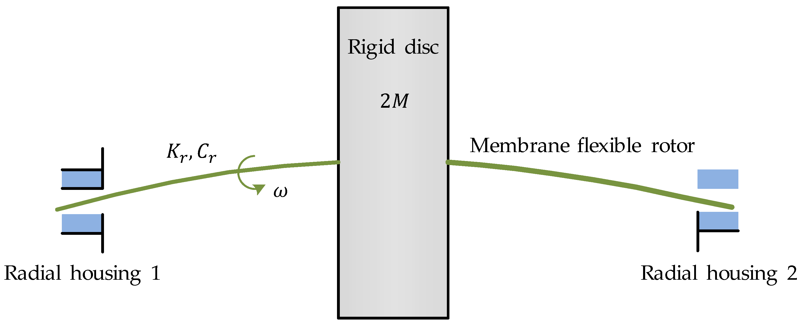
4. Equations of Rotor Motion

The rotor of a rotating machine is a very important element with a role to transmit or transform power [24]. In many applications, it is supported by bearings that should not be considered as passive elements but as elements that play a significant role in the dynamic behavior of the shaft line on its critical speeds and stability.

Balance of External Forces

The external forces acting on the rotor are:

• weight of the rotor;
• external dynamic forces;
• aerodynamic forces generated in the air film.

The shaft line can be represented by a flexible rotor (Jeffcott rotor system) of mass $2m$, stiffness $2K_r$ and damping $2C_r$ supported symmetrically by 2 identical foil bearings Figure 7. Each bearing is assigned a mass $M$ of the rotor, a stiffness $K_r$ and a damping $C_r$ of the rotor, a static load ${\overrightarrow{W}}_0=W_0\overrightarrow{X}$, a dynamic load $\overrightarrow{W}\left(t\right)$ and a synchronous excitation due to an unbalance characterized by its eccentricity $e_b$ with $M{e}_b{\omega }^2$ magnitude. When balancing is perfect, the center of inertia $G$ of the shaft is the same as its geometric center.

For a non-linear analysis we must apply the fundamental principle of dynamics to the rotor-bearing system which gives:

$$\{\begin{array}{c}M\ddot{X}+C_r\dot{X}+K_{r}X=W_0+W_X\left(t\right)+M{e}_b{\omega }^2\cos \omega t+F_X\left(X,Y,\dot{X},\dot{Y}\right)\\ M\ddot{Y}+C_r\dot{Y}+K_{r}Y=W_Y\left(t\right)+M{e}_b{\omega }^2\sin \omega t+F_Y\left(X,Y,\dot{X},\dot{Y}\right)\end{array}$$

(23)

where $X\left(t\right)$ et $Y\left(t\right)$ represent the instantaneous coordinates of the shaft center, i.e.,

$$\overrightarrow{O{O}_s}=\left\{\begin{array}{c}X\left(t\right)\\ Y\left(t\right)\end{array}\right\}=\left\{\begin{array}{c}C\epsilon \left(t\right)\cos \varphi \left(t\right)\\ C\epsilon \left(t\right)\sin \varphi \left(t\right)\end{array}\right\}$$

and $\left\{\begin{array}{c}{F}_x\left(t\right)\\ F_y\left(t\right)\end{array}\right\}={{\displaystyle \int }}_{-1/2}^{1/2}p\left(\theta ,z,t\right)\left\{\begin{array}{c}\cos \theta \\ \sin \theta \end{array}\right\}R d\theta dz$ are the components of the aerodynamic action calculated from the pressure field obtained by integrating the compressible Reynolds Equation (15).

For numerical processing, it is better to write Equations (23) in the following dimensionless form:

$$\left[\begin{array}{cc}M& 0\\ 0& M\end{array}\right]\left\{U″\right\}+\left[\begin{array}{cc}{\tilde{C}}_r& 0\\ 0& {\tilde{C}}_r\end{array}\right]\left\{U\prime \right\}+\left[\begin{array}{cc}{\tilde{K}}_r& 0\\ 0& {\tilde{K}}_r\end{array}\right]\left\{U\right\}=\left\{\begin{array}{c}{\tilde{W}}_0+{\tilde{W}}_X\left(\tilde{t}\right)+M{\epsilon }_b\cos \left(\tilde{t}\right)+{\tilde{F}}_X\left(\tilde{X},\tilde{Y},\widetilde{X\prime },\widetilde{Y\prime }\right)\\ {\tilde{W}}_Y\left(\tilde{t}\right)+M{\epsilon }_b\sin \left(\tilde{t}\right)+{\tilde{F}}_Y\left(\tilde{X},\tilde{Y},\widetilde{X\prime },\widetilde{Y\prime }\right) \end{array}\right\}$$

(24)

with:

$$\begin{gathered} M=\frac{mC{\omega }^2}{p_{a}RL}, {\tilde{C}}_r=\frac{C_{r}C\omega }{p_{a}RL}, {\tilde{K}}_r=\frac{K_{r}C}{p_{a}RL}, {\epsilon }_b=\frac{e_b}{C} , \tilde{t}=\omega t \\ \left({\tilde{W}}_0,{\tilde{W}}_X,{\tilde{W}}_Y,{\tilde{F}}_X,{\tilde{F}}_Y\right)=\frac{\left(W_0,W_X,W_Y,F_X,F_Y\right)}{p_{a}RL} \end{gathered}$$

with:

$$\begin{gathered} (·)\prime =\frac{d}{d\tilde{t}}\left(·\right)=\frac{d\left(·\right)}{d\tilde{t}}\frac{dt}{d\tilde{t}}=\frac{1}{\omega }\frac{d}{dt}\left(·\right) \\ \left\{U\right\}=\left\{\begin{array}{c}\tilde{X}\\ \tilde{Y}\end{array}\right\}, \left\{U\prime \right\}=\left\{\begin{array}{c}\tilde{X}\prime \\ \tilde{Y}\prime \end{array}\right\} et \left\{U″\right\}=\left\{\begin{array}{c}\tilde{X}″\\ \tilde{Y}″\end{array}\right\} \end{gathered}$$

With a small displacements hypothesis in the neighborhood of the equilibrium position, we cannot predict correctly the behavior of a rotor beyond the stability threshold or under high dynamic loads [26]. It is then necessary to couple the non-linear motion equations of the rotor (24) to the transient Reynolds Equation (15). The coupling between the rotor motion equations and the Reynolds equation is undertaken through the components of the aerodynamic forces F_X and F_Y. The Newmark method is well known for its robustness. We prefer to develop our own models rather than using black boxes whose involvement is difficult to assess when the numerical process is not working. To solve Equation (24), we use the Newmark numerical scheme [18]:

$${\tilde{X}}^{\prime }\left(\tilde{t}+\mathsf{\Delta }\tilde{t}\right)=\tilde{X}\prime \left(\tilde{t}\right)+\mathsf{\Delta }\tilde{t}\left[\left(1-a\right)\tilde{X}″\left(\tilde{t}\right)+a.\tilde{X}″\left(\tilde{t}+\mathsf{\Delta }\tilde{t}\right)\right]$$

Numerical approaches to solve this fluid–structure interaction problem can be classified into two methods, monolithic and partitioned. The monolithic approach treats the dynamics of fluids and structures in the same mathematical model to form a single equation for the whole problem [27]. The equations of the fluid and the structure are solved simultaneously with a single calculation code. The conditions at the interface between the fluid and the solid are implicitly solved, which guarantees unconditional stability. In general, monolithic schemes are precise and stable, but very expensive in terms of calculation. In addition, a monolithic approach is neither easy to implement, nor to implement and evolve. When the geometries or the physical properties of the problem to be treated become complex, this type of method is no longer possible since each medium requires numerical computation procedures specific approach that the monolithic approach does not exploit. The partitioned approach treats fluid and structure as two computation domains that can be solved separately, with their own discretization and numerical algorithm. The conditions at the interface are explicitly solved to share information between fluid and structural solutions. A strong reason for using this approach is the possibility to integrate the algorithms already available for the resolution of the fluid and the structure and thus to reduce the development times of a monolithic code. The use of numerical algorithms that have been validated and used to solve many problems makes it possible to benefit from the robustness of the two parts. Here, we used a partioned approach.

5. Parametric Studies

Data

The geometrical and elastic characteristics as well as the operating conditions of the air bearing are shown in

Table 1. Geometrical and material characteristics.

Parameter	Symbol	Value	Unit (SI)
Radius	$R$	50 × 10−3	$\mathrm{m}$
Lenght	$L$	110 × 10−3	$\mathrm{m}$
Radial clearance	$C$	30 × 10−6	$\mathrm{m}$
Bump foil thickness	$t_b$	0.1016 × 10−3	$\mathrm{m}$
Bump pitch	$s$	4.572 × 10−3	$\mathrm{m}$
Bump length	$l$	3.556 × 10−3	$\mathrm{m}$
Young modulus	$E$	∞ (rigid) 207	$\mathrm{GPa}$
Poisson ratio	$\nu$	0:30

and

Table 2. Running conditions.

Parameter	Symbol	Value	Unit (SI)
Rotor mass assigned to bearing	$m$	10.5	$\mathrm{Kg}$
Rotational speed	$N$	12,300	$\mathrm{rpm}$
Atmospheric pressure	$Pa$	1.013 × 105	$\mathrm{Pa}$
Unbalance eccentricity	$e_b$	0	$\mathrm{M}$
Rotor stiffness assigned to bearing	$K_r$	2.03 × 105 2.03 × 106	$\mathrm{N}/\mathrm{m}$
Rotor damping assigned to bearing	$C_r$	10103	$\mathrm{N}·\mathrm{s}/\mathrm{m}$

. The different calculations were performed using the finite element mesh data

Table 3. Mesh information.

Parameter	Value
Element of approximation	Quadrilateral bilinear C° 4 nodes
Number of elements in circumferential and axial directions (half bearing)	$N_{\theta }=30,N_z=10$

.

6. Results and Discussion

All the units when not specified are in microns. Figure 8a–c show the trajectories of the center of the rotor calculated for two values of rotational speed $N=\mathrm{12,300} \mathrm{rpm}$ and $N=\mathrm{30,000} \mathrm{rpm}$ in the case of a rigid air bearing and a bearing with compliant foils. The rotor is supposed to be perfectly balanced ($e_b=0$) and we start the calculation from the same initial position. In the rigid case, the center of the rotor moves rapidly to its operating position (equilibrium position) after a certain number of revolutions of the rotor. On the other hand, when the elasticity of the foils is taken into account, the center of the rotor describes an orbit. The pressure generated in the film in the rigid case is higher and contributes to a faster movement towards the equilibrium position. Note that the result obtained in the rigid case is in good agreement with that published in the literature [4].

In Figure 9 when the speed increases ($N\ge \mathrm{30,000} \mathrm{rpm}$), the bearing becomes unstable and the center of the shaft then reaches extremely high eccentricities that can exceed the value of the initial radial clearance especially in the case of the compliant bearing. It is concluded that the theory of aerodynamic lubrication that neglects the elastic deformations does not correctly predict the dynamic behavior of the bearing in terms of response and stability. On the other hand, we note that the orbit computed for a compliant bearing does not have a quite elliptical form like that predicted by the linear theory.

We were also interested in studying the influence of the unbalance eccentricity on the dynamic response of the air bearing. For this, we performed three simulations in the case of an unbalanced rotor by using unbalance eccentricities $e_b=1\mathsf{\mu }\mathrm{m}$, $e_b= 6 \mathsf{\mu }\mathrm{m}$ and $e_b= 8 \mathsf{\mu }\mathrm{m}$ Figure 10. It is clearly observed that the size of the orbit described by the center of the shaft increases with the eccentricity of unbalance both in the rigid case and in the compliant case. It should be emphasized that the results obtained in the rigid case and compliant are totally different.

Figure 11 and Figure 12 show the trajectories and the evolutions of the center of the shaft displacement in the X direction as a function of time for different values of mass rotor, for a rotational speed $N=\mathrm{12,300}\mathrm{rpm}$ and an unbalance eccentricity $e_b=1 \mathsf{\mu }\mathrm{m}$. Calculations were made for a rigid bearing and a compliant bearing. The results obtained in the rigid case show that the size of the orbit decreases with the mass of the rotor while keeping the same shape. On the other hand, taking into account the elasticity of the foils significantly influences the shape of the orbits. One can observe significant attenuation of the amplitude of the trajectory during the increase of the mass ([1]). Concerning the consequences on the temporal and frequency behavior, there is a disappearance of the whirl during the increase of the mass of the rotor. The sub synchronous frequencies are of less amplitude and less numerous. Increasing the mass moves the operating point towards the stable region, a known phenomenon in linear analysis. At 5 kg, we observe the appearance of the whirl which disappears at 7 kg and 10.5 kg. Indeed, by increasing the weight, the air film becoming stiffer no longer excites the rotor at this speed. However, at 5 kg a whirl phenomenon corresponds to the excitation of the cylindrical mode by the structure.

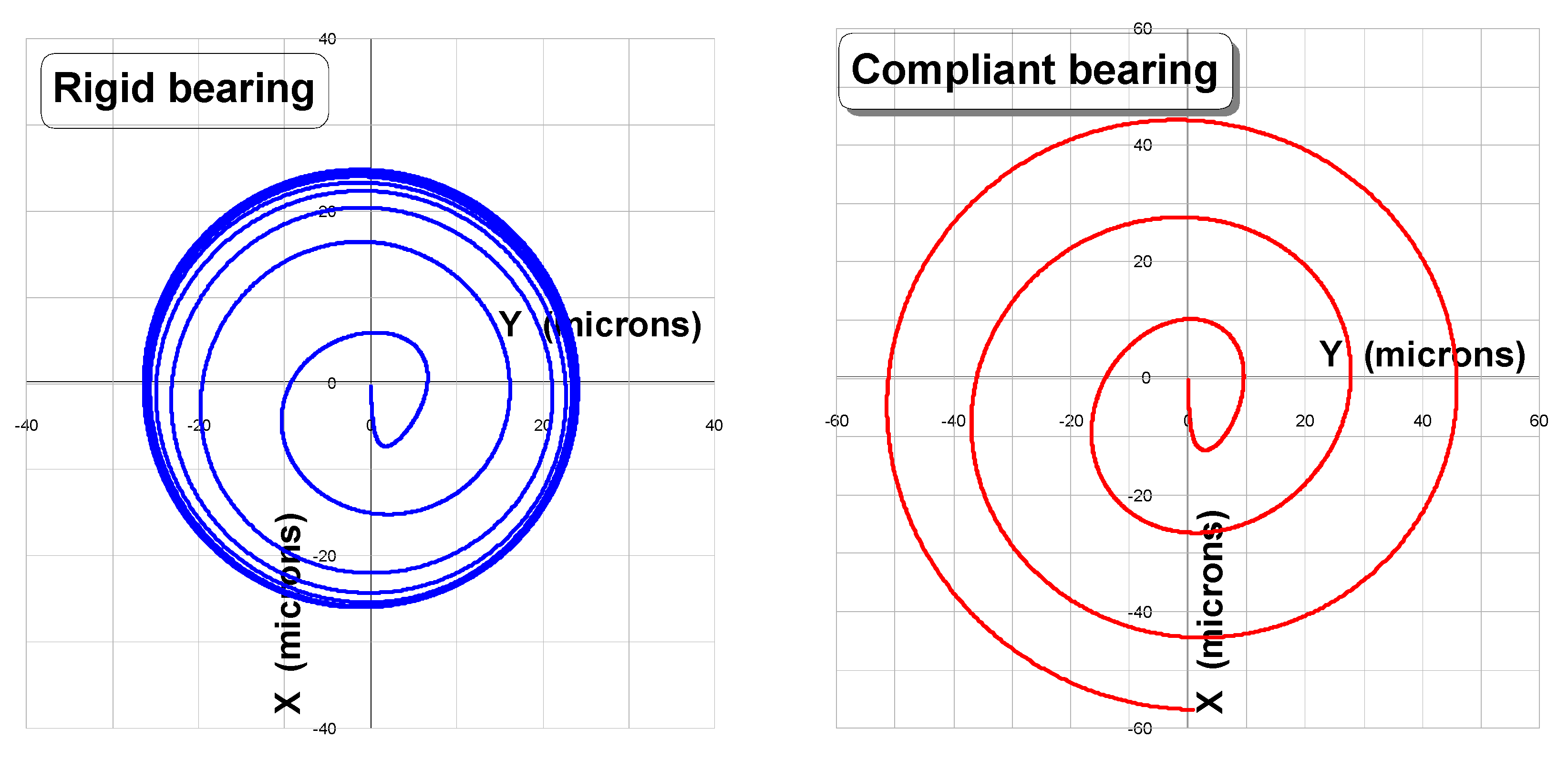
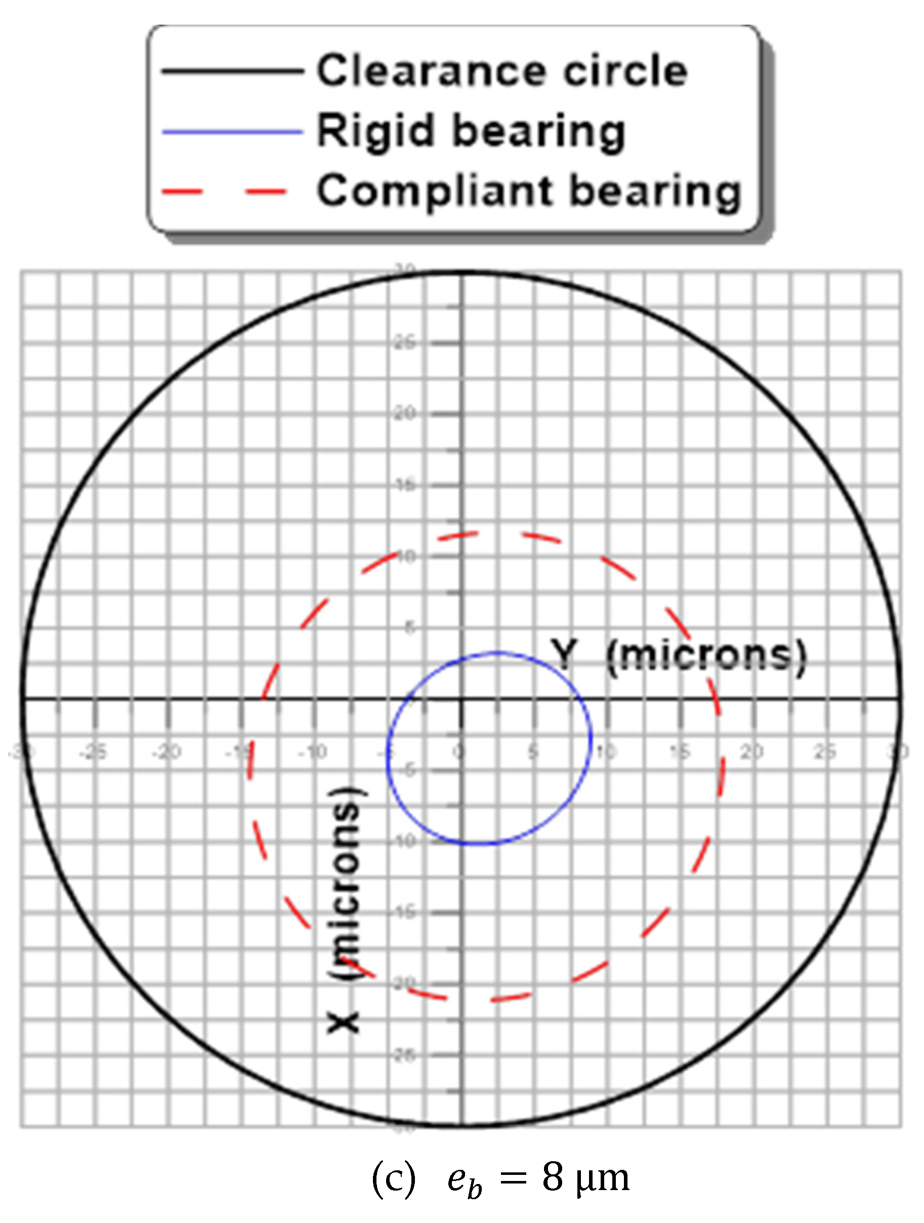
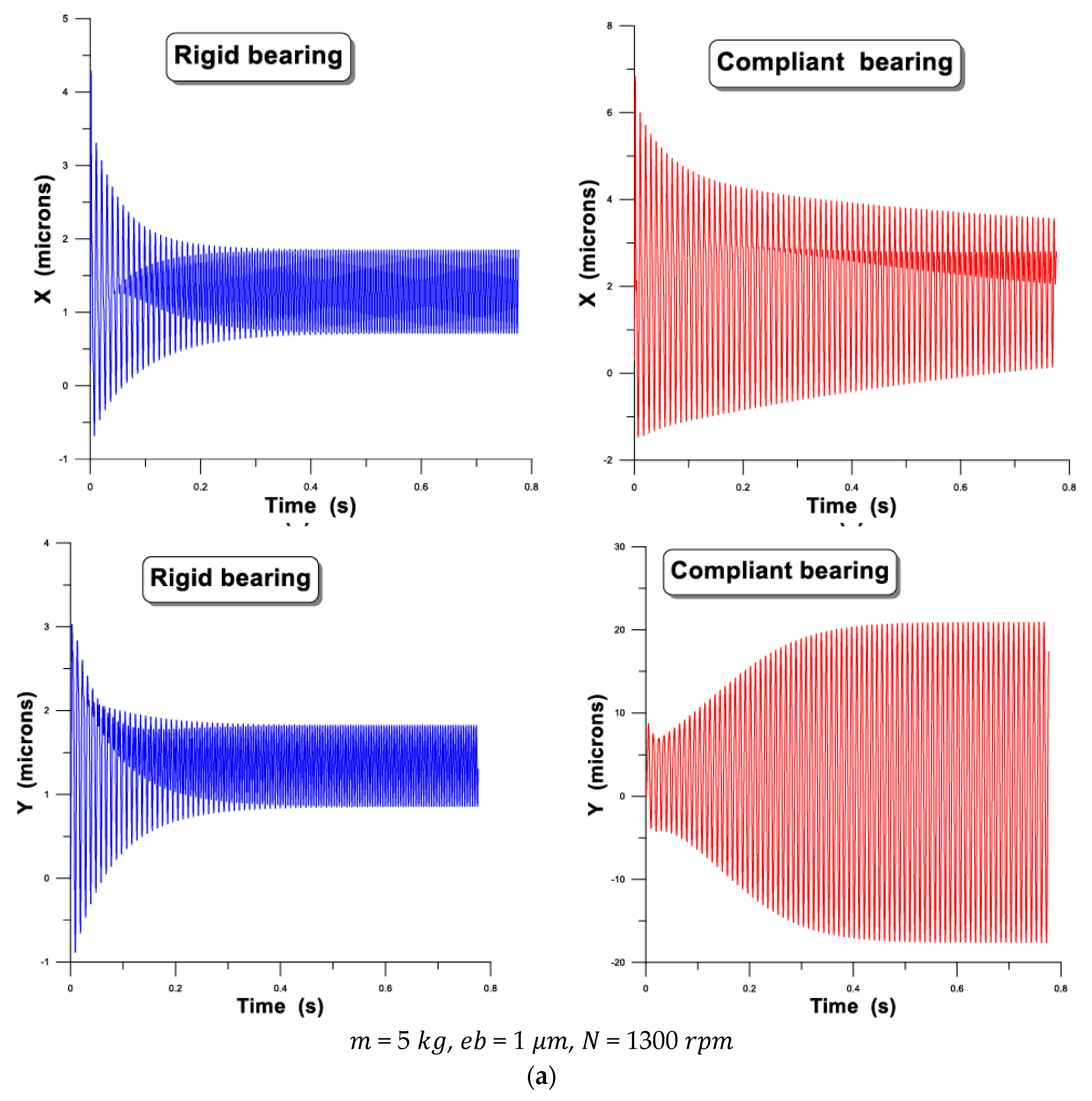
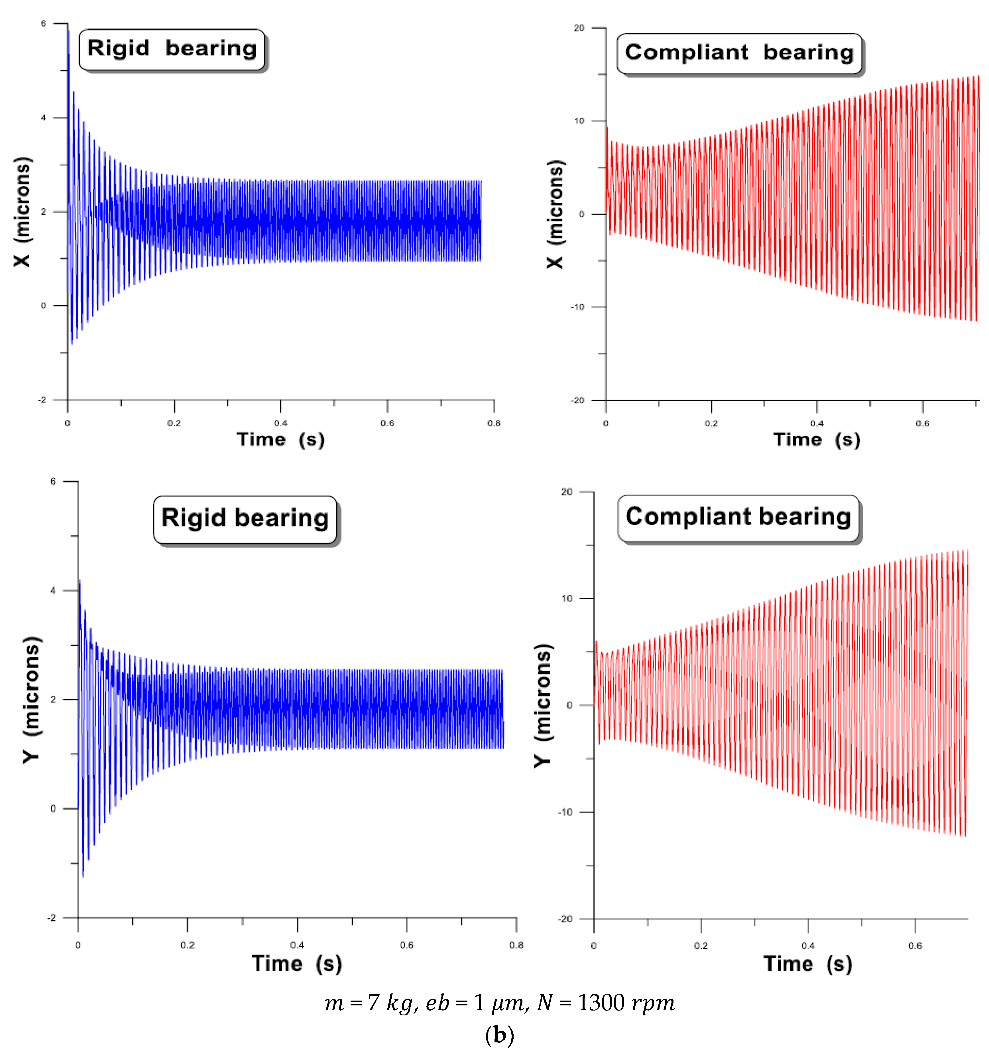
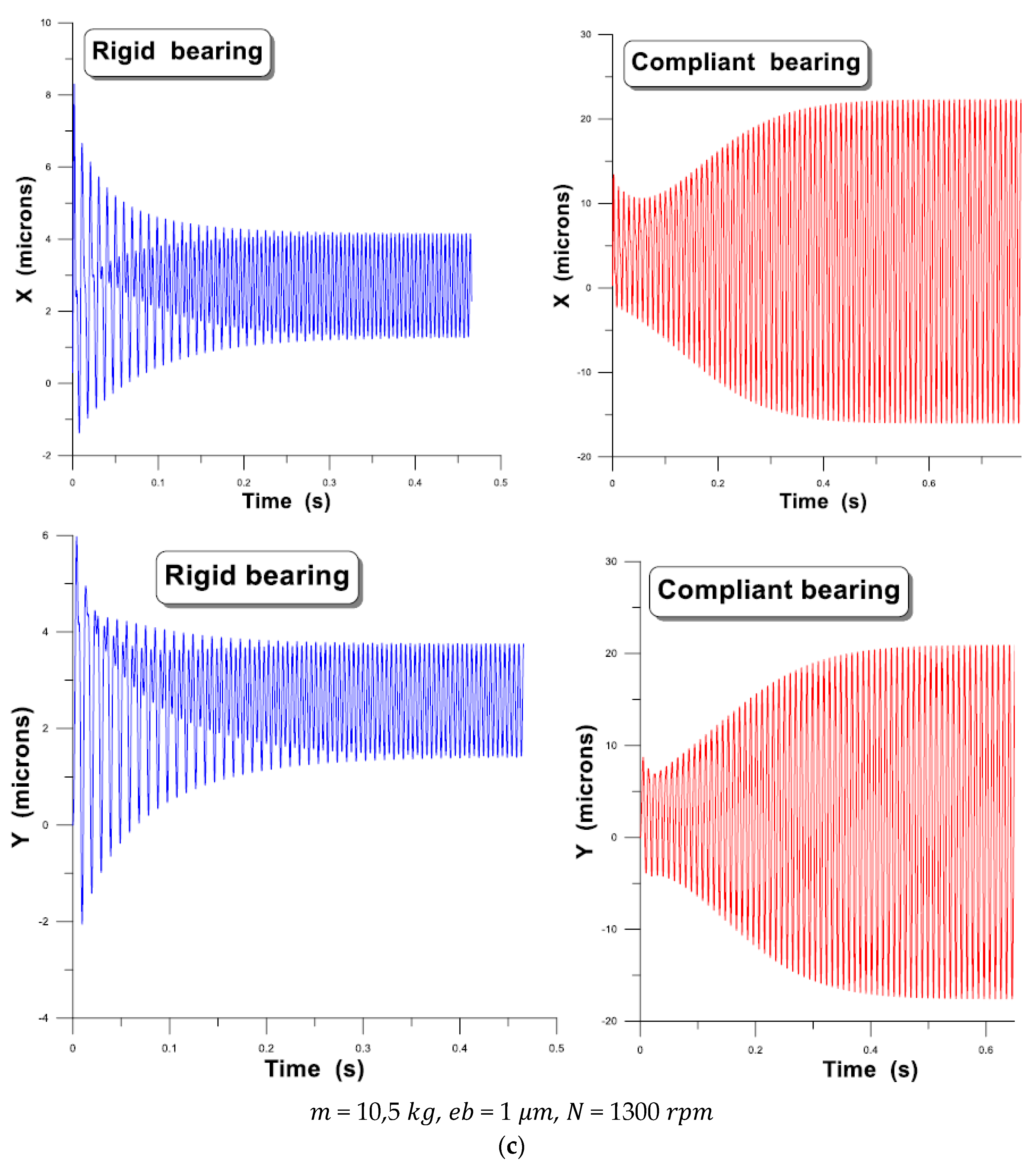
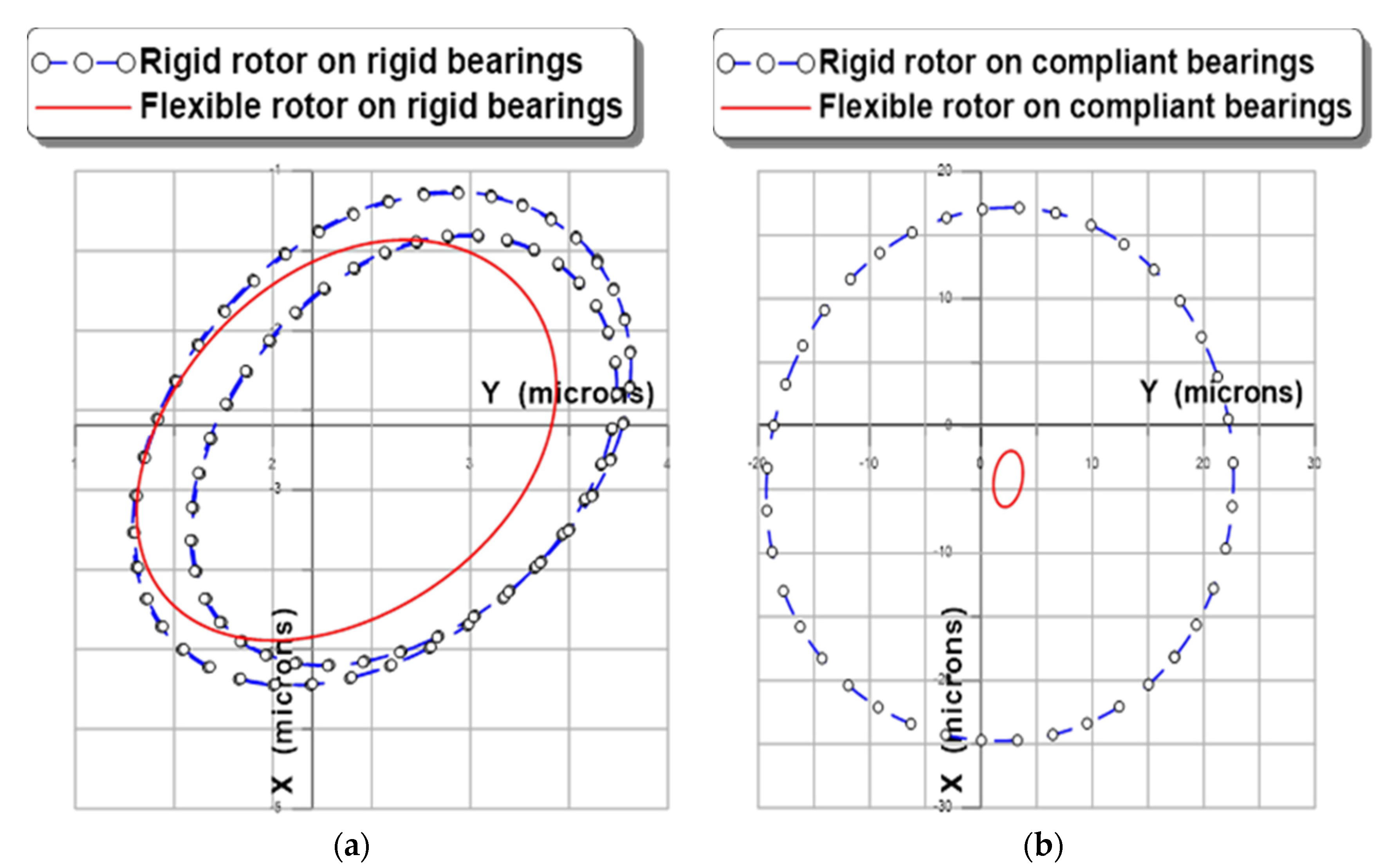
Effects of Rotor Flexibility

Figure 13 shows the centerline trajectories of the shaft calculated in the case of a rigid rotor of mass $2M$ and a flexible rotor characterized by a mass $2M$, a stiffness $2K_r$ and a damping $2C_r$ supported by two rigid aerodynamic bearings. Taking into consideration the flexibility of the rotor gives an orbit of smaller size than that calculated for a rigid rotor.

This parametric study highlights the significant effects of the elasticity of the foils and the flexibility of balanced and unbalanced rotors on the non-linear dynamic response of an aerodynamic bearing. Through these simulations, we can make the following remarks:

• The compliance of the sheets plays a negative role in the stability of the rotor-bearing system, especially for the high rotational speeds of the rotor.
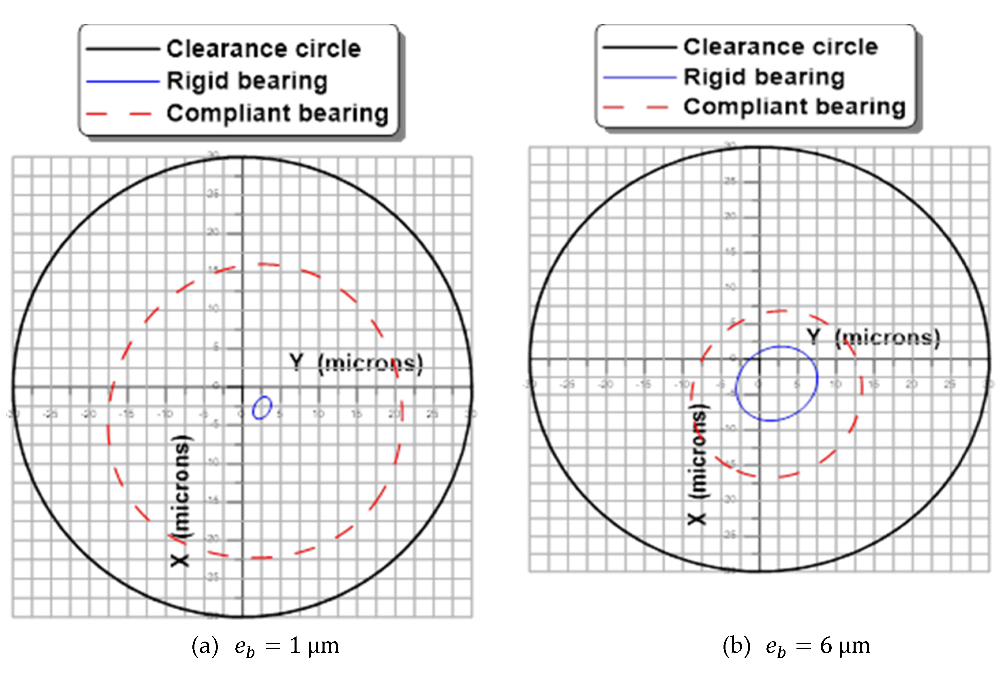
• The size of the orbit increases with the unbalance eccentricity.
• Increasing the rotor mass reduces the size of the orbit.
• The flexibility of the rotor attenuates the vibration amplitudes.

7. Conclusions

In this paper, a transient non-linear analysis was developed and presented with details to investigate the non-linear dynamic response of an unbalanced Jeffcott flexible rotor mounted in flexible foil bearing lubricated with compressible fluid. The objective was to present some results of non-linear response using a finite element method. We use a partitioned approach which treats fluid and structure as two computation domains solved separately, with their own discretization and numerical algorithm. A reason for using this approach is to reduce the development times of a monolithic code. In addition, a monolithic approach is neither easy to implement, nor to implement and evolve and difficult to manage when the geometries or the physical properties of the problem to be treated become complex. This type of method is no longer possible since each medium requires a specific approach of numerical computation procedures that the monolithic approach does not exploit. For this purpose, as a first investigation we chose to develop a simple modeling of the flexible structure. The trajectories of the shaft center were obtained numerically by solving the rotodynamic equations with Euler’s scheme. Indeed, the mathematical models do not consider the irreversible phenomena due to friction and buckling but, when comparing the rigid with compliant case, we obtain the following results:

-

Higher radial clearance;

-

Different equilibrium position;

-

Non-linear rotor trajectories;

-

Higher orbital magnitude.

In conclusion, we show the strong influence of the flexible structure on shaft trajectories. Of course, additional phenomena such as friction and 3D representation of the bump-foil structure must complete the study to give more detail [1] about the behaviors observed, but this is a first representation of the non-linear response of a flexible rotor mounted in a foil bearing.

References

1. Dykas, B.; Howard, S. Journal design considerations for turbomachine shafts supported on foil air bearings. Tribol. Trans. 2004, 47, 508–516. [Google Scholar] [CrossRef]
2. Howard, S.; Dellacorte, C.; Valco, M.; Prahl, J.; Heshmat, H. Dynamic stiffness and damping characteristics of a high-temperature air foil journal bearing. Tribol. Trans. 2001, 44, 657–663. [Google Scholar] [CrossRef]
3. Maraiy, S.Y.; Crosby, W.A.; EL-Gamal, H.A. Thermohydrodynamic analysis of airfoil bearing based on bump foil structure. Alexandria Eng. J. 2016, 55, 2473–2483. [Google Scholar] [CrossRef] [Green Version]
4. Feng, K.; Guan, H.Q.; Zhao, Z.L.; Liu, T.L. Active bump-type foil bearing with controllable mechanical preloads. Tribol. Int. 2018, 120, 187–202. [Google Scholar] [CrossRef]
5. Li, C.; Du, J.; Zhu, J.; Yao, Y. Effects of structural parameters on the load carrying capacity of the multi-leaf gas foil journal bearing based on contact mechanics. Tribol. Int. 2019, 131, 318–331. [Google Scholar] [CrossRef]
6. Tkacz, E.; Kozanecki, Z.; Kozanecka, D. Numerical methods for theoretical analysis of foil bearing dynamics. Mech. Res. Comm. 2017, 82, 9–13. [Google Scholar] [CrossRef]
7. Bonello, P.; Bin Hassan, M.F. An experimental and theoretical analysis of a foil-air bearing rotor system. J. Sound Vibration 2018, 413, 395–420. [Google Scholar] [CrossRef] [Green Version]
8. Guo, Z.; Peng, L.; Feng, K.; Liu, W. Measurement and prediction of nonlinear dynamics of a gas foil bearing supported rigid rotor system. Measurement 2018, 121, 205–217. [Google Scholar] [CrossRef]
9. Barzem, L.; Bou-Said, B.; Rocchi, J.; Grau, G. Aero-elastic bearing effects on rotor dynamics: A numerical analysis. Lubr. Sci. 2013. [Google Scholar] [CrossRef]
10. Suriano, F.J.; Dayton, R.D.; Woessner, F.G. Test Experience with Turbine-End Foil Bearing Equipped Gas Turbine Engines. In Proceedings of the ASME 1983 International Gas Turbine Conference and Exhibit, Phoenix, AZ, USA, 27–31 March 1983. [Google Scholar]
11. Heshmat, H.; Ku, C.P.R. Compliant foil bearing structural stiffness analysis: Part I—theoretical model including strip and variable bump foil geometry. ASME J. Tribol. 1992, 114, 647–657. [Google Scholar]
12. Heshmat, H.; Walowit, J.A.; Pinkus, O. Analysis of gas-lubricated foil journal bearings. J. Lubr. Tech. 1983, 105, 647–655. [Google Scholar] [CrossRef]
13. Kim, T.H.; San Andrés, L. Heavily Loaded Gas Foil Bearings: A Model Anchored to Test Data. In Proceedings of the ASME Turbo Expo 2005: Power for Land, Sea, and Air, Reno, NV, USA, 6–9 June 2005. [Google Scholar]
14. Bouchehit, B.; Bou-Saïd, B.; Garcia, M. Static and Dynamic Performances of Refrigerant-Lubricated Bearings. Tribol. Int. 2016, 96, 326–348. [Google Scholar] [CrossRef]
15. Iordanoff, I.; Bou-Saïd, B.; Meziane, A.; Berthier, Y. Effect of internal friction in the dynamic behavior of aerodynamic foil bearings. Tribol. Inter. 2008, 41, 387–395. [Google Scholar]
16. Bou-Saïd, B.; Iordanoff, I.; Grau, G. On non-linear rotor dynamic effects of aerodynamic bearings with simple flexible rotors. J. Eng. Gas Turb. Power 2007, 130, 012503. [Google Scholar] [CrossRef]
17. Carpino, M.; Talmage, G. A fully coupled element formulation for elasticity supported foil journal bearings. Tribol. Trans. 2003, 46, 560–565. [Google Scholar] [CrossRef]
18. Le Lez, S.; Arghir, M.; Frene, J. A New Bump-Type Foil Bearing Structure Analytical Model. J. Eng. Gas Turb. Power 2007, 129, 1047–1057. [Google Scholar] [CrossRef]
19. Kim, T.H.; San Andrés, L. Analysis of Gas Foil Bearings with Piecewise Linear Elastic Supports. In Proceedings of the WTC 2005, Washington, DC, USA, 12–16 September 2005. [Google Scholar]
20. Constantinescu, V. Basic relationships in turbulent lubrification and their extension to include thermal effects. J. Lubr. Tech. 1973, 95, 147–154. [Google Scholar] [CrossRef]
21. Barzem, L. Analyse théorique et experimentale de la dynamique de rotor sur paliers à feuilles lubrifié par l’air. Ph.D. Thesis, INSA Lyon, Villeurbanne, France, 2011. [Google Scholar]
22. Dhatt, G.; Touzot, J.L. Ouvrage Modélisation des structures par éléments finis; Hermès–Lavoisier–Eyrolles: Paris, France, 1992; Volume 3. [Google Scholar]
23. Zienkiewicz, O. The Finite Element Method, 3rd ed.; McGraw-Hill Book Company (UK) Limited: Maidenhead, UK, 1977. [Google Scholar]
24. Lalanne, M.; Ferraris, G.; Der Hapagopian, J. Rotordynamics Prediction in Engineering; Wiley: Hoboken, NJ, USA, 1990. [Google Scholar]
25. Zhang, J.; Kang, W.; Lin, Y. Numerical method and bifurcation analysis of Jeffcott rotor system supported in gas journal bearings. J. Comput. Nonlinear Dyn. ASME 2009, 4, 011007. [Google Scholar] [CrossRef]
26. Klit, J. Calculation of the dynamic coefficients of a journal bearing, using a variationnal approach. J. Tribol. 1996, 108, 421–425. [Google Scholar] [CrossRef]
27. Liester, T.; Seemann, W.; Bou-Saïd, B. Passive Vibration Control by Frictional Energy Dissipation in Refrigerant-Lubricated Gas Foil Bearing Rotor Systems. Proc. Appl. Math. Mech. 2018, 18. [Google Scholar] [CrossRef]
Figure 1. Garett foil bearing [10].
Lubricants 08 00014 g001
Figure 2. (a) Mohawk Innovative Technology Incorporated (MITI) foil bearing, (b) schematic of a ‘spring bearing’.
Lubricants 08 00014 g002
Figure 3. Schematic of a MITI foil bearing.
Lubricants 08 00014 g003
Figure 4. Foil bearing representation.
Lubricants 08 00014 g004
Figure 5. Schematic representation of a radial bearing with compliant bore.
Lubricants 08 00014 g005
Figure 6. Geometric details of the compliant support of a foil bearing [1].
Lubricants 08 00014 g006
Figure 7. Schematic of Jeffcott rotor supported by 2 foil bearings [25].
Lubricants 08 00014 g007
Figure 8. (ac): Shaft center trajectories for a compliant and rigid foil bearing N = 12,300   rpm and eb = 0.
Lubricants 08 00014 g008
Figure 9. Shaft center trajectories N = 30,000   rpm and eb = 0.0.
Lubricants 08 00014 g009
Figure 10. Shaft center trajectories N = 12,300   rpm and 3 values of unbalance eccentricity ratio.
Lubricants 08 00014 g010aLubricants 08 00014 g010b
Figure 11. Polar representation of shaft center trajectories N = 12,300   rpm , and eb = 1 μm and 3 values of rotor mass.
Lubricants 08 00014 g011aLubricants 08 00014 g011b
Figure 12. Cartesian representation of shaft center trajectories N = 12,300   rpm , and eb = 1 μm and 3 values of rotor mass.
Lubricants 08 00014 g012aLubricants 08 00014 g012bLubricants 08 00014 g012c
Figure 13. Comparison of shaft center trajectories for a rigid and flexible rotor ( N = 12,300   rpm , and eb = 1 μm, m = 10.5 kg, Kr = 2.03 MN/m, Cr = 103 N·s/m.
Lubricants 08 00014 g013