Abstract
Adhesive wear in dry contacts is often described using the Archard or Fleischer model. Both provide equations for the determination of a wear volume, taking the load, the sliding path and a set of material parameters into account. While the Fleischer model is based on energetic approaches, the Archard formulation uses an empirical factor—the wear coefficient—describing the intensity of wear. Today, a numerical determination of the wear coefficient is already possible and both approaches can be deduced to a local accumulation of friction energy. The aim of this work is to enhance existing energy-based wear models into the mixed lubrication regime. Therefore, the pressure distribution within the contact area will be determined numerically taking real surface topographies into account. The emerging contact area will be divided into one part of solid and a second part of elastohydrodynamically lubricated (EHL) contacts. Based on the resulting pressure and shear stress distribution, the formation of micro cracks within the loaded volume will be described. Determining a critical number of load cycles for each asperity, a locally resolved wear coefficient will be derived and the local wear depth calculated.
1. Introduction
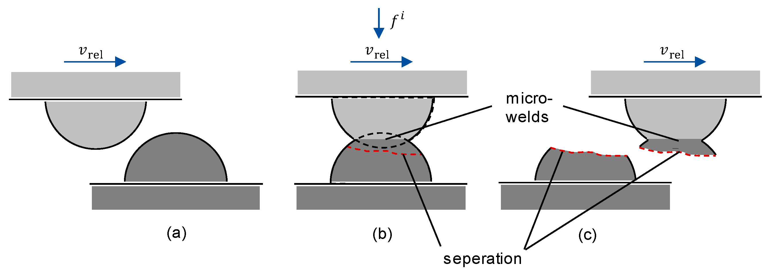
An increased application of low-viscosity lubricants in machine elements increasingly leads to operating conditions in the mixed lubrication regime along with the risk for the occurrence of wear. Since between highly loaded asperities small contact areas form, the material’s yield stress can be reached quickly and micro welds may form [1]. The subsequent separation of surfaces can occur in planes different from the original ones and material can be transferred from one body to the other. Figure 1 illustrates this process, referred to as adhesive wear, for a pair of contacting spherical shaped asperities—before (a), during (b) and after (c) the contact. The asperities are assumed to be subjected to a (local) normal load and a relative velocity .
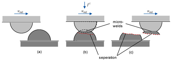
Figure 1.
Adhesive wear mechanism: (a) before contact; (b) during contact; (c) after contact [2].
Neglecting chemical effects, the occurring wear volume can be described inter alia by probabilistic models, e.g., the Archard theory [3]. Archard as well assumes spherically shaped asperities with a radius of , such that at position a circular contact area of between a pair of contacting asperities forms. He furthermore assumes this area to be so small that the occurring local pressure immediately reaches the yield stress of the surface material. According to [4], the yield stress can be equated with the surface hardness , which H leads to the relation . Since each asperity in contact is loaded by the yield stress, this relation holds for all contact spots. The volumes of evolving wear particles can each be represented by the volume of a detached asperity, which equals a hemisphere: . Defining additionally a micro sliding path in the length of the asperity diameter, , a local relative wear volume can be defined as:
By the accumulation of all local relative wear volumes for the entire contact area and considering the force equilibrium for all asperities, (where is the total normal force working on the considered system), the total relative wear volume can be given as:
The variable is the total sliding path. The factor takes into account that an instant formation of wear does not occur for every contact. It thus constitutes a parameter for the probability of the formation of wear or—in other words—for the intensity of wear. Finally, using the simplification , the total wear volume can be defined as:
Equation (3) is known as the Archard equation and the factor as the Archard wear coefficient. The wear coefficient is usually determined empirically—for metals it extends in general over a range from to [5].
Another model describing the adhesive wear mechanism was proposed by Fleischer [6]. The underlying theory is based on an energy perspective and takes the performed frictional work into account:
The factor is the friction coefficient. The intensity of wear is described by the apparent frictional energy density , which leads to the Fleischer wear equation:
Comparing Equations (3) and (5) it can trivially be derived, that the apparent frictional energy density can be given as a function of the Archard wear coefficient and vice versa:
This work focusses on the numerical determination of the Archard wear coefficient and the numerical calculation of adhesive wear in local resolution (as it was already presented in [2]). The pressure distribution, taking rough surfaces into account and being one of the main drivers for the occurrence of wear, will be calculated for both dry and mixed lubricated contacts. In the latter case, the force transmission from one body to the other through the asperity contacts is supported by an evolving pressurized elastohydrodynamic fluid film.
2. Calculation Method
2.1. Numerical Contact Model
The contact model is based on the elastic half-space theory [7] and the Hertz–Signorini–Moreau condition. The latter describes the relationship between an arbitrary gap between two surfaces within the considered area and the corresponding pressure . For dry contacts, the condition takes the following form [5]:
This condition states firstly, that an overlap of volumes cannot occur () and secondly, that in case of a mechanical contact () a pressure will evolve (). The relationship between a local pressure at position (respectively a local force ) and the resulting elastic deformation at position k can be expressed using the influence matrix , which provides the relationship between both variables [4]:
The number of asperities is . The number of elements contained in the influence matrix can quickly become very large (), especially for a finely resolved mesh. Due to the need for a high resolution (if the surface roughness shall be taken into account) this issue is tackled by means of the Method of Combined Solutions [8].
For mixed lubricated contacts, Equation (7) has to be adapted by the condition that occurring gaps will be filled with pressurized lubricant (underlying an elastohydrodynamic pressure ). The pressures within the gaps support the asperity contacts in transmitting forces form one body to the other, while at the same time separating the surfaces partwise from each other. Consequently, the number of contacting asperities decreases as well as the mechanical pressures for each contact do. According to the elastohydrodynamically lubricated (EHL) theory, a central film thickness for point contacts can be given in the following form [9]:
is a geometry parameter, a velocity parameter, a lubrication parameter and a load parameter. describes the ellipticity of the contact area. For rough surfaces, the film thickness is treated as the distance between the median planes of the deformed asperities of respective contacting surfaces. The case of mixed lubrication is defined by a fluid film, which is not sufficiently thick to separate the surfaces completely from each other. Thus, parts of the surface will remain in contact but, however, being supported by the elastohydrodynamic pressure. For contacting asperities, Equation (7) keeps being valid, while for non-contacting parts (the gaps), the formation of an elastohydrodynamic pressure is postulated. The lubricant pressure is assumed to follow the shape of the Hertzian pressure distribution for smooth surfaces [10,11] and can be given for any specific point within the contact area as:
The resulting mean value of all gaps () within the contact area equals the film thickness and thus defines the distance between a pair of contacting bodies with rough surfaces:
Satisfying Equations (7), (10) and (11), a force equilibrium between the external normal force and the sum of all solid () and EHL () forces prevails:
The number of contacting asperities is and of non-contacting asperities (gaps) . The force equilibrium and the film thickness are depicted in Figure 2.
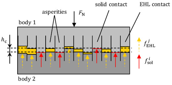
Figure 2.
Equilibrium of forces and central film thickness.
2.2. Numerical Wear Model
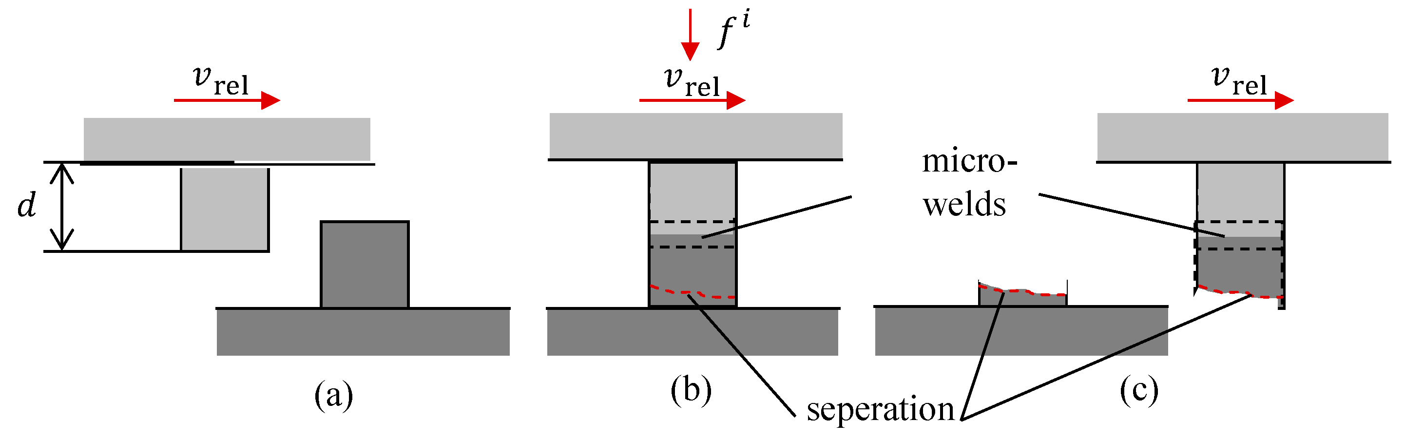
In order to develop a numerical wear model, the asperities are modelled as cubes, having an edge length of , Figure 3 (in accordance with a rectangular discretized half-space).
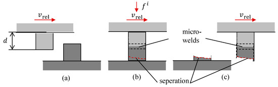
Figure 3.
Wear mechanism for cubic asperities: (a) before contact; (b) during contact; (c) after contact [2].
As described before, the wear coefficient can be understood as the probability for the detachment of a single wear particle. It thus forms the reciprocal value of a number of sustainable load cycles and can be written as [3,12]:
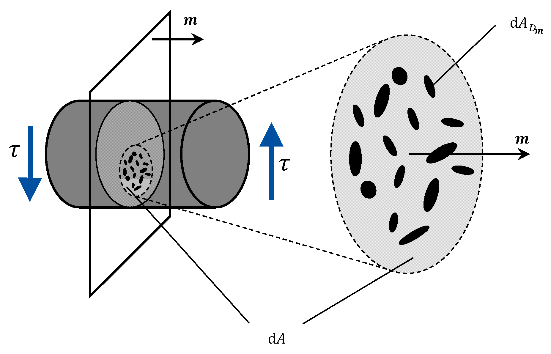
For a numerical calculation of , the theory of Continuum Damage Mechanics is used, describing the progressive weakening of solid materials under a cyclic shear stress [13,14,15,16]. In Figure 4 a control volume, loaded by a cyclic shear stress is shown. The damaged area consists of several micro cracks, depicted as black areas (), while the control area is represented in light gray.

Figure 4.
Micro cracks and weakened cross section [2,17].
It is assumed that any load above a specific endurance limit will cause micro cracks within the loaded volume. The ratio of the damaged area , defined by the normal vector , to a cross section can be expressed as [17]:
The factor is a probability factor. For isotropic materials, the damage ratio is independent of the normal direction , which leads to . The damage propagation increases exponentially and can be expressed as a function of the performed load cycles [17]. If the endurance limit is not reached, no damage propagation will occur:
The parameter describes the amount of damage propagation and can be given as follows [18]:
The parameter is the hardening coefficient, the hardening exponent and the true failure stress [18]. If after cycles a critical value is reached, the number of load cycles performed equals the critical number: .
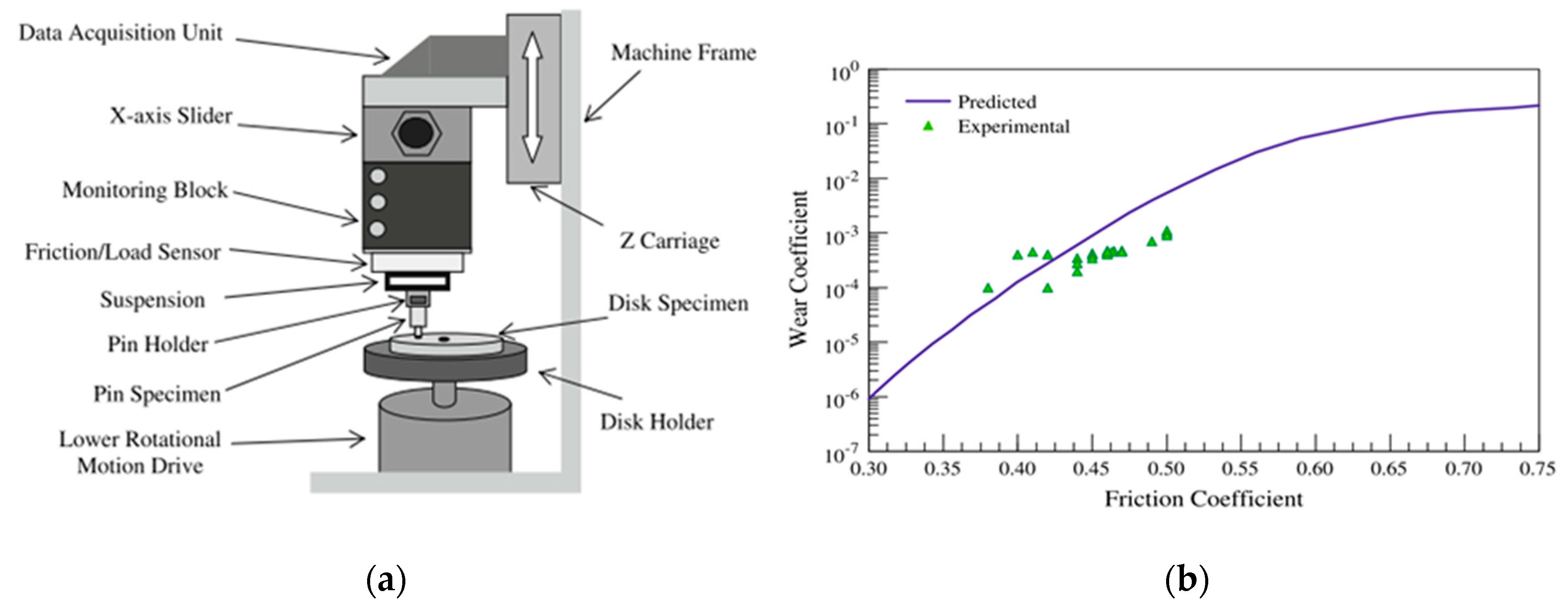
The validity of the model was proved by Beheshti et al. in [18] by a comparison of predicted wear coefficients and experimental results as a function of the friction coefficient. In Figure 5, the comparison for aluminum 6061-T6 is depicted, while the experiments where conducted on a pin-on-disk test. The tests were conducted with a pin (diameter 8 mm) made of aluminum in contact with a disk made of stainless steel (SS 304, diameter 100 mm). The sliding velocity was set within a range of , the normal load in a range from . The test duration was . The amount of wear was obtained by weighing the pin before and after the test.
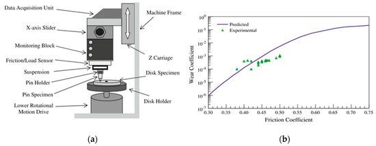
Figure 5.
Pin-on-disk tribometer (a) and comparison of experimental and simulation results (b) for the prediction of the wear coefficient [18].
Applying the aforementioned model to all contacting asperities, the wear coefficient can be determined in local resolution. Therefore it is assumed, that the asperity is loaded by a cyclic shear stress , which is the product of the local pressure and the friction coefficient:
Thus, the local wear coefficient is instantly a function of the local shear stress. Assuming an incremental wear path in the length of (element edge length) and an incremental wear volume of (volume of a cubic element), the local relative wear volume now takes the form:
Here, the probability (or wear-) coefficient is considered in local resolution. Rearranging the equation and using the relationship , the local wear depth can be expressed as . Taking additionally the number of load cycles into account, the cumulative wear path can be considered. The locally resolved wear depth can finally be given in the form of a vector:
2.3. Calculation Algortihm
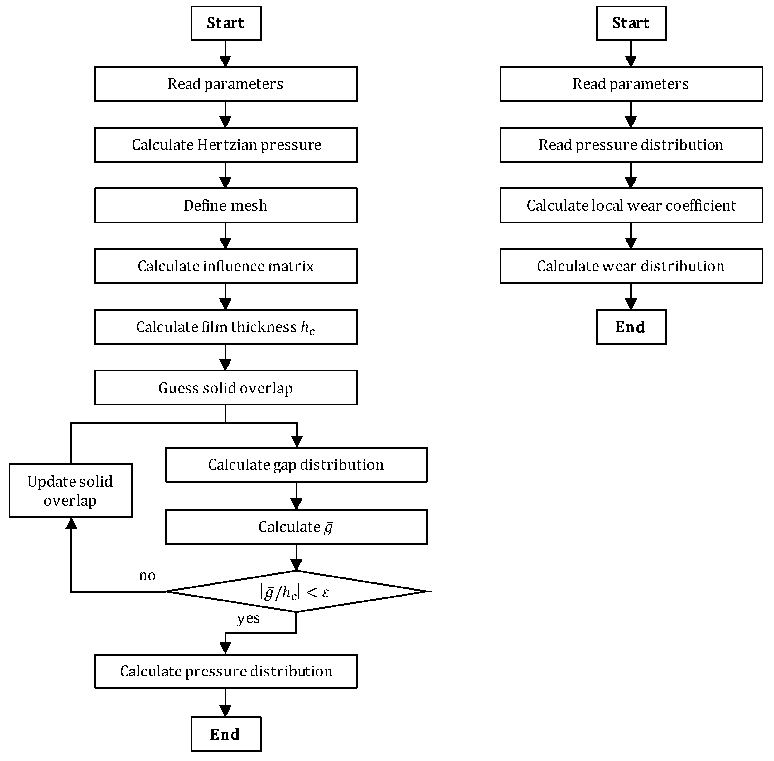
The simulation follows the algorithm depicted in Figure 6. The left side shows the calculation of the pressure distribution, which follows an iterative approach. The first step is to read the material, geometry and load parameters. Based on this, the Hertzian pressure distribution is calculated and the discretized mesh is defined. For the determination of the pressure distribution the influence matrix is calculated. Depending on the fluid and the EHL parameters, a film thickness is calculated. Before the calculation starts, an initial guess of the solid body overlap is estimated and imprinted on the system. Taking the micro geometry and the solid body overlap into account, the gap distribution is calculated based on the elasto-plastic half space. Within the Hertzian contact area a mean value of the gap distribution is determined. If the deviation between and the film thickness exceeds a specific limit , the solid overlap is updated (increased in case of and decreased in case of ) and the calculation will be repeated. If the deviation is small enough, the mean gap is assumed to be equal the EHL film thickness and the iteration is finished. Finally, the calculation of the solid pressure distribution follows, the local wear coefficient is calculated and the wear distribution is determined (right side of Figure 6).

Figure 6.
Simulation algorithm. (Left): Simulation of pressure. (Right): Simulation of wear.
3. Simulation Results
3.1. Model System
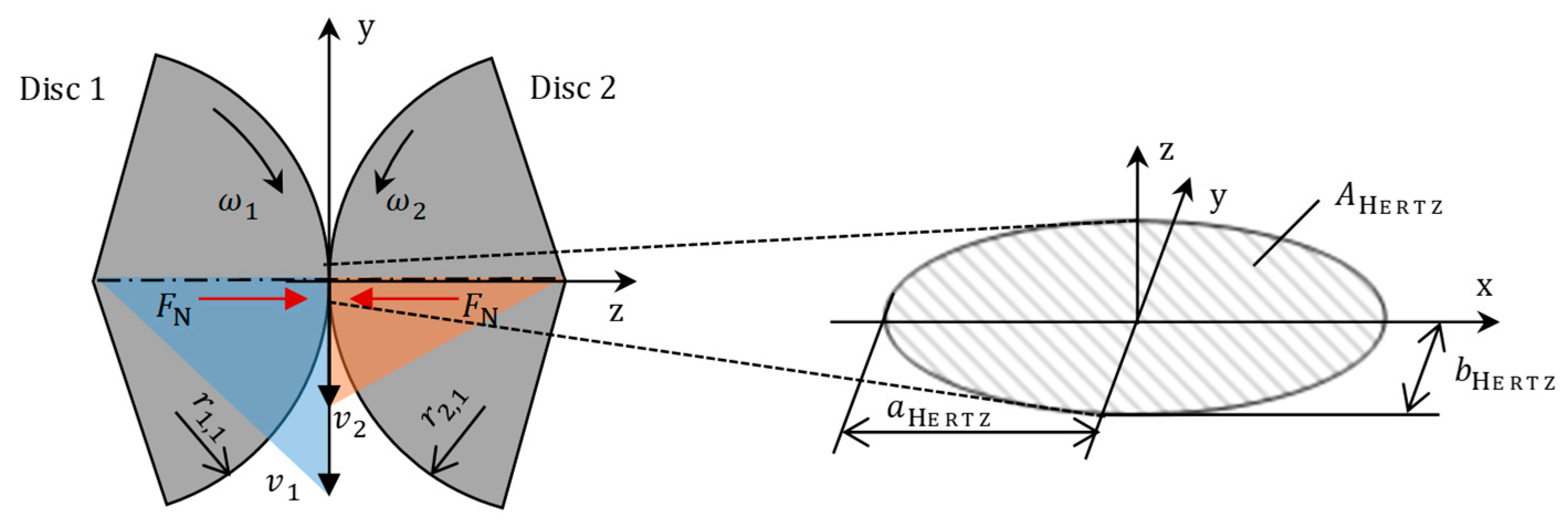
Although the presented contact and wear models have been developed to describe wear in machine elements like bearings or gears, for investigations into the wear mechanism it is more suitable to abstract the geometry to a simplified model system. Thus, characteristic contact geometries and loading situations of rolling element bearings have been transferred to a model contact consisting of two discs. The material is bearing steel 100Cr6 (AISI52100). The discs are pressed together by a normal force of . Each disc has a radius of and is driven independently from the other with different circumferential velocities ( and ). Thus, in the contact area an entrainment velocity of and a relative velocity of evolve, depicted in Figure 7.

Figure 7.
Model system.
Disc 1 is additionally equipped with a crowning radius of The contact and load parameters lead to a Hertzian pressure of . The root mean squared (RMS) roughness of the discs is . The dynamic viscosity of the lubricant is . The entrainment velocity is responsible for the formation of an EHL film, which takes a value of , respectively a specific film thickness of . The contact area is discretized into square elements with an edge length of . According to the half-space theory, the surface geometries of both discs are projected to one resulting (combined) model surface, which contacts to an opposing flat elasto-plastic half-space surface. In Table 1 the material, geometry and simulation parameters are listed.

Table 1.
Material, geometry and simulation parameters [18,19].
3.2. Simulation of Gap and Pressure Distributions
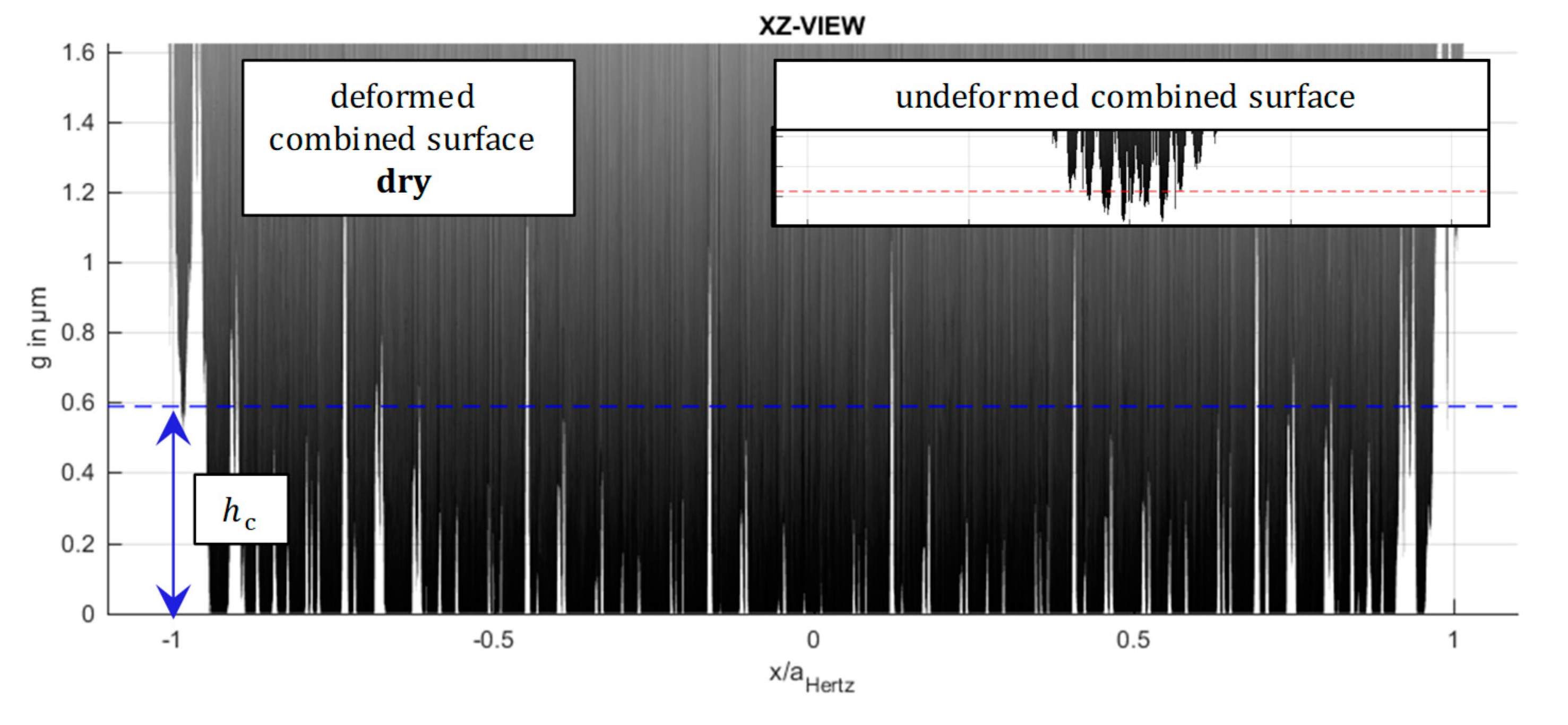
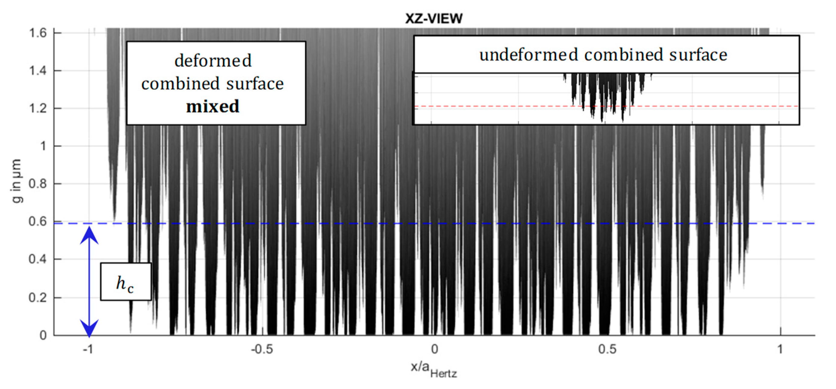
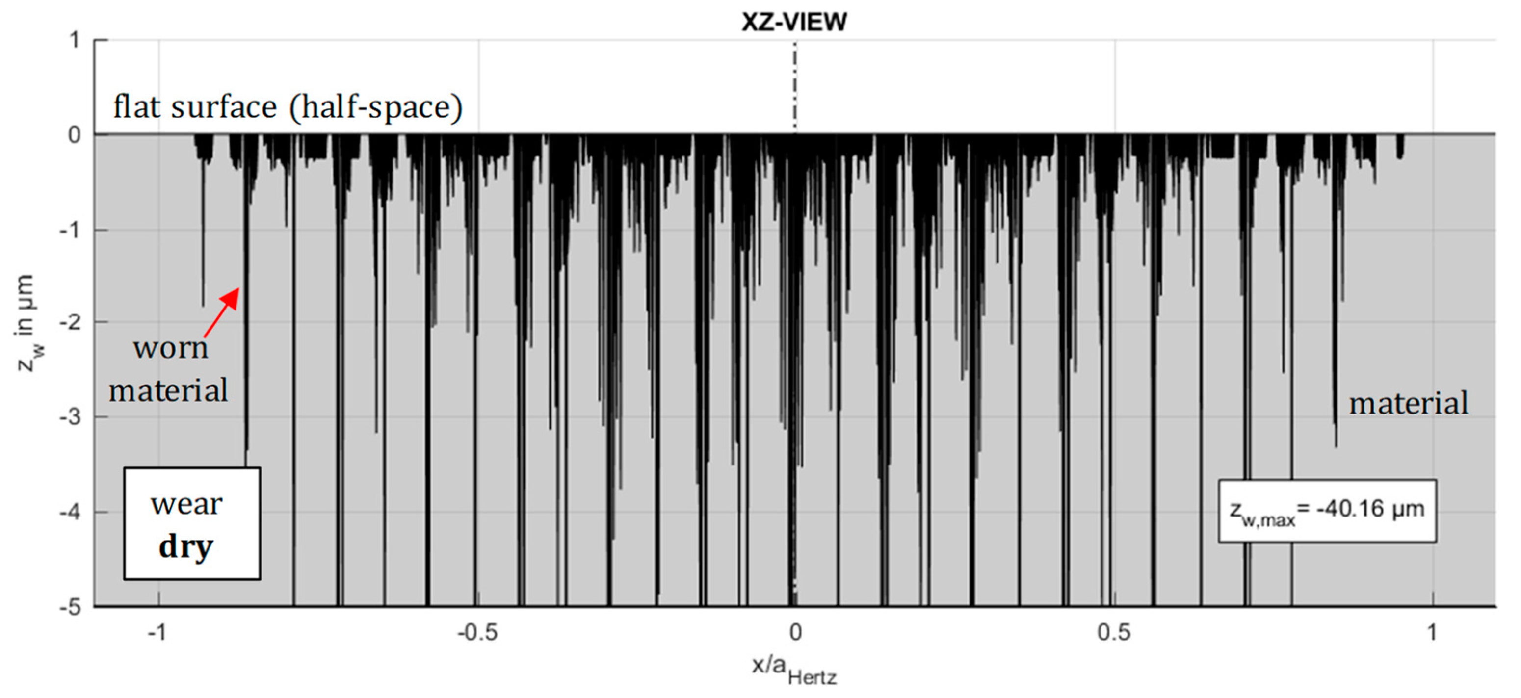
The results of the simulation of the gap distribution for a dry and a mixed lubricated contact are depicted in the following Figure 8 and Figure 9. In Figure 8 the side view (XZ view) of the deformed surface geometry between the combined surface (black) and the half-space surface (zero line) for a dry contact is shown. The gap height (in -direction) is given in on the ordinate, while the abscissa shows the -direction along the long half-axis. The latter is normalized to the Hertzian contact length . On the top right corner, the corresponding undeformed surface is depicted keeping the aspect ratio constant. The numerically calculated film thickness is (for mixed lubrication), which is marked by a blue dotted horizontal line. Because of numerical deviations the calculated film thickness differs slightly from the analytical solution of .
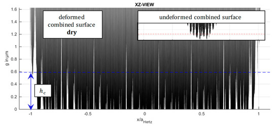
Figure 8.
Gap distribution for dry contact (XZ view).

Figure 9.
Gap distribution for a mixed lubricated contact (XZ view).
Figure 9 shows the corresponding results for mixed lubrication. It can be seen, that due to the supporting effects of the EHL pressure the deformation and the number of contacting asperities has significantly decreased.
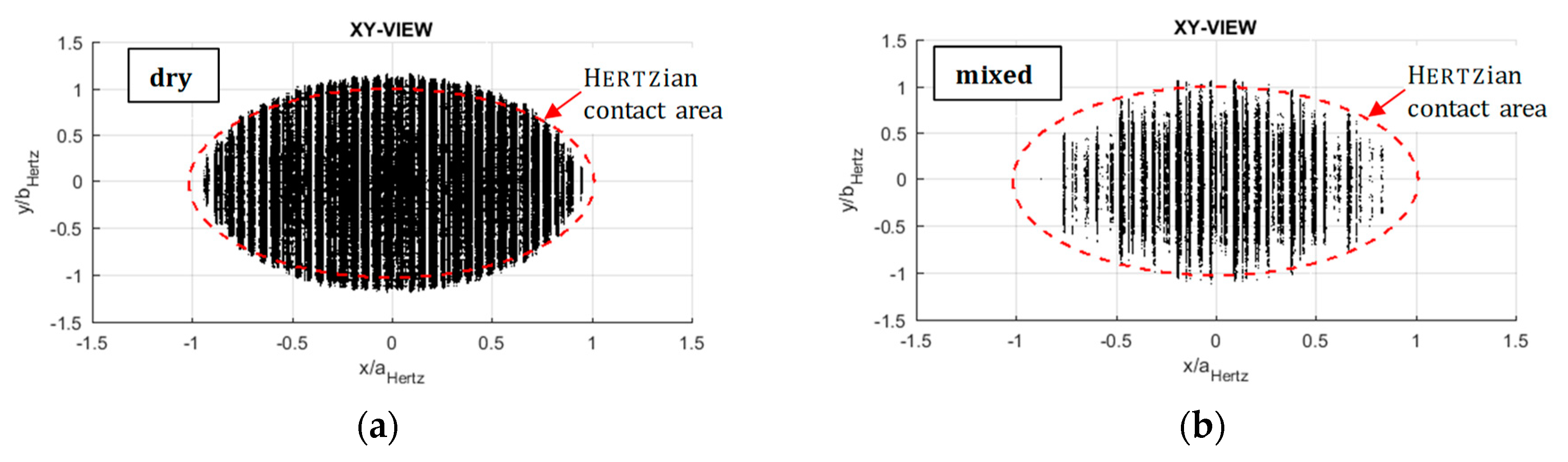
In the following Figure 10, Figure 11 and Figure 12 the simulation results for the pressure distribution are depicted. In each figure, the results for a dry contact are shown on the left side, results for mixed lubrication on the right. In both cases, only the occurring pressures for contacting asperities are drawn, meaning that the EHL pressures are blanked out. Figure 10 shows the top (XY) view of the contact zone. The abscissa again shows the -direction along the long half-axis () of the contact zone, while the ordinate shows the -direction along the short half-axis (). Both axes are normalized to the respective Hertzian contact length. It can be seen, that the dry contact fills out almost the entire Hertzian contact area (denoted in red dotted line), while the mixed contact area does not. Furthermore, a cyclic waviness can be identified, which corresponds to a waviness of the surface along the -direction due to the manufacturing process.

Figure 10.
Pressure simulation results—XY view. (a) Dry contact. (b) Mixed lubricated contact.
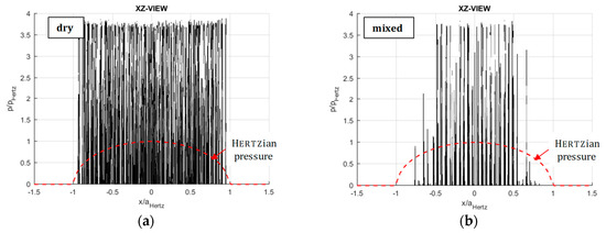
Figure 11.
Pressure simulation results—XZ view. (a) Dry contact. (b) Mixed lubricated contact.
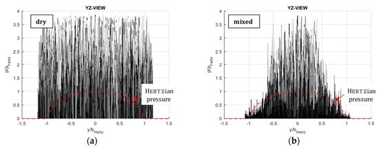
Figure 12.
Pressure simulation results—YZ view. (a) Dry contact. (b) Mixed lubricated contact.
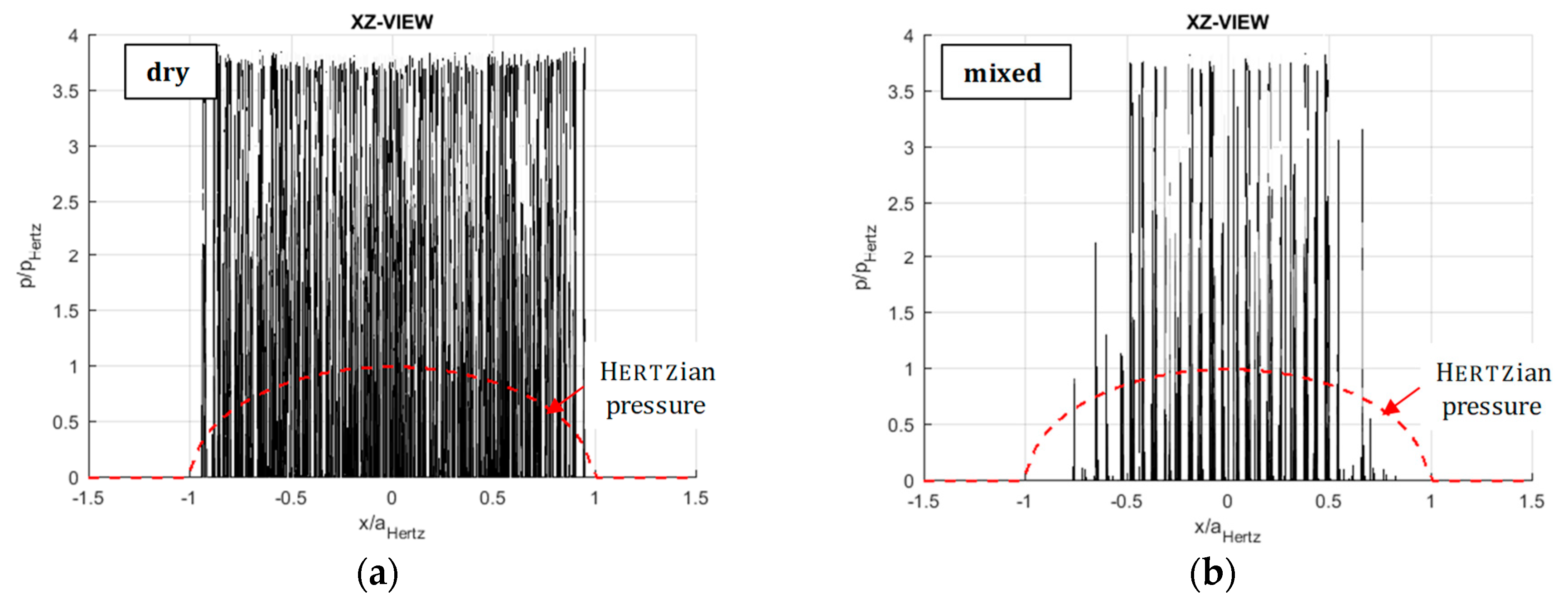
For the case of a dry contact, the sum of all local forces leads to , an EHL part does not exist (see Equation (12)):
Slight deviations from the input values occur due to numerical approximations.
For the mixed lubricated contact, the sum of all local solid forces is:
Thus, the percentage of the force, transmitted through asperity contacts is much lower, than in the case of a dry contact: . The remaining part of the total force, , has to be transmitted by the lubricant film:
In Figure 11 the pressure distribution is shown in the XZ view. The abscissa now shows the long half-axis () and the ordinate shows the normalized pressure . The red dotted line depicts the corresponding Hertzian pressure distribution for smooth surfaces. In both cases (dry and mixed), a multitude of asperities reaches the yield stress, why the maximum achievable normalized pressure is limited to . The pressure density is much higher in the case of the dry contact, as it also can be observed in Figure 10.
Finally, Figure 12 shows the pressure distribution in YZ view. The abscissa now shows the short half-axis ().
3.3. Simulation of Wear Distribution
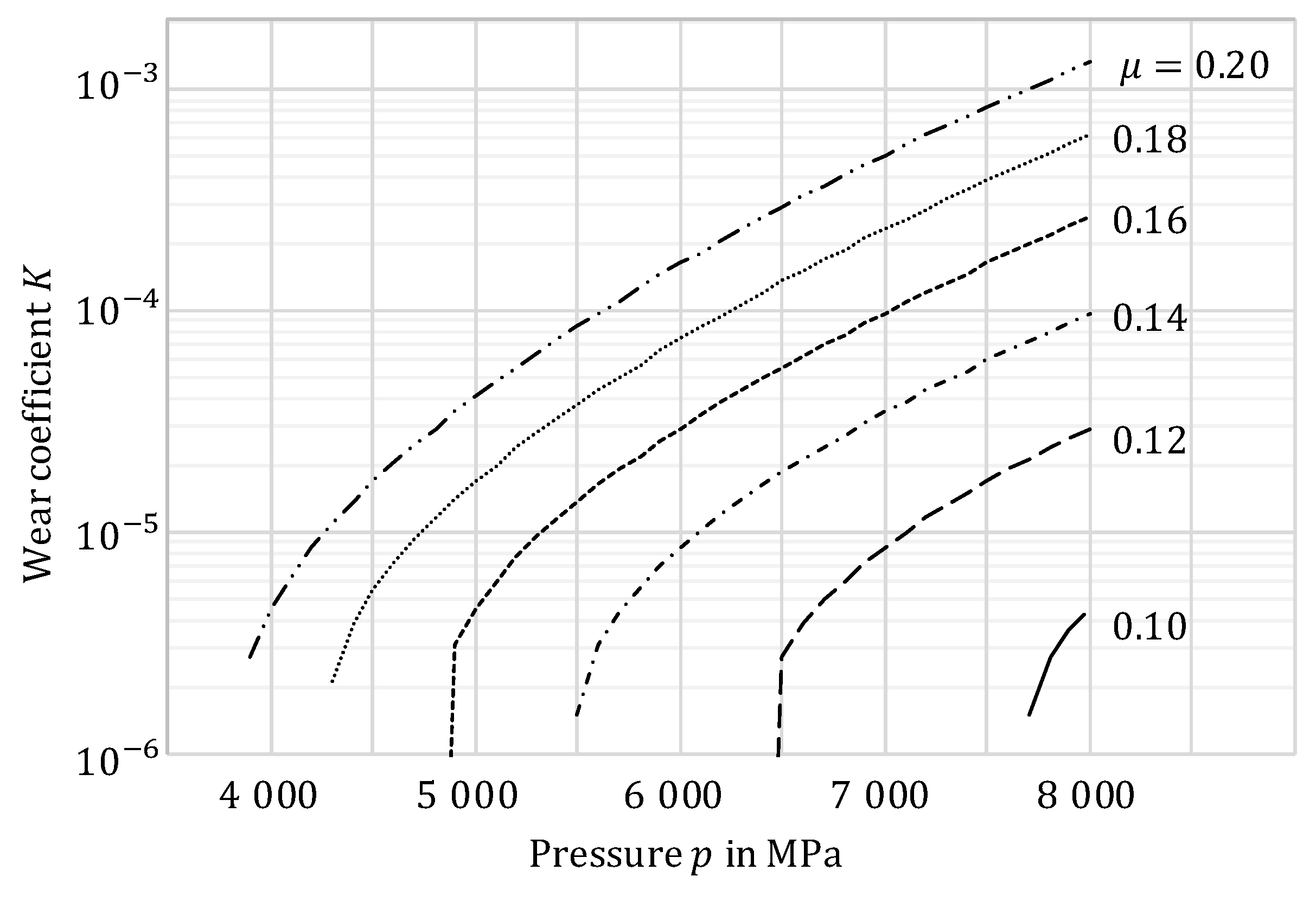
The simulation of the adhesive wear follows the model presented in Section 2.2 and Section 2.3. The shear stress and thus the friction coefficient and local pressure have large impacts on adhesive wear. While the local pressure can be calculated numerically as shown in the previous chapter, the determination of the (solid) friction coefficient is still difficult. To illustrate the influence of both parameters on the wear coefficient, a parameter study was carried out. Varying the (local) pressure in a range of 3500 to 8000 MPa and the friction coefficient in a range of to leads to wear coefficients of up to (while the minimum value for the wear coefficient was set to , according to [5]). In Figure 13 the corresponding curves are depicted.

Figure 13.
Wear coefficient as a function of the friction coefficient and the (local) pressure.
Within this work a friction coefficient of is assumed such that the calculated wear coefficient lies within an interval of . The simulated test duration is . While the mean values of all local wear coefficients do not differ significantly for the dry and the mixed lubricated case (, ), the number of asperities in contacts does: , . In order to derive a characteristic parameter, describing the intensity of wear for each considered system, the mean value can be multiplied by the respective number of contacting asperities:
The factor shall here be referred to as the wear intensity factor. The ratio between both, the mixed lubricated and the dry factor, is and thus of a similar magnitude to the percentage of force, transmitted through asperity contacts ().
Figure 14 depicts the simulation results for the wear depth (according to Equation (19)) for the dry contact. It shows a section through the XZ plane, while the total wear volume is distributed evenly over the entire circumference of the discs. The wear depth (depicted in black color) for both contacting bodies is projected to the half-space, depicted in gray color. The abscissa is showing the -direction along the long half-axis () of the contact zone, while the ordinate shows the wear depth. It can be seen, that the occurring wear spreads over the entire contact zone, although areas of high work density (i.e., high product of relative velocity and pressure) show a significantly higher density of wear (here: in the central area, where the amount of pressure is the largest). The maximum peaks reach values of , which are not shown within the scale due to a better resolution of the figure.

Figure 14.
Wear simulation results for a dry contact (XZ section).
In Figure 15 the corresponding wear for the mixed lubricated contact is shown. It is trivial, that a reduction of solid forces due to the formation of a supporting fluid film leads to a reduction of wear. As already shown, the wear intensity factor is significantly lower in case of the mixed regime. The occurring wear decreases in general, while the maximum wear in particular decreases to a value of .
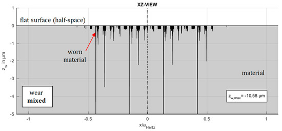
Figure 15.
Wear simulation results for a mixed lubricated contact (XZ section).
4. Conclusions and Outlook
Within the presented work, simulation results for a dry and a mixed lubricated contact have been shown and compared. The wear depth has been determined by calculating a pressure distribution, taking a rough surface geometry into account, and subsequently calculating a locally resolved and energy-based wear coefficient. It has been shown that the cumulative force, transmitted by contacting asperities can be reduced by an evolving elastohydrodynamic film, followed by a significant reduction of wear. The results show a high accumulation of wear for specific spots of single sharp asperities, while it is assumed not to correspond to real systems. It should be noted, that it is possible to avoid this numerical fault by updating the contact geometry after each load cycle, such that the pressure distribution will adapt the new geometry and the high pressure regime will relocate to less-worn areas. The disadvantage of this approach is the strongly increasing computing time. The calculation of the pressure distribution takes by far the majority of the entire calculation time. In addition, the creation of wear-resistant chemical layers, built up by chemical additives, may be taken into account in future works.
Besides the pressure, the coefficient of friction is the main driver for the amount of the calculated wear coefficients. In this work, the coefficient of friction is assumed to be 0.12, which involves huge uncertainty. Further work is therefore focused on the numerical and experimental determination of the friction coefficient.
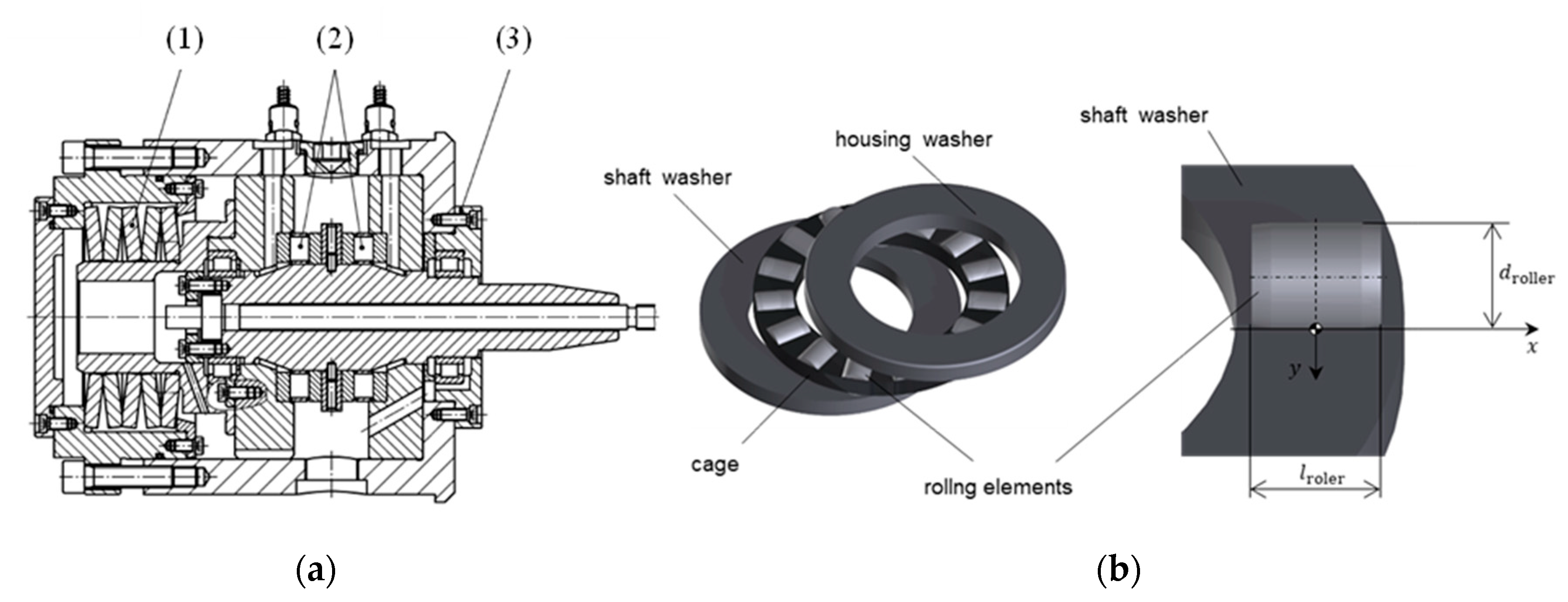
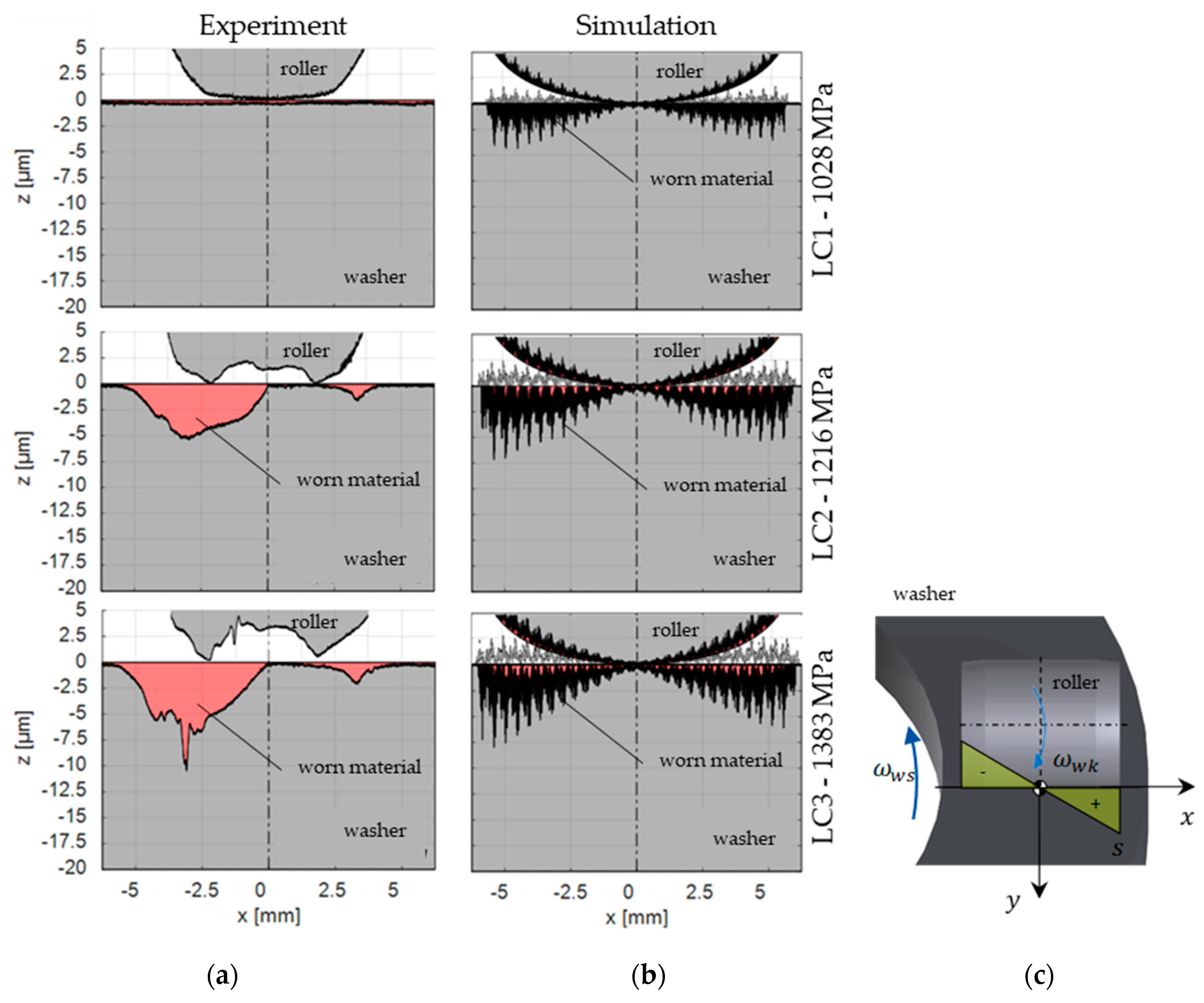
Furthermore, an experimental validation of the wear model on real machine elements will be the subject of future works. As already shown in [2], wear in machine elements shows several effects, which are not considered in this paper. Nevertheless, experiments were already carried out on thrust roller bearings in [2] and show a basic agreement of experimental and simulation results. The experimental part was conducted using an FE8 test rig [20], Figure 16.

Figure 16.
FE8 test rig (a) [20] and test bearing (b).
In this test rig, two test bearings (2) are mounted on a common shaft, while the housing washers are fixed in the housing. The shaft is radially supported by two cylindrical roller bearings and driven by an electric motor. A static axial load is applied through a cup spring assembly (1) such that both test bearings are subjected to the same load. The test lubricant was a mineral oil (viscosity at ). The investigations were carried out at low relative speeds between the contacting bodies, so that the film thickness ratio was also low (). Three load cases with axial loads of , and were defined, resulting in Hertzian pressures of , and , respectively. For each load case (LC) a test with a constant shaft speed of was conducted. Each test duration was ( shaft revolutions). The resulting experimental wear volume was determined by tactile measurement of the profile before and after each test. The corresponding simulations were conducted without consideration of an EHL film and assuming a friction coefficient of .
In Figure 17 the results of the experiments are shown on the left side (a) and for the simulations in the middle (b). The left half of each picture is the inner part of the washer/roller contact. In this region negative slip occurs, while on the outer part (right half) positive slip occurs. In load case 1, little to no wear can be observed. In load case 2, a wear depth of around in the area of the negative slip occurred, while in the area of positive slip considerably less wear can be observed. In load case 3, the wear depth is around . The simulation results show that the amount of wear can be calculated in the right order of magnitude, but the correct prediction of the local amounts is still difficult. Two of the reasons may be the missing consideration of additional wear mechanisms, like abrasive wear, and the missing consideration of the influence of positive/negative slip.
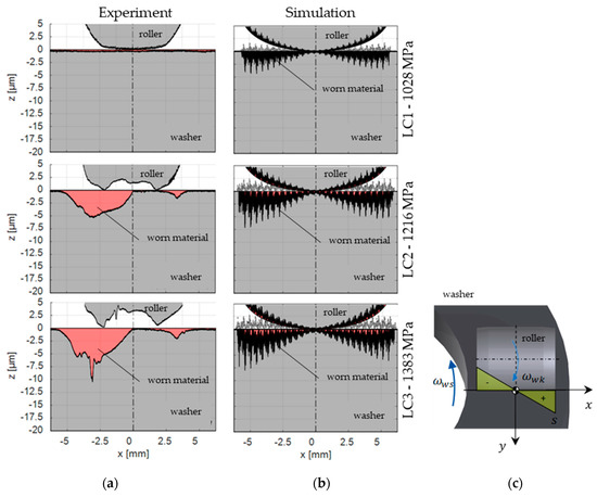
Figure 17.
Experimental (a) and simulation results (b), FE8 test rig [2]. Kinematics in test bearings (c).
Author Contributions
Conceptualization, J.T.T. and G.P.; methodology, J.T.T. and G.P.; software, J.T.T. and M.A.F.; validation, J.T.T. and M.A.F.; formal analysis, J.T.T. and M.A.F.; investigation, J.T.T. and M.A.F.; resources, G.P. and F.P.; data curation, M.A.F.; writing—original draft preparation, J.T.T.; writing—review and editing, M.A.D., F.P. and G.P.; visualization, J.T.T. and M.A.F.; supervision, G.P.; project administration, J.T.T. and F.P.; funding acquisition, J.T.T., F.P. and G.P. All authors have read and agreed to the published version of the manuscript.
Funding
The publication of this article was funded by the Open Access Fund of the Leibniz University Hannover, Germany.
Conflicts of Interest
The authors declare no conflict of interest.
List of Symbols
| Micro contact area at pos. | Archard Wear coefficient at pos. | ||
| Hertzian contact length | Normalized pressure | ||
| Parameter (film thickness) | Normalized flow pressure | ||
| Damage propagation after load cycles | Pressure | ||
| Hertzian contact width | Pressure at pos. | ||
| Influence matrix | Hertzian pressure | ||
| Damage variable | Pressure acc. to Hertz at pos. | ||
| Critical damage | Flow pressure | ||
| Damage variable after load cycles | Solid pressure at pos. | ||
| Element length | Geometry parameter | ||
| Cross section | RMS roughness | ||
| Young’s modulus | Asperity radius | ||
| App. frict. energy density | , | Radius disc 1, plane 1/2 | |
| Normal force at pos. | Radius disc 2, plane 1/2 | ||
| Solid force at pos. | Sliding path | ||
| EHL force at pos. | Sliding path vector | ||
| Normal force | Micro sliding path at pos. | ||
| Solid force | Duration | ||
| Solid force, dry contact | Velocity parameter | ||
| Solid force, mixed contact | Wear volume | ||
| EHL force | Micro wear volume at pos. | ||
| EHL force, dry contact | Entrainment velocity | ||
| EHL force, mixed contact | Circumferential velocity body 1 | ||
| Lubrication parameter | Circumferential velocity body 2 | ||
| Gap | Relative velocity | ||
| Gap at pos. | Deformation at pos. | ||
| Mean gap | W | Load parameter | |
| Surface hardness | Frictional work | ||
| Film thickness | Z | Number of asperities | |
| Wear intensity factor | Wear depth at pos. | ||
| Position | Wear depth vector | ||
| Hardening coefficient | Dynamic viscosity | ||
| Hardening exponent, | Specific film thickness | ||
| Number of elements in -direction | Ellipticity | ||
| Normal vector | Friction coefficient | ||
| N | Number of elements in -direction | ν | Poisson’s ratio |
| Critical number of load cycles | Shear stress | ||
| , | Number of load cycles | Endurance limit | |
| Number of non-contacting asperities | True failure stress | ||
| Number of contacting asperities | Shear stress at pos. | ||
| Archard Wear coefficient | Damaged area | ||
| Archard Wear coefficient vector | |||
| K1, k | Probability factor |
References
- Bowden, F.P.; Tabor, D. The Friction and Lubrication of Solids, 2nd ed.; Clarendon Press: Oxford, UK, 1954. [Google Scholar]
- Terwey, J.T.; Berninger, S.; Burghardt, G.; Jacobs, G.; Poll, G. Numerical Calculation of Local Adhesive Wear in Machine Elements under Boundary Lubrication Considering the Surface Roughness. In Proceedings of the 7th International Conference on Fracture Fatigue and Wear. (FFW 2018), Ghent, Belgium, 9–10 July 2018. [Google Scholar]
- Archard, J.F. Contact and Rubbing of Flat Surfaces. J. Appl. Phys. 1953, 24, 981–988. [Google Scholar] [CrossRef]
- Bartel, D. Berechnung von Festkörper-und Mischreibung bei Metallpaarungen; Shaker: Aachen, Germany, 2001. [Google Scholar]
- Wriggers, P. Computational Contact Mechanics, 2nd ed.; Springer: Berlin, Germany, 2006. [Google Scholar]
- Fleischer, G.; Gröger, H.; Thum, H. Verschleiß und Zuverlässigkeit; VEB Verlag Technik: Berlin, Germany, 1980. [Google Scholar]
- Love, A.E.H. The Stress Produced in a Semi-Infinite Solid by Pressure on Part of the Boundary. Philos. Trans. R. Soc. 1929, 228, 377–420. [Google Scholar]
- Brecher, C.; Renkens, D.; Löpenhaus, C. Method for Calculating Normal Pressure Distribution of High Resolution and Large Contact Area. J. Tribol. 2016, 138. [Google Scholar] [CrossRef]
- Hamrock, B.J.; Dowson, D. Ball Bearing Lubrication—The Elastohydrodynamics of Elliptical Contacts; John Wiley & Sons: New York, NY, USA, 1981. [Google Scholar]
- Hertz, H. Ueber die Berührung fester elastischer Körper. J. Reine Angew. Math. 1881, 92, 156–171. [Google Scholar]
- Harris, T.A.; Kotzalas, M.N. Rolling Bearing Analysis—Essential Concepts of Bearing Technology, 5th ed.; CRC Press: Boca Raton, FL, USA, 2007. [Google Scholar]
- Archard, J.F. Wear Theory and Mechanisms. In Wear Control Handbook; Peterson, M.B., Winer, W.O., Eds.; American Society of Mechanical Engineers: New York, NY, USA, 1980; pp. 35–80. [Google Scholar]
- Bhattcharya, B.; Ellingwood, B. A Damage Mechanics Based Approach to Structural Detoriation and Reliability; Oak Ridge National Laboratory: Baltimore, MD, USA, 1998. [Google Scholar]
- Bhattcharya, B.; Ellingwood, B. Continuum Damage Mechanics Analysis of Fatigue Crack Initiation. Int. J. Fatigue 1998, 20, 631–639. [Google Scholar] [CrossRef]
- Bhattcharya, B.; Ellingwood, B. A New CDM-Based Approach to Structural Deterioration. Int. J. Solids Struct. 1999, 36, 1757–1779. [Google Scholar] [CrossRef]
- Lemaitre, J.; Desmorat, R. Engineering Damage Mechanics; Springer: Berlin, Germany, 2005. [Google Scholar]
- Beheshti, A.; Khonsari, M.M. A Thermodynamic Approach for Prediction of Wear Coefficient Under Unlubricated Sliding Condition. Tribol. Lett. 2010, 38, 347–354. [Google Scholar] [CrossRef]
- Beheshti, A.; Khonsari, M.M. On the Prediction of Fatigue Crack Initiation in Rolling/Sliding Contacts with Provision for Loading Sequence Effects. Tribol. Int. 2011, 44, 1620–1628. [Google Scholar] [CrossRef]
- van de Sandt, N. Gebrauchsdauer von Axial Belasteten Wälzlagern bei Starker Mischreibung; Verlag Mainz: Aachen, Germany, 2004. [Google Scholar]
- DIN 51819. Prüfung von Schmierstoffen—Mechanisch-dynamische Prüfung auf dem Wälzlagerschmierstoff-Prüfgerät FE8; Beuth Verlag: Berlin, Germany, 2016. [Google Scholar]


© 2020 by the authors. Licensee MDPI, Basel, Switzerland. This article is an open access article distributed under the terms and conditions of the Creative Commons Attribution (CC BY) license (http://creativecommons.org/licenses/by/4.0/).