Piston-Pin Rotation and Lubrication


Abstract
:1. Introduction
2. Introduction to Journal Bearing Lubrication
2.1. Engine and Oil to Be Investigated
2.2. Simulation Methodology
2.2.1. Oil Rheology in the Simulation
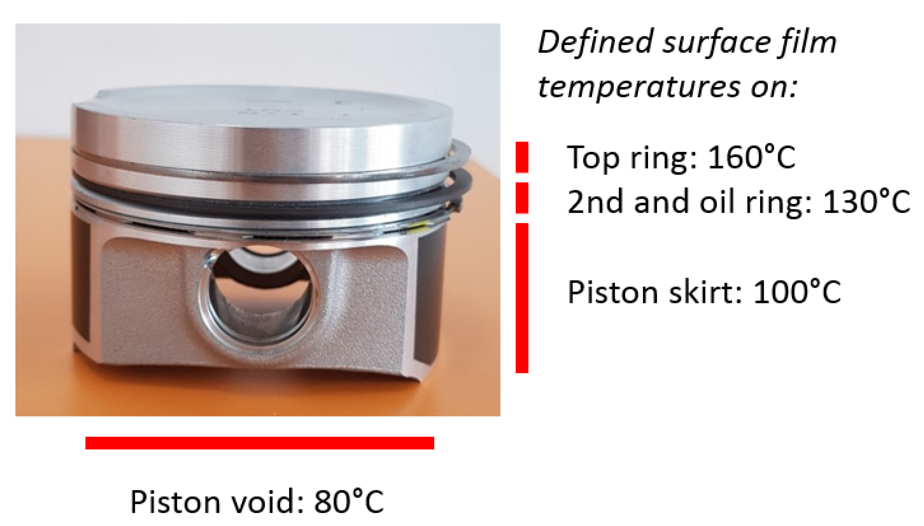
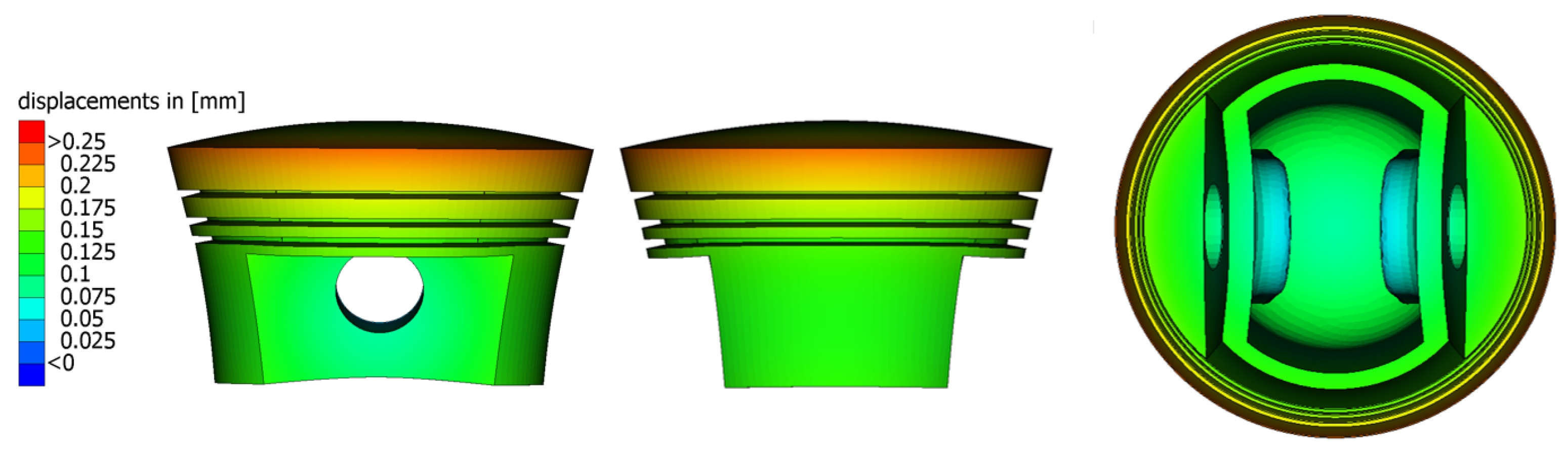
2.3. Thermoelastic Simulation of the Piston
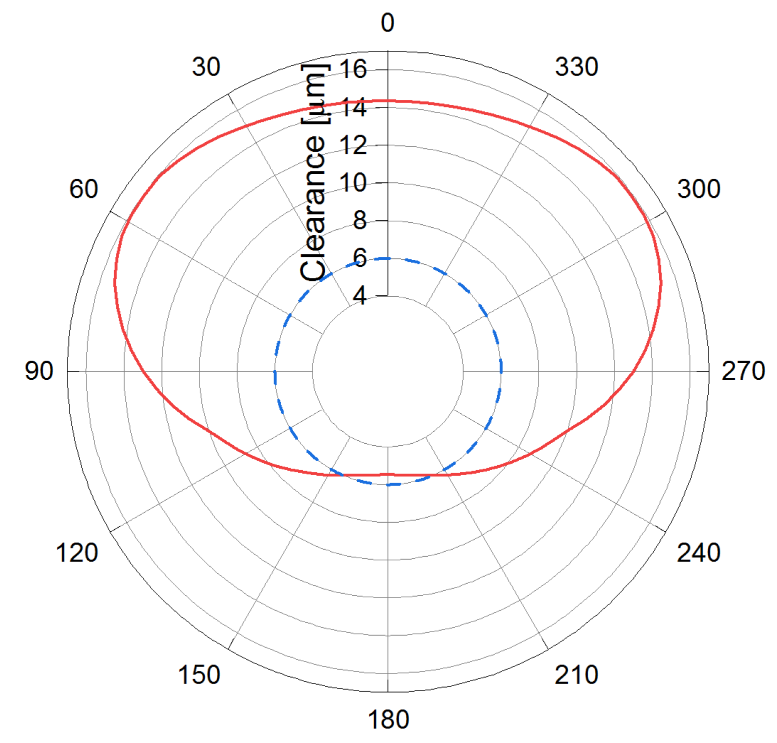
2.4. Simulation of the Piston Pin
3. Causes of Changing Piston-Pin Dynamics
4. Piston-Pin Dynamics and Lubrication for Different Engine Operating Conditions
5. Influence of Piston-Pin Clearance
6. Influence of Piston-Pin Surface Roughness
7. Conclusions
Author Contributions
Funding
Acknowledgments
Conflicts of Interest
References
- Open Access Publisher Intech. Available online: www.intech.com (accessed on 9 March 2020).
- Simulia. Available online: www.simulia.com (accessed on 9 March 2020).
- Shi, F. An analysis of floating piston pin. SAE Int. J. Engines 2011, 4, 2100–2105. [Google Scholar] [CrossRef]
- Ligier, J.L.; Ragot, P. Piston pin: Wear and rotating motion. SAE Trans. 2005, 114, 760–768. [Google Scholar]
- Fridman, V.; Piraner, I.; Clark, K. Modeling of mixed lubrication conditions in a heavy duty piston pin joint. In Proceedings of the ASME 2006 Internal Combustion Engine Division Spring Technical Conference, American Society of Mechanical Engineers Digital Collection, Aachen, Germany, 7–10 May 2006; pp. 741–748. [Google Scholar]
- Suhara, T.; Ato, S.; Takiguchi, M.; Furuhama, S. Friction and Lubrication Characteristics of Piston Pin Boss Bearings of an Automotive Engine; Technical Report, SAE Technical Paper; SAE International: Warrendale, PA, USA, 1997. [Google Scholar]
- Wachtmeister, G.; Hubert, A. Rotation of a piston pin in the small connecting rod eye during engine operation. MTZ Worldw. 2008, 69, 52–57. [Google Scholar] [CrossRef]
- Iwasaki, H.; Higasa, Y.; Takiguchi, M.; Sue, S.; Shishido, K. Effects of Design for Piston Pin and Bearing on State of Bearing Lubrication. In Proceedings of the ASME 2007 Internal Combustion Engine Division Fall Technical Conference, American Society of Mechanical Engineers Digital Collection, Charleston, SC, USA, 14–17 October 2007; pp. 631–636. [Google Scholar]
- Furuhama, S.; Tada, T.; Nakamura, T. Some Measurements of the Piston Temperatures in a Small Type Gasoline Engine. Bull. JSME 1964, 7, 422–429. [Google Scholar] [CrossRef]
- Furuhama, S.; Oya, Y.; Sasaki, H. Temperature measurements of the connecting rod, piston pin and crankpin bearing of an automobile gasoline engine. Bull. JSME 1966, 9, 181–189. [Google Scholar] [CrossRef]
- Furuhama, S.; Enomoto, Y. Piston temperature of automobile gasoline engine in driving on the road. Bull. JSME 1973, 16, 1385–1400. [Google Scholar] [CrossRef]
- Furuhama, S.; Suzuki, H. Temperature distribution of piston rings and piston in high speed diesel engine. Bull. JSME 1979, 22, 1788–1795. [Google Scholar] [CrossRef]
- Sander, D.E.; Allmaier, H.; Priebsch, H.H.; Witt, M.; Skiadas, A. Simulation of journal bearing friction in severe mixed lubrication–Validation and effect of surface smoothing due to running-in. Tribol. Int. 2016, 96, 173–183. [Google Scholar] [CrossRef] [Green Version]
- Knauder, C.; Allmaier, H.; Sander, D.E.; Sams, T. Investigations of the Friction Losses of Different Engine Concepts. Part 2: Sub-assembly resolved friction loss comparison of three engines. Lubricants 2019, 7, 105. [Google Scholar] [CrossRef] [Green Version]
- Knauder, C.; Allmaier, H.; Sander, D.E.; Sams, T. Investigations of the friction losses of different engine concepts. Part 3: Sub-assembly resolved friction reduction potentials and arising risks. Lubricants 2020. submitted. [Google Scholar]
- Allmaier, H.; Priestner, C.; Sander, D.E.; Reich, F. Friction in automotive engines. Tribol. Eng. 2013, 8, 149–184. [Google Scholar]
- Sander, D.E.; Allmaier, H.; Priebsch, H.H. Friction and wear in automotive journal bearings operating in today’s severe conditions. Adv. Tribol. 2016, 7, 143. [Google Scholar]
- Offner, G. Modelling of condensed flexible bodies considering non-linear inertia effects resulting from gross motions. Proc. Inst. Mech. Eng. Part K J. Multi-body Dyn. 2011, 225, 204–219. [Google Scholar] [CrossRef]
- Offner, G. Friction power loss simulation of internal combustion engines considering mixed lubricated radial slider, axial slider and piston to liner contacts. Tribol. Trans. 2013, 56, 503–515. [Google Scholar] [CrossRef]
- Patir, N.; Cheng, H. An average flow model for determining effects of three-dimensional roughness on partial hydrodynamic lubrication. J. Tribol. 1978, 100, 12–17. [Google Scholar] [CrossRef]
- Patir, N.; Cheng, H. Application of average flow model to lubrication between rough sliding surfaces. J. Tribol. 1979, 101, 220–229. [Google Scholar] [CrossRef]
- Jakobsson, B. The finite journal bearing, considering vaporization: Report from the Institute of Machine Elements. Trans. Chalmers Univ. Technol. 1957, 190, 116. [Google Scholar]
- Sander, D.; Allmaier, H.; Priebsch, H.; Reich, F.; Witt, M.; Füllenbach, T.; Skiadas, A.; Brouwer, L.; Schwarze, H. Impact of high pressure and shear thinning on journal bearing friction. Tribol. Int. 2015, 81, 29–37. [Google Scholar] [CrossRef]
- Allmaier, H.; Priestner, C.; Reich, F.; Priebsch, H.; Forstner, C.; Novotny-Farkas, F. Predicting friction reliably and accurately in journal bearings–The importance of extensive oil-models. Tribol. Int. 2012, 48, 93–101. [Google Scholar] [CrossRef]
- Morina, A.; Neville, A. Understanding the composition and low friction tribofilm formation/removal in boundary lubrication. Tribol. Int. 2007, 40, 1696–1704. [Google Scholar] [CrossRef]
- Greenwood, J.; Tripp, J. The contact of two nominally flat rough surfaces. Proc. Inst. Mech. Eng. 1970, 185, 625–633. [Google Scholar] [CrossRef]
- Priestner, C.; Allmaier, H.; Priebsch, H.; Forstner, C. Refined Simulation of Friction Power Loss in Crank Shaft Slider Bearings Considering Wear in the Mixed Lubrication Regime. Tribol. Int. 2012, 46, 200–207. [Google Scholar] [CrossRef]
- Allmaier, H.; Priestner, C.; Reich, F.; Priebsch, H.; Novotny-Farkas, F. Predicting friction reliably and accurately in journal bearings - extending the simulation model to TEHD. Tribol. Int. 2013, 58, 20–28. [Google Scholar] [CrossRef]
- Etsion, I.; Halperin, G.; Becker, E. The effect of various surface treatments on piston pin scuffing resistance. Wear 2006, 261, 785–791. [Google Scholar] [CrossRef]
- Haque, T.; Morina, A.; Neville, A.; Kapadia, R.; Arrowsmith, S. Effect of oil additives on the durability of hydrogenated DLC coating under boundary lubrication conditions. Wear 2009, 266, 147–157. [Google Scholar] [CrossRef]
- Knauder, C.; Allmaier, H.; Sander, D.E.; Sams, T. Investigations of the Friction Losses of Different Engine Concepts. Part 1: A Combined Approach for Applying Subassembly-Resolved Friction Loss Analysis on a Modern Passenger-Car Diesel Engine. Lubricants 2019, 7, 39. [Google Scholar] [CrossRef] [Green Version]
- Zhang, J.; Piao, Z.; Deng, L.; Zhang, S.; Liu, J. Influence of pin assembly on the wear behavior of piston skirt. Eng. Fail. Anal. 2018, 89, 28–36. [Google Scholar] [CrossRef]
- Moshrefi, N.; Mazzella, G.; Yeager, D.; Homco, S. Gasoline Engine Piston Pin Tick Noise; Technical Report, SAE Technical Paper; SAE International: Warrendale, PA, USA, 2007. [Google Scholar]
- Kondo, T.; Ohbayashi, H. Study of Piston Pin Noise of Semi-Floating System; Technical Report, SAE Technical Paper; SAE International: Warrendale, PA, USA, 2012. [Google Scholar]
- Enomoto, Y.; Furuhama, S.; Minakami, K. Heat loss to combustion chamber wall of 4-Stroke gasoline engine: 1st report, heat loss to piston and cylinder. Bull. JSME 1985, 28, 647–655. [Google Scholar] [CrossRef]
- Morel, T.; Keribar, R.; Harman, S. Detailed analysis of heat flow pattern in a piston. In Proceedings of the International Symposium COMODIA, Kyoto, Japan, 3–5 September 1990; Volume 90, pp. 309–314. [Google Scholar]


| Parameter | Gasoline-Engine 1 |
|---|---|
| Volume displacement | 1781 cm |
| Compression ratio | 9.5:1 |
| Bore | 81 mm |
| Stroke | 86.4 mm |
| Nominal torque | 235 Nm |
| Nominal Power | 130 kW |
| Specific power | 72 kW/L |
| Maximum Speed | 6600 rpm |
| Piston pin outer diameter | 20 mm |
| Piston pin inner diameter | 12 mm |
| Piston pin nominal radial clearance | 6 m |
| Piston pin length | 68 mm |
| Piston boss length | 20 mm |
| Small end length | 25 mm |
| Con-rod length | 144 mm |
| Main bearing diameter | 54 mm |
| Main bearing width | 22 mm |
| Main bearing clearance (cold) | 20 m |
| Big-End bearing diameter | 47.8 mm |
| Big-End bearing width | 25 mm |
| SAE class | 5W30 |
| Density at 15 C | 853 kg/m |
| Dynamic viscosity at 40 C | 59.88 mPas |
| Dynamic viscosity at 100 C | 9.98 mPas |
| HTHS viscosity | 3.57 mPas |
| Reference | Variant 1 | Variant 2 | Variant 3 | |
|---|---|---|---|---|
| Surface roughness piston pin | 0.06 m | 0.06 m | 0.06 m | 0.02 m |
| (Cold) Clearance piston pin | 6 m | 4 m | 9 m | 6 m |
| A | 0.064 | mPa s |
| B | 1124.7 | C |
| C | 125.48 | C |
| m | 0.79 | - |
| 0.0009 | 1/bar | |
| r | 0.75 | - |
| K | 3.5 e-7 | s |
| 853 | kg | |
| 15 | C | |
| 0.001 | 1/MPa | |
| 0.003 | 1/MPa | |
| 8.5 | 1/C |
| Engine Speed | Engine Load | Peak Cylinder Pressure |
|---|---|---|
| 1000 rpm | half load | 40 bar |
| 1000 rpm | WOT/full load | 80 bar |
| 3000 rpm | half load | 40 bar |
| 3000 rpm | WOT/full load | 80 bar |
| 6000 rpm | half load | 40 bar |
| 6000 rpm | WOT/full load | 80 bar |
© 2020 by the authors. Licensee MDPI, Basel, Switzerland. This article is an open access article distributed under the terms and conditions of the Creative Commons Attribution (CC BY) license (http://creativecommons.org/licenses/by/4.0/).
Share and Cite
Allmaier, H.; Sander, D.E. Piston-Pin Rotation and Lubrication. Lubricants 2020, 8, 30. https://doi.org/10.3390/lubricants8030030
Allmaier H, Sander DE. Piston-Pin Rotation and Lubrication. Lubricants. 2020; 8(3):30. https://doi.org/10.3390/lubricants8030030
Chicago/Turabian StyleAllmaier, Hannes, and David E. Sander. 2020. "Piston-Pin Rotation and Lubrication" Lubricants 8, no. 3: 30. https://doi.org/10.3390/lubricants8030030
APA StyleAllmaier, H., & Sander, D. E. (2020). Piston-Pin Rotation and Lubrication. Lubricants, 8(3), 30. https://doi.org/10.3390/lubricants8030030