Profile Optimization of Hydraulic, Polymeric, Sliding Seals by Minimizing an Objective Function of Leakage, Friction and Abrasive Wear


Abstract
:
1. Introduction
2. Mathematical Analysis
2.1. Elastohydrodynamics
2.2. Sealing Performance Evaluators
- (a)
- Proposed models of polymer-metal abrasive wear in the literature are empirical/semi-empirical and rely on experimentally determined coefficients. They are thus tight to specific materials and sealed fluids. For example, the trend of the results may be different if water is used as sealed fluid instead of, say, hydraulic oil. There are secondary parameters to consider here such as fluid uptake by the seals, chemical compatibility of polymers and hydraulic fluids, generation of wear debris and others that hinder a precise, quantitative formulation of polymeric abrasive wear [3,4,9,32].
- (b)
- A dynamic modification of seal dimensions by abrasive wear would inevitably have to be linked to a sliding distance (say S) of the contact. But in that case, the so-derived “optimum” seal would be linked to the given S for which the optimization was done in the first place. This means that sealing performance for distances smaller or greater than S would not be optimal. Essentially, we would end up with a seal that not only is designed on the basis of a potentially restrictive abrasive-wear model but also a seal that is designed to operate “optimally” on average for a specific sliding distance S, no more and no less than S. This does not seem plausible or even beneficial for flexible and interactive elements such as polymeric seals that are dynamically affected by many factors during their operation and throughout their service life [9], even off their normal duty cycle.
2.3. Objective Function of Sealing Performance and Optimization
2.4. Necessary and Sufficient Conditions for a Minimum
- (a)
- the Euler-Lagrange equation (Equation (36))
- (b)
- the strengthened Legendre condition or the Weierstrass condition (see Equation (49));
- (c)
- Jacobi’s condition, which requires that Jacobi’s Equation (53) has a solution u that is nonzero for all .
2.5. Solid and Contact Mechanics
Application to a Rectangular-Rounded Seal
3. Application Example
3.1. Input Data
3.2. Results
4. Discussion and Conclusions
Funding
Conflicts of Interest
Nomenclature
| A | apparent area of the sealing contact (Equation (18)) |
| Aa | area of asperity contact (Equation (14)) |
| A1 … A5 | functions (Equations (39)–(43)) |
| b1, b2, b3 | constants (Equations (83), (84) and (86), respectively) |
| B | dummy variable (Equation (31)) |
| c | integration constant (Equation (2)) |
| cr, cs, cf | nonretarded Hamaker constants of the rod, seal and sealed fluid, respectively |
| cτ1, cτ2 | coefficients of the shear strength function |
| c4 | dummy variable (Equation (44)) |
| d1, d2 | arbitrary constants (d1 ≠ 0) |
| D | constant |
| Da | boundary film thickness at asperity junctions |
| E | Weierstrass excess function (Equation (49)) |
| Er, Es | elastic modulus of the rod and the seal, respectively |
| f | function (Equation (19)) |
| F | friction force (Equation (21)) |
| Fa, Fh | asperity (Equation (24) and hydrodynamic (Equation (22) friction force, respectively |
| friction-force representative performance-evaluator (Equation (25)) | |
| Fu | maximum acceptable friction force |
| g | objective function of sealing performance (Equations (29) and (30)) |
| G | function (Equation (34)) |
| Gij, | functions; refer to Equation (57)–(64) |
| Gs | shear modulus of the seal (Equation (78)) |
| h, have | film thickness and its average value, respectively |
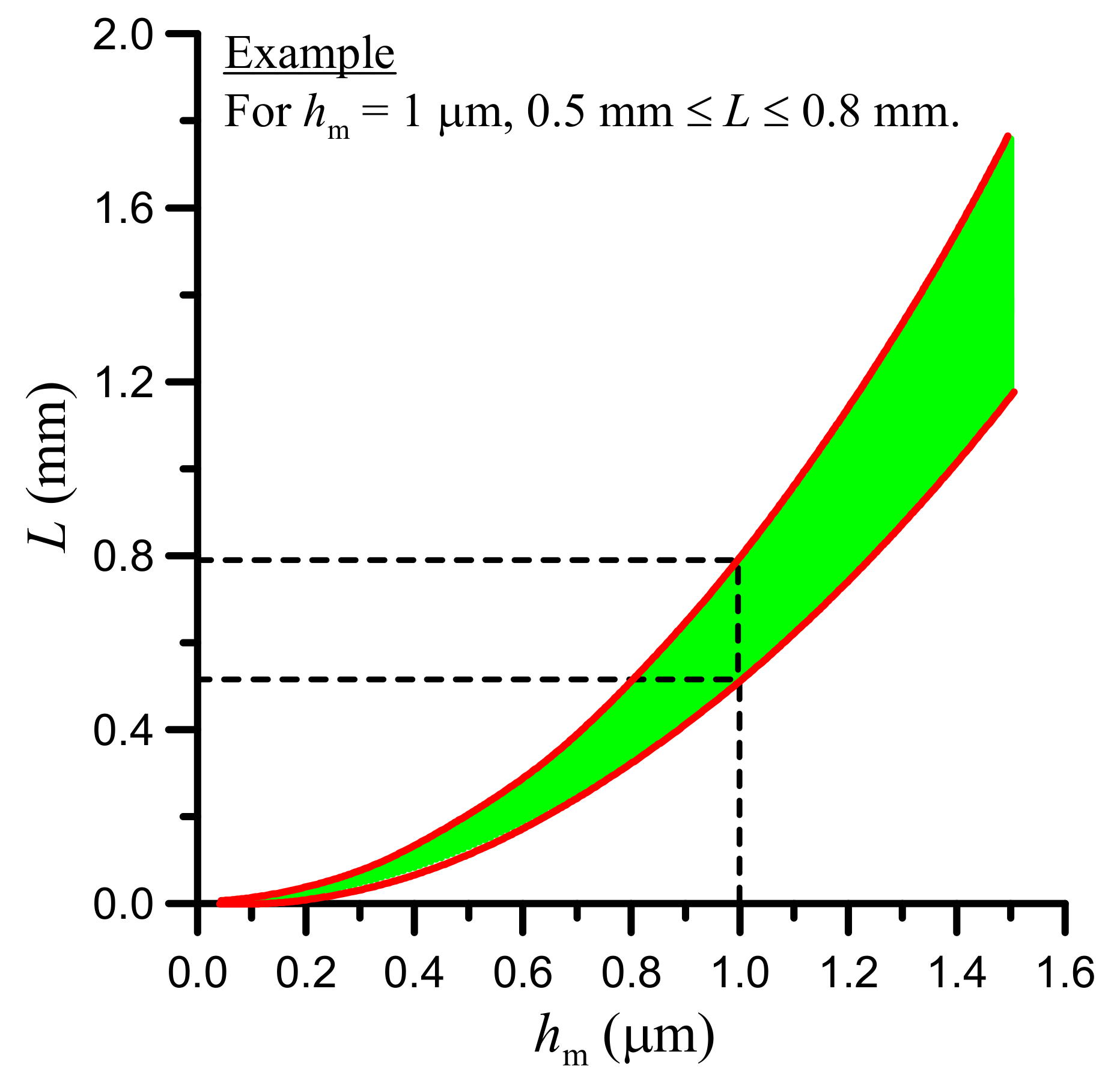
| hm | h at x = xm |
| H | product ρh (Equation (3)) |
| Hm | H at x = xm (Equation (5)) |
| I, J | functionals (Equations (32) and (33), respectively) |
| k1, k2 | coefficients (Equations (74) and (73), respectively) |
| K | constant (Equation (70)) |
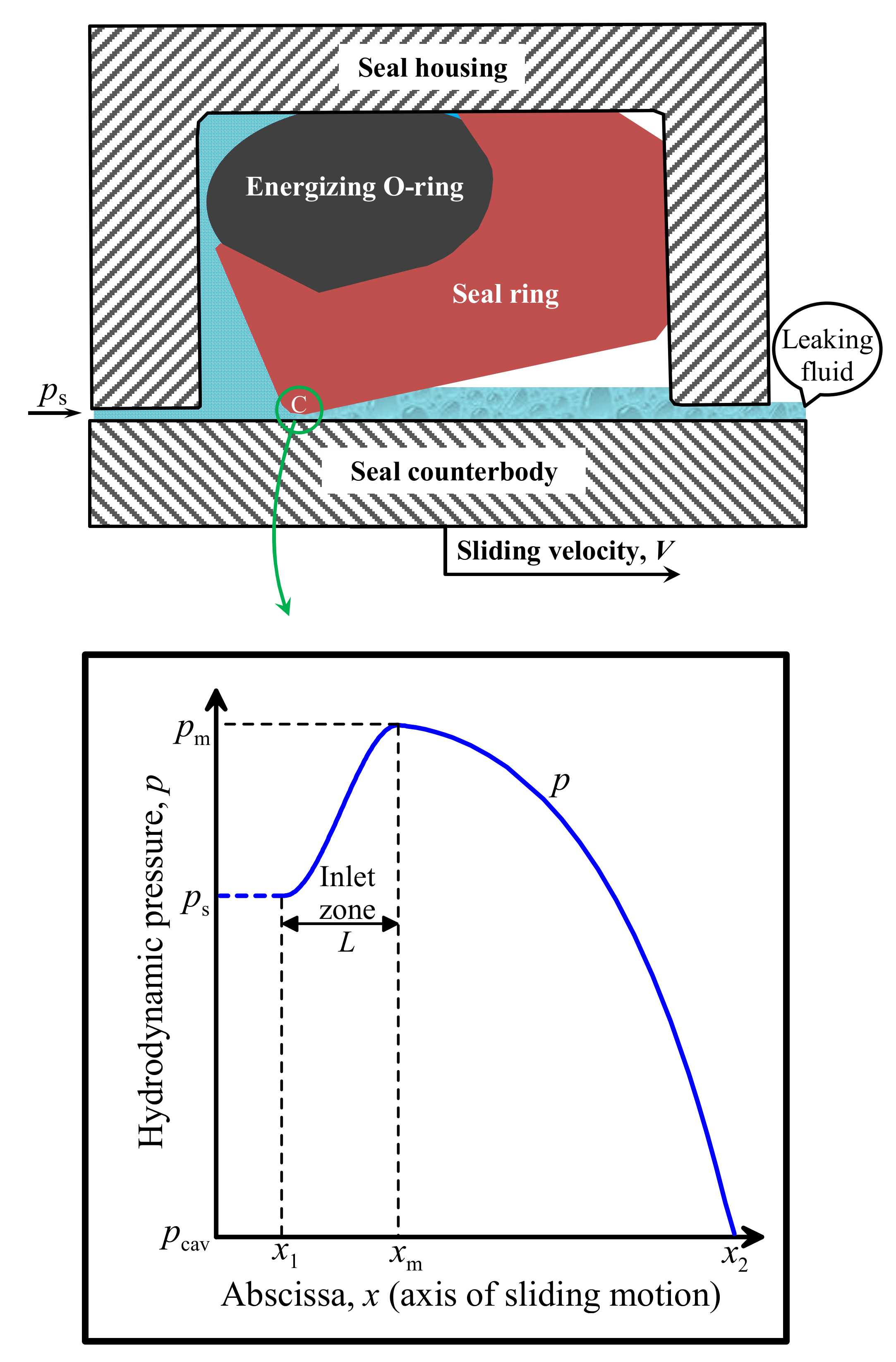
| L | length of the inlet zone (Figure 2) |
| n | parameter equal to either 1, 2 or 5/2 |
| p, | hydrodynamic pressure and its average value, respectively |
| pa | average asperity contact pressure (Equation (12)) |
| pc, | total contact pressure (Equation (71)) and its average value, respectively |
| pcav | cavitation pressure |
| pm | maximum hydrodynamic pressure at the exit of the inlet zone (Figure 2) |
| ps | sealed pressure (Figure 2) |
| q | variable defined through its derivative in Equation (3) |
| Q, Qu | mass leakage rate (Equation (20)) and its maximum acceptable value, respectively |
| r | radius of curvature (Equation (87)) |
| ra | average radius of curvature of roughness asperity tips |
| R | outer radius of the rod |
| sa | surface density of roughness asperities |
| svdW | van der Waals stress (Equation (15)) |
| S02 | ASTM slope of the sealed fluid between 40 and 100 °C, divided by 0.2 (Equation (9)) |
| u | vector |
| uz | normal (radial) surface displacement of the seal (Equation (85)) |
| u1, u2, u3 | elements of vector u |
| V | sliding velocity (Figure 2) |
| wt | wear term (Equation (26)) |
| W | width of the seal along its axis of symmetry |
| Wa | contact load supported by roughness asperities (Equation (13)) |
| x | axial coordinate (Figure 2) |
| xinf | abscissa of the inflexion point of q in the inlet zone |
| xm | abscissa of the point of maximum hydrodynamic pressure (Figure 2) |
| x1, x2 | abscissa of the entry and exit point of the sealing contact, respectively (Figure 2; Equation (75)) |
| Y | vector |
| Y0 | stationary (critical) vector of functional J |
| Greek Symbols | |
| α | pressure-viscosity coefficient of the sealed fluid (Equation (8)) |
| ε | infinitesimal number |
| average axial strain of the seal (Equation (79)) | |
| εz, | radial strain of the seal (Equation (82)) and its average value (Equation (80)), respectively |
| η, ηinf | dynamic viscosity of the sealed fluid (Equation (7)) and its value at x = xinf, respectively |
| η0 | η at atmospheric pressure and local temperature |
| θ | operating temperature |
| λ | Lagrange multiplier, a function of x (Equation (45)) |
| λs | Lamé constant (Equation (77)) |
| Λ | lambda ratio (Equation (16)) |
| νr, νs | Poisson’s ratios of the rod and the seal |
| ν40, ν100 | kinematic viscosities of the sealed fluid at 40 and 100 °C in mm2/s |
| Π | product saraσ |
| ρ | mass density of the sealed fluid (Equation (6)) |
| ρinf, ρm | ρ at x = xinf and at x = xm, respectively |
| ρ0 | ρ at atmospheric pressure and local temperature |
| σ | composite RMS roughness of the sealing surfaces (Equation (17)) |
| σr, σs | RMS roughness (rod, seal) |
| σz | radial stress of the seal in the sealing contact (Equation (76)) |
| τL | limiting shear stress (Equation (23)) |
| τs | shear strength of the sealing ring, (θ in °C; τs in Pa) |
| τ0 | limiting shear stress of the sealed fluid at atmospheric pressure and operating temperature |
| υ | variation of G |
| Abbreviations | |
| ASTM | American Society for Testing and Materials |
| EHD | elastohydrodynamic |
| inf | inflexion (referring to the inflexion point of q) |
| RMS | root mean square |
| sup | supremum (standard mathematical definition) |
References
- Hydraulic Seals–Linear; Trelleborg Sealing Solutions: Trelleborg, Sweden, 2017.
- Flitney, R. Seals and Sealing Handbook, 6th ed.; Chapter 4; Butterworth-Heinemann: Oxford, UK, 2014; ISBN 9780080994161. [Google Scholar]
- Nikas, G.K. Eighty years of research on hydraulic reciprocating seals: Review of tribological studies and related topics since the 1930s. Proc. IMechE Part J. J. Eng. Tribol. 2010, 224, 1–23. [Google Scholar] [CrossRef]
- Nikas, G.K. Research on the tribology of hydraulic reciprocating seals. In Tribology Research Trends; Chapter 1; Hasegawa, T., Ed.; Nova Science Publishers: New York, NY, USA, 2008; ISBN 9781604569124. [Google Scholar]
- Nikas, G.K. Fundamentals of Sealing and Tribology of Hydraulic Reciprocating Seals. In Proceedings of the IMechE 1-Day Seminar “Focus on Reciprocating Seals”, London, UK, 25 June 2008; Available online: http://www.tribology.me.uk/Nikas_IMechE_25-06-2008.pdf (accessed on 2 April 2020).
- Müller, H.K.; Nau, B.S. Fluid Sealing Technology: Principles and Applications; Marcel Dekker Inc.: New York, NY, USA, 1998; ISBN 0824799690. [Google Scholar]
- Nikas, G.K. Fast performance-analysis of rectangular-rounded hydraulic reciprocating seals: Mathematical model and experimental validation at temperatures between –54 and +135 °C. Tribol. Int. 2018, 128, 34–51. [Google Scholar] [CrossRef]
- Nikas, G.K. Parametric and optimization study of rectangular-rounded, hydraulic, elastomeric, reciprocating seals at temperatures between –54 and +135 °C. Lubricants 2018, 6, 77. [Google Scholar] [CrossRef] [Green Version]
- Nikas, G.K. Friction and Wear of Seals. In ASM Handbook, Volume 18: Friction, Lubrication, and Wear Technology; Totten, G., Ed.; ASM International: Ohio, OH, USA, 2017; pp. 957–968. ISBN 9781627081412. [Google Scholar] [CrossRef]
- Nikas, G.K.; Sayles, R.S. Modelling and optimization of composite rectangular reciprocating seals. Proc. IMechE—Part J. J. Eng. Tribol. 2006, 220, 395–412. [Google Scholar] [CrossRef]
- Nikas, G.K.; Burridge, G.; Sayles, R.S. Modelling and optimization of rotary vane seals. Proc. IMechE—Part J. J. Eng. Tribol. 2007, 221, 699–715. [Google Scholar] [CrossRef]
- Field, G.J.; Nau, B.S. A theoretical study of the elastohydrodynamic lubrication of reciprocating rubber seals. Trans. ASLE 1975, 18, 48–54. [Google Scholar] [CrossRef]
- Johannesson, H.L. Oil leakage and friction forces of reciprocating O-ring seals considering cavitation. ASME J. Lubr. Technol. 1983, 105, 288–296. [Google Scholar] [CrossRef]
- Karaszkiewicz, A. Hydrodynamics of rubber seals for reciprocating motion. Ind. Eng. Chem. Prod. Res. Dev. 1985, 24, 283–289. [Google Scholar] [CrossRef]
- Karaszkiewicz, A. Hydrodynamics of rubber seals for reciprocating motion, lubricating film thickness, and out-leakage of O-seals. Ind. Eng. Chem. Prod. Res. Dev. 1987, 26, 2180–2185. [Google Scholar] [CrossRef]
- Kanters, A.F.C. On the Calculation of Leakage and Friction of Reciprocating Elastomeric Seals. Ph.D. Thesis, Eindhoven University of Technology, Eindhoven, The Netherlands, 1990. [Google Scholar] [CrossRef]
- Kanters, A.F.C.; Verest, J.F.M.; Visscher, M. On reciprocating elastomeric seals: Calculation of film thicknesses using the inverse hydrodynamic lubrication theory. STLE Tribol. Trans. 1990, 33, 301–306. [Google Scholar] [CrossRef]
- Salant, R.F.; Maser, N.; Yang, B. Numerical model of a reciprocating hydraulic rod seal. ASME J. Tribol. 2007, 129, 91–97. [Google Scholar] [CrossRef]
- Grimble, D.; Theodossiades, S.; Rahnejat, H.; Wilby, M. Tribology of rough ultra-film contacts in drug delivery devices. Proc. IMechE—Part C J. Mech. Eng. Sci. 2008, 222, 2209–2216. [Google Scholar] [CrossRef] [Green Version]
- Yang, B.; Salant, R.F. Soft EHL simulations of U-cup and step hydraulic rod seals. ASME J. Tribol. 2009, 131, 021501. [Google Scholar] [CrossRef]
- Yang, B.; Salant, R.F. Elastohydrodynamic lubrication simulation of O-ring and U-cup hydraulic seals. Proc. IMechE—Part J. J. Eng. Tribol. 2011, 225, 603–610. [Google Scholar] [CrossRef]
- Fatu, A.; Hajjam, M. Numerical modelling of hydraulic seals by inverse lubrication theory. Proc. IMechE—Part J. J. Eng. Tribol. 2011, 225, 1159–1173. [Google Scholar] [CrossRef]
- Nikas, G.K.; Sayles, R.S. Study of leakage and friction of flexible seals for steady motion via a numerical approximation method. Tribol. Int. 2006, 39, 921–936. [Google Scholar] [CrossRef]
- Békési, N. Friction and Wear of Elastomers and Sliding Seals. Ph.D. Thesis, Department of Machine and Product Design, Faculty of Mechanical Engineering, Budapest University of Technology and Economics, Budapest, Hungary, 2011. [Google Scholar]
- Alkadhimi, F. Wear Testing and Finite Element Analysis of Nitrile Rubber (NBR) Hand Pump Seals. M.Eng. Thesis, School of Mechanical and Manufacturing Engineering, Dublin City University, Dublin, Ireland, 2015. [Google Scholar]
- Bhaumik, S.; Kumaraswamy, A.; Guruprasad, S.; Bhandari, P. Study of effect of seal profile on tribological characteristics of reciprocating hydraulic seals. Tribol. Ind. 2015, 37, 264–274. [Google Scholar]
- Dowson, D.; Higginson, G.R. Elasto-Hydrodynamic Lubrication: The Fundamentals of Roller and Gear Lubrication; Pergamon Press: Oxford, UK, 1966. [Google Scholar]
- Barus, C. Isothermals, isopiestics, and isometrics relative to viscosity. Am. J. Sci. 1893, 45, 87–96. [Google Scholar] [CrossRef]
- Wu, C.S.; Klaus, E.E.; Duda, J.L. Development of a method for the prediction of pressure-viscosity coefficients of lubricating oils based on free-volume theory. ASME J. Tribol. 1989, 111, 121–128. [Google Scholar] [CrossRef]
- Denis, J.; Briant, J.; Hipeaux, J.C. Lubricant Properties, Analysis and Testing; Section 2.5.5.1; Editions Technip: Paris, France, 2000; ISBN 2710807467. [Google Scholar]
- Greenwood, J.A.; Tripp, J.H. The contact of two nominally flat rough surfaces. Proc. IMechE 1970, 185, 625–633. [Google Scholar] [CrossRef]
- Zhang, S.-W. Tribology of Elastomers; Elsevier: London, UK, 2004; ISBN 0444513183. [Google Scholar]
- Hamrock, B.J.; Schmid, S.R.; Jacobson, B.O. Fundamentals of Fluid Film Lubrication, 2nd ed.; Section 3.9; Marcel Dekker, Inc.: New York, NY, USA, 2004; ISBN 0824753712. [Google Scholar]
- Komzsik, L. Applied Calculus of Variations for Engineers, 2nd ed.; CRC Press: New York, NY, USA, 2014; ISBN 9781482253597. [Google Scholar]
- Kot, M. A First Course in the Calculus of Variations; Series: Student Mathematical Library; American Mathematical Society: Providence, RI, USA, 2014; Volume 72, ISBN 9781470414955. [Google Scholar]
- Gregory, J.; Lin, C. Constrained Optimization in the Calculus of Variations and Optimal Control Theory; Chapman & Hall: London, UK, 1992; ISBN 9789401052955. [Google Scholar]
- SSL II User’s Guide (Scientific Subroutine Library); Fujitsu Ltd.: Tokyo, Japan, 1998.
- Gelfand, I.M.; Fomin, S.V. Calculus of Variations; Prentice Hall, Inc.: Englewood Cliffs, NJ, USA, 1963. [Google Scholar]
- O’Neil, P.V. Advanced Engineering Mathematics, 7th ed.; Cengage: Stamford, CT, USA, 2012; ISBN 9781111427412. [Google Scholar]
- Wazwaz, A.-M. The variational iteration method for analytic treatment for linear and nonlinear ODEs. Appl. Math. Comput. 2009, 212, 120–134. [Google Scholar] [CrossRef]
- Polyanin, A.D.; Manzhirov, A.V. Handbook of Integral Equations, 2nd ed.; Section 13.2.1; Chapman & Hall/CRC: New York, NY, USA, 2008; ISBN 9781584885078. [Google Scholar]
- Nikas, G.K.; Sayles, R.S. Nonlinear elasticity of rectangular elastomeric seals and its effect on elastohydrodynamic numerical analysis. Tribol. Int. 2004, 37, 651–660. [Google Scholar] [CrossRef]
- Johnson, K.L. Contact Mechanics; Cambridge University Press: Cambridge, UK, 1985; ISBN 0521347963. [Google Scholar]
- Nikas, G.K.; Almond, R.V.; Burridge, G. Experimental study of leakage and friction of rectangular, elastomeric hydraulic seals for reciprocating motion from –54 to +135 °C and pressures from 3.4 to 34.5 MPa. Tribol. Trans. 2014, 57, 846–865. [Google Scholar] [CrossRef]
- Jacobson, B. A high pressure-short time shear strength analyzer for lubricants. ASME J. Tribol. 1985, 107, 220–223. [Google Scholar] [CrossRef]
- Prokopovich, P.; Theodossiades, S.; Rahnejat, H.; Hodson, D. Friction in ultra-thin conjunction of valve seals of pressurised metered dose inhalers. Wear 2010, 268, 845–852. [Google Scholar] [CrossRef] [Green Version]
- Israelachvili, J.N. Intermolecular and Surface Forces, 3rd ed.; Academic Press (Elsevier): Oxford, UK, 2011; ISBN 9780123919274. [Google Scholar]
- Nikas, G.K. Determination of Polymeric Sealing Principles for End User High Reliability; Technical Report DOW-08/01; Department of Mechanical Engineering, Tribology Group, Imperial College: London, UK, 2001; Available online: www.tribology.me.uk/project5.htm (accessed on 2 April 2020).
- Stupkiewicz, S.; Marciniszyn, A. Elastohydrodynamic lubrication and finite configuration changes in reciprocating seals. Tribol. Int. 2009, 42, 615–627. [Google Scholar] [CrossRef]
- Öngün, Y.; André, M.; Bartel, D.; Deters, L. An axisymmetric hydrodynamic interface element for finite-element computations of mixed lubrication in rubber seals. Proc. IMechE—Part J. J. Eng. Tribol. 2008, 222, 471–481. [Google Scholar] [CrossRef]


| Input Data for the Numerical Model | Values |
|---|---|
| Sealed fluid | MIL-H-5606 (Nikas et al. [44]) |
| Outer radius of the rod: R (mm) | 15 |
| Width of the seal: W (mm) | 3 |
| Elastic modulus: Er; Es (–0.1 ≤ εz ≤ 0) (MPa) | 207 × 103; 7 |
| Poisson’s ratio: νr; νs | 0.30; 0.499 |
| Sealed pressure: ps (MPa) | 10 |
| Maximum elastohydrodynamic pressure: pm (MPa) | 15 |
| Cavitation pressure: pcav (kPa) | 101 (1 atm) |
| Sliding velocity: V (m/s) | 0.5 |
| Operating temperature: θ (°C) | 23 |
| Mass density of the sealed fluid at atmospheric pressure: ρ0 (kg/m3) | 842.2 |
| Dynamic viscosity of the sealed fluid at atmospheric pressure: η0 (Pa·s) | |
| Pressure-viscosity coefficient: α (GPa–1) | 14.8 (computed by Equation (8)) |
| Limiting shear stress of the sealed fluid at atmospheric pressure: τ0 (MPa) | 4 (Jacobson [45]) |
| Average radius of curvature of asperity tips: ra (μm) | 1.5 (Prokopovich et al. [46]) |
| Boundary film thickness at asperity junctions: Da (nm) | 2 (estimated; Israelachvili [47]) |
| Nonretarded Hamaker constants: cr; cs; cf (J × 10–20) | 40.0; 8.6; 5.0 (Israelachvili [47]) |
| RMS roughness: σr; σs (μm) | 0.07; 1.70 |
| Product Π = saraσ | 0.12 (Nikas [7,8]) |
| Coefficients of the shear strength function of the seal: cτ1 (1/°C); cτ2 | –0.0090729; 16.0829302 a |
| Maximum acceptable mass leakage rate: Qu (mg/s) | 30 |
| Maximum acceptable friction force: Fu (N) | 80 |
© 2020 by the author. Licensee MDPI, Basel, Switzerland. This article is an open access article distributed under the terms and conditions of the Creative Commons Attribution (CC BY) license (http://creativecommons.org/licenses/by/4.0/).
Share and Cite
Nikas, G.K. Profile Optimization of Hydraulic, Polymeric, Sliding Seals by Minimizing an Objective Function of Leakage, Friction and Abrasive Wear. Lubricants 2020, 8, 40. https://doi.org/10.3390/lubricants8040040
Nikas GK. Profile Optimization of Hydraulic, Polymeric, Sliding Seals by Minimizing an Objective Function of Leakage, Friction and Abrasive Wear. Lubricants. 2020; 8(4):40. https://doi.org/10.3390/lubricants8040040
Chicago/Turabian StyleNikas, George K. 2020. "Profile Optimization of Hydraulic, Polymeric, Sliding Seals by Minimizing an Objective Function of Leakage, Friction and Abrasive Wear" Lubricants 8, no. 4: 40. https://doi.org/10.3390/lubricants8040040
APA StyleNikas, G. K. (2020). Profile Optimization of Hydraulic, Polymeric, Sliding Seals by Minimizing an Objective Function of Leakage, Friction and Abrasive Wear. Lubricants, 8(4), 40. https://doi.org/10.3390/lubricants8040040