Studies on the Pressure Buildup and Shear Flow Factors in the Cavitation Regime


Institut für Dynamik und Schwingungen, Technische Universität Braunschweig, 38106 Braunschweig, Germany
*
Author to whom correspondence should be addressed.
Lubricants 2020, 8(8), 82; https://doi.org/10.3390/lubricants8080082
Submission received: 1 July 2020
/
Revised: 29 July 2020
/
Accepted: 5 August 2020
/
Published: 11 August 2020
Abstract
:Modeling tribological contacts is commonly based on the Reynolds equation. This study discusses the validity of conventional, averaged Reynolds simulations for systems including starvation regimes. Two fundamental assumptions that are used as common practice in many elasto-hydrodynamic (EHD) calculations, are debated. First, the use of a cavitation pressure (in most cases assumed to be zero) independent of the microscopic roughness. Second, the application of a shear flow factor, which is determined on a microscopic scale with a fully filled gap. The validity of these two assumptions is analyzed with simulations on the microscopic scale. For this purpose, simulations of partially filled contacts are carried out using the partially filled gaps model developed by the authors. The topographies, the filling level and the fluid distribution were varied. The simulations comply with established models for the fully filled state and show a distinct behavior for partial filling and different fluid distributions. Neglecting the contribution to pressure buildup and shear flow of partially filled domains is a valid method in most cases. However, as this study shows, near the fully filled regime, the domains should be handled with care.

1. Introduction
Today the modelling of lubricated contacts is still based on the approaches developed by Osbourne Reynolds in 1886 and formulated in the equation named after him [1]. Since then, many different modifications and extensions have been made to this equation, such as the consideration of deformations (e.g., [2]), non-Newtonian fluids (e.g., [3]), mass-preserving cavitation formulations (e.g., [4]) and the implementation of roughness influences (e.g., [5]), to name a few.
Motivated by contact–mechanical studies, this study is dedicated to a rather specific fundamental question: To what extent is multiscale modeling in the cavitation regime applicable? Further information on the motivation is presented and discussed below, followed by a brief description of the used partially filled gaps (PFG) model [6]. In this paper, studies with varying cavitation degrees and different fluid distributions are carried out and evaluated.
1.1. Motivation
The starting point of this study is the fundamental question from contact mechanics, how the tribological properties of a mechanical contact change, if fluids are involved. The transition from a dry contact to a fully filled contact is a very complex problem. This transition can occur when dry contacts experience wetting (for example a wet car brake), but it can also occur during machine idling (e.g., of turbines) and emergency operation conditions (e.g., oil supply failure). These starved systems all have in common that the fluid strongly influences the gap but does not fully fill it. This regime is not yet fully understood, and this study aims to contribute to the understanding of partially filled gaps, especially for systems where the filling level is significantly below 100%. In the context of this study the filling level will be the ratio of fluid volume to gap volume.
As stated before, the problem in this study is especially focused on the classification and quantification of the influence of the amount of fluid in the gap (see Figure 1). In this picture the emphasis should not be on how the fluid is distributed in the vertical z-direction, but rather in the gap plane directions (x and y).
The fact that the volume present in the gap can be used to generate the transition from dry friction () to hydrodynamic friction () is obvious, but a systematic quantification of the relation between fluid volume and the friction regime has not yet been carried out.
For this purpose, the authors of this paper have experimentally investigated the correlation between the fluid volume and the resulting coefficient of friction as well as the gap height using a specific test rig, as published in [7]. This showed a “Stribeck-like” behavior with the variation of the fluid quantity (for small values the friction coefficient decreased until reaching a minimum, for higher values the friction coefficient increased with increasing fluid volume), see Figure 2b. However, the quantitative variation differs from the variation due to increasing velocities. For example, a halving of the fluid quantity led to a stronger decrease of the coefficient of friction than a halving of the velocity [7].
In addition to the coefficient of friction, the flow behavior of the fluid for varying rotational speeds and viscosities was also investigated (see Figure 2b). It became clear that in this experiment a hydrodynamic friction regime was correlated with a ring-shaped fluid distribution (e.g., top right), while a rather dry friction regime was associated with the formation of fluidic “islands” (e.g., bottom left).
This led to the conclusion that not only the amount of fluid itself influences the tribological properties, but also its distribution within the contact. In the context of a micro-elastohydrodynamic (micro-EHD) simulation the filling level is a value which represents the integral portion of the fluid in the control volume concerned. The distribution of the fluid on the microscopic level is usually not considered.
The assumption that the integral volume is the decisive measure, rather than its distribution may be justified for many applications, but its general validity should also be evaluated in this paper. For this purpose, this paper includes comparisons of micro-EHD simulations under starvation where the influence of the fluid distribution is considered. The primary goal of these investigations is to show the opportunities and limits of the conventional micro-EHD approach for this special case. First and foremost, the results should serve the characterization of contact mechanical problems.
1.2. Common Assumptions and Realization of the micro-EHD Problem
The basis for the following study is the well-known Reynolds equation under consideration of microscopic surface roughness. This multiscale modeling technique, (for this application known as “micro-EHD simulation”), is usually represented in literature in the following form (see Equation (1)):
Therein, denotes the pressure, the gap height on the macroscale, and the fluid’s density and dynamic viscosity, and the velocity of the lower and upper surface in x-direction and and the velocity of the lower and upper surface in y-direction. The local variable corresponds to the ratio of fluid volume to gap volume and guarantees the conservation of mass. Since fluids can generally only transmit very low tensile stresses, this approach makes it possible to physically describe the tearing off of the lubricant film, especially in diverging gaps. This behavior has also been identified in many studies e.g., [8,9,10,11,12,13,14].
From a mathematical point of view, this procedure results in a complementary system of equations; where the gap is fully filled (), the pressure is unknown, while at the locations of the unknown filling level () the pressure corresponds to the assumed cavitation pressure, which is mostly set to zero. A good overview of the implications of using the filling level as a measure for the local film starvation can be found in [13]. Alternative approaches to solve the Reynolds equation in the cavitation regime can be found in [15].
and denote the pressure flow factors in x- and y-direction and and the shear flow factors in x- and y-direction. The latter four mentioned factors represent the influence of the roughnesses on the microscopic scale, thus modifying the flow on the macroscopic scale.
In this paper, the shear flow factor in x-direction plays a significant role, it is identified by calculating a mean flow through a representative part on the microscopic scale. For this purpose, the Reynolds equation is used on this microscopic domain with specific boundary conditions, as explained later, and the shear flow factor resulting from the simulation can be determined as follows:
where the shear flow factor is normed by a resulting roughness [16]. The shear flow factor depends in particular on the mean gap height on the microscopic scale (i.e., the macroscopic gap height ) and is usually determined in advance of the simulation as a function of and then implemented into the model accordingly.
This results in two fundamental assumptions that are used as common practice in many EHD calculations:
- (1)
- In macroscopically not fully filled areas the pressure corresponds to the cavitation pressure (in most cases assumed to be zero), independent of the microscopic roughness;
- (2)
- In macroscopically not fully filled areas, a shear flow factor is applied, which was determined in advance on a microscopic scale with a fully filled gap.
This paper aims to investigate the validity of these two assumptions with simulations on the microscopic scale.
1.3. PFG Model and Its Application to the Calculation of Pressures and Shear Flow Factors
Before the results of the study will be presented, the modeling technique used is briefly introduced.
The partially filled gaps model developed by the authors is used for this study. Figure 3 illustrates its basic idea. It considers arbitrary topographies of any shape and, most importantly for this study, arbitrary initial fluid distributions. The object of the investigations with this model is in particular the dynamics of the fluid distribution changing over time and the associated tribological properties.
The model has been extensively derived and applied in the references [6,17,18] so that it is only briefly introduced here (see Figure 4). It uses five state variables at each discrete location in the domain: the pressure, the velocities in x- and y-direction, the gap height and the fluid volume. These state variables interact via different constitutive laws. In addition to a simplified form of the Navier–Stokes equations (in 2D), the continuity equation is used, and the pressure is determined using the method of artificial compressibility. This in turn generates deformations, which are calculated using the integrated Boussinesq formula and define the gap heights.
Numerically, this model results in a system of nonlinear implicit algebraic equations that are iteratively solved with the Newton-method. The model technique itself should not be the focus of this paper. In comparison to the Reynolds equation, the equations for the balance of forces and the mass balance are formulated in separate equations, which has certain advantages with regard to the flexibility of the equations and terms used (such as convective components). As in the Reynolds equation, in the PFGM the Navier–Stokes equation is not discretized by the height direction neglecting the flows in z-direction. The flows in the gap directions (x- and y-) are approximated accordingly by quadratic flow profiles over the height. In the present application case of the PFG model, however, the convective terms are neglected due to the relatively small velocities. Thus, the equations used are practically equal to the Reynolds equation under the premise that the squeeze flow term also contains the temporal change of the filling degree . In this context, the local filling degree explicitly depends on time; so that the term would need to be considered, thus each time step being treated as unsteady. With the explicit time dependence of θ, the fluid distribution results from the calculated flows. Mathematically speaking the calculation of the fluid distribution becomes an initial value problem. Therefore, in this study the fluid is distributed at simulation start by a dedicated algorithm (see Section 2.3). This procedure is in contrast to conventional, partial filling models, which are usually implemented as boundary value problems with a boundary condition at the lubricant inlet.
This paper does not primarily focus on the effects of the numeric modeling, but rather on the different results for the microsystem studies with varying global filling ratios. Nevertheless, to prove the validity of the PFG model for this type of problem, the calculation of shear flow factors for fully filled gaps, which is very well documented in the literature, will serve as a reference.
The shear flow factors are determined by the conventional method where the mean flow is determined according to Equation (2) for an area where there are no pressure differences between the boundaries () and where the lower surface has the opposite velocity to the upper surface (). In the following studies, the shear flow factor is always calculated in the x-direction, where flows over the lateral boundaries (in the y-direction at and ) are prevented. The model accounts for solid body contact and the associated elastic deformations. However, the elastic deformation caused by the fluid pressure was neglected. This approach, which is convenient for these studies, represents a material with a high Young’s modulus.
All simulations are performed with Gaussian surfaces with an initial mean square roughness of 2.0 µm (i.e., the standard deviation of the topographies height distribution). The topographies used are similar to the topographies shown in Section 2.1. This study focuses on results for isotropic surfaces (Peklenik factor = 1). Both surfaces were discretized with a 40 × 40 grid. Further studies with finer meshes were performed, these showed no significant change in results [18]. To compare the results, the studies by Patir and Cheng [5,16], Elrod [4], Tripp [19] and Rienäcker [20] are used.
Figure 5 shows the shear flow factors for fully filled gaps, comparing the PFGM results with results gained by the other established approaches. The mean gap height was varied for different topographies, all results were plotted as usual over the ratio .
Various studies showed that the models from Patir/Cheng, Elrod and Tripp are not suitable for low values of . With a more detailed model regarding elastic deformations and solid body contacts Rienäcker was able to compute results near , pointing out the plausible drastic decrease of the flows for values below 1.0 In the present study, only solid body contact was modeled while elastic deformation due to hydrodynamic pressure was neglected. This is a potential reason the PFGM results are higher than the Rienäcker model, but below the other models. Either way, this paper does not want to discuss the differences of the models and instead focuses on the filling level impact. Therefore, systems in the range of are studied. Here, it can be concluded that the PFG model provides results nearly identical to all other methods and is therefore suitable for the studies carried out in the following chapters. The solution for the case of a fully filled gap shown here serves as a reference for quantifying the influence of the degree of partial filling.
For the sake of completeness, it should be mentioned that the PFG model was also used with topographies with Peklenik factors from [0.33 … 4]. These simulations also showed a very good compliance with the models in the literature.
In summary, very little research is available about the influence of the filling level on the shear flow factor. Typically, the flow factor is computed for the fully filled gap. For a great variety of applications, however, a cavitation or partially filled domain exists. Therefore, this work focuses on the influence of different filling degrees and filling states. Bartel [21] suggests that the flow in cavitation domains is strongly influenced by the filling degree.
2. Studies with a Partially Filled Gap
To examine the effect of partial filling on microscopic length scales, a great variety of studies were undertaken by the authors. The variable parameters of the study are the filling level, the topography and the fluid distribution in the gap. The parameter variation will be explained in more detail in this section. For this highly nonlinear problem, especially with partial filling, a scaled (normalized) calculation is not possible. Therefore, exemplary application-oriented system parameters are used. The basic insights gained from this analysis can also be applied to other sets of parameters accordingly.
Both surfaces move with the same velocity, but in contrary directions with and the dynamic viscosity was set to which is common for a cold engine oil. In the simulation, a partially filled cell is assumed to have ambient pressure. The ambient pressure was set to , assuming that a gas phase/air does not lead to pressure buildup. This assumption may not be suitable to all systems, as recent studies from Shen et al. that the cavitation pressure can influence the results, for example with micro textured surfaces [22,23]. It is very complex to determine in advance possible higher local cavitation pressures for these scenarios. For this reason—and to get first insights into the problem—the cavitation pressure was pragmatically set to the common value of . Future studies will address the influence of trapped air and corresponding higher local cavitation pressures. In terms of the global cavitation pressure as an integral pressure over the not fully filled microscopic domain, the present study already provides information.
2.1. Varying the Topography
The topography was varied with ten different randomly created surfaces that were similar regarding their surface roughness and their Peklenik factor. The target value of the surface roughness is and 1.0 for the Peklenik factor. The variance of the properties is shown in Figure 6.
The same ten topographies were used for all simulations in this study. This ensures the comparability between different results and to a certain extent shows the influence of the variety of the results due to the variety of the roughness (for these 10 topographies the standard deviation related to the mean value amounts approximately 10%). As an example, Figure 7 shows the gap height of topography “3”. Here, the gap height is defined as the sum of the nominal gap height and the two surface profiles and . The mean gap height is and thus is in the range of . The length and width of the domain is .
2.2. Varying the Filling Level
A specific location on the macroscopic scale, where in a macro simulation (e.g., of a large plain bearing) a node with θ < 1 is calculated locally, should be an area on the microscopic scale, which should be filled with this filling level on average. With the previously known total gap volume on the microscopic scale the fluid volume can be calculated for the microscopic area with . The filling level was varied with different fluid volumes in the gap. The filling level and thus the fluid volume was always computed in regard to the initial topography. The study varies the filling level from .
2.3. Varying the Initial Fluid Distribution
The filling level does not account for the explicit fluid distribution in the gap. Obviously though, the actual distribution of fluid between the contact partners strongly influences the friction regime.
The actual distribution of the fluid in a partially filled gap can possibly only be determined with a very finely discretized 3D CFD simulation. However, these simulations are subject to considerable requirements, so that a different approach is being taken here. To understand the impact of the fluid distribution, the distribution was varied with different filling procedures (FP). In order to determine the influence of the fluid quantity and fluid distribution on pressure buildup and flow, fluid distributions were chosen to be regarded as extreme for the problem to be investigated. The distributions do not depict realistic distributions, but rather assess the spectrum in which possible variations may occur. This refers to maximum/minimum values for the pressure buildup and the shear flow factor. For this reason, the initial fluid distribution algorithms were designed to either completely fill a particularly large number of cells, completely fill a particularly small number of cells or distribute the fluid very homogeneously or nonhomogeneously (see below). The filling procedures calculate an initial fluid distribution. The movement of the topographies results in flows that interact directly with the occurring fluid distribution.
Five different procedures were designed and used. Each procedure is visualized below with the same topography, a one-dimensional sample that serves as an example and a filling level of 0.7. The total fluid volume in any of the five cases is thus . The cells near the index 20 are in solid body contact. Table 1 introduces the varying filling procedures. In the illustrations, the fluid is plotted at the bottom. However, as in the Reynolds equation with , the model cannot distinguish at what height the fluid is located. The illustrations indicate the horizontal fluid distribution rather than the vertical distribution.
3. Results
All calculations were completed with the PFG model. The simulations for were created without a specific filling procedure because obviously all cells were fully filled initially. The calculations with the filling level of 1 are important to compare and interpret the results with the results of the partial filling. For each configuration one time step was computed. The time step was chosen so that the gap height distribution moved by the length of 1 discrete cell (dx).
3.1. Shear Flow Factor
First, the results are analyzed regarding the shear flow factor. Since the interpretation of the following results is based in particular on the flows under partial filling through the micro-roughness, the associated flow given in Equation (1) is considered here. This correlates to the product of the actual shear flow factor and the mean filling level . According to Equation (1) and Equation (2), the considered value provided in the studies is therefore and for simplicity assigned as “shear flow factor”.
Figure 8 shows the shear flow factor over all filling procedures and filling levels. In order to maintain a clear visualization, the x-axis was plotted nonuniformly and the results for the filling procedures are plotted with a slight offset. Therein, the five different filling procedures are shown with the different colors. A separate color was chosen for the full filling because no specific filling procedure was used. Each diamond represents an individual result of the simulation.
For each filling level and filling procedure ten different simulations were run with the topographies (thus 10 diamonds per filling level and filling procedure). Additionally, the mean values (connected with the lines) and the standard deviation of the shear flow factor are plotted with the corresponding error bar. In the rare case that a simulation did not converge numerically, the respective value is missing (therefore, in very few cases there are less than 10 diamonds).
The variation of the simulation results (error bars) is directly connected to the slight variance in the topography surface properties (compare Figure 6) and is not caused by errors of numeric nature or similar (this conclusion was drawn from a plot of the shear flow factor over the roughness which is not shown here).
First of all, it is noticeable that the variation in roughness (10% standard deviation) is also roughly found in the relative standard deviation of the shear flow factors at larger filling levels (from 0.95), where this measure is in the range between 14% to 17%. For the roughness range investigated here, this indicates a slight nonlinear relationship between roughness and shear flow factor.
All shear flow factors sharply decrease with decreasing filling levels. For two of the filling procedures (FP 3 and FP 4), the absolute value of the shear flow factor decreases to a minimum absolute value of . The reason that the factor does not decrease further is that these fluid distributions have many fully filled cells even at smaller filling levels. The other three filling procedures (FP 1, FP 2 and FP 5) have a minimal shear flow factor close to 0.
When the filling level is reduced from to , the mean shear flow factor changes from −0.519 to a range between −0.365 at FP2 to −0.494 at FP3. This underlines the significance of the transient fluid distribution in the gap. At a filling level of 0.95 the shear flow factor is halved except for FP3. However, for smaller filling levels there are, as mentioned before, significant differences.
Without rating the feasibility of a specific filling procedure, it is obvious that the explicit fluid distribution strongly influences the shear flow factor—especially for smaller filling levels. One approach to understand the influence is to look at the filling states of individual cells. For FP 1, no cell is initially filled while for FP 3 all cells with fluid are fully filled. To determine the influence of the size of the load bearing area (fully filled cells), Figure 9 shows the ratio of fully filled cells to the overall number of cells after the simulation for topography “5”.
It is apparent that the shear flow factor corresponds to the ratio of fully filled cells. If one compares the values from Figure 9 with those from Figure 8, it becomes clear that the cause for the varying shear flow factors are the varying proportions of the cells with full filling. This can be explained with the pressure buildup in fully filled cells that consequently leads to an increased fluid flow. With higher filling levels the difference of the ratio between the filling procedures is less pronounced. This is due to the decreasing influence of the filling procedure and the increasing influence of the fluid displacement.
3.2. Mean Hydrodynamic Pressure
Second, the hydrodynamic pressure buildup in the system was analyzed. For this purpose, the mean hydrodynamic pressure was calculated by averaging the pressure distribution of any simulation over the domain. Figure 8 shows the mean pressure over the filling level for all filling procedures, again with a nonuniform x-axis. The y-axis was plotted logarithmically so that the pressure values are easier to distinguish. What is apparent here, but a bit disguised by the logarithmic scale, is the influence of the variation from the topography and its roughness. The greater the filling level is, the greater becomes the value for the relative standard deviation of the mean pressure. This value increases from about 5% at a filling level of 0.9 to a value of about 26% at a filling level of 0.99 and even 57% at full filling (range from 143 MPa to 1006 MPa). This behavior shows that there is a very strong nonlinearity near full filling with regard to the roughness used.
When decreasing the filling level from the fully filled state, the hydrodynamic pressure buildup drops sharply. Decreasing the filling level from 1 to 0.7 leads to pressure values as low as 1% of the fully filled pressure value. This shows the validity of the assumption that the mean pressure is 0 for domains with strong starvation. This conclusion can be drawn for any of the filling procedures. Decreasing the filling level from 1 to 0.99 reduces the mean pressure by approximately 50% (range from 38 MPa at FP5 to 192 MPa at FP3).
Similar to the shear flow factor, the filling procedures FP 1 and FP 5 lead to smaller pressures than the other procedures, but this effect diminishes with increasing filling levels. A comparison between the filling procedures shows a quite significant influence, which naturally decreases with an increasing filling level, as the initial fluid distributions successively become more similar. Nevertheless, differences in the average value of up to 50% can occur here, which in turn illustrates that not only the total fluid quantity, but especially its distribution in the gap has a very large influence on the hydrodynamic pressure buildup.
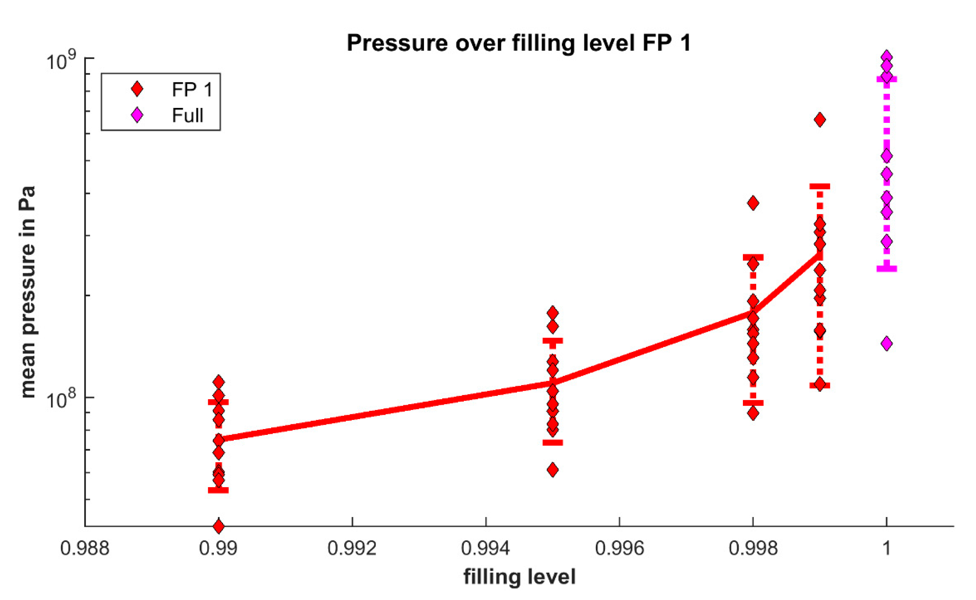
In the logarithmic scale of Figure 10 the approximately linear increase of the curves in the equidistant range between 0.95 and 0.99 illustrates the exponential increase in the mean pressure for increasing filling levels. This increase is particularly pronounced between 0.99 and 1. This is shown as an example with FP 1 in Figure 11 in which a closer look at the regime near the full filling is shown.
It is clearly visible that the pressure drop is very sharp. If the filling level is reduced by 1% (from 1.0 to 0.99) the pressure is reduced by 90%. When decreasing the filling level by 1‰ (from 1 to 0.999) the mean pressure drops from to . That corresponds to halving of the mean pressure. As will be explained in the discussion section, this effect is essential when evaluating partially filled gaps.
4. Summary, Discussion and Outlook
This study aimed to examine the validity of two fundamental assumptions in micro-EHD simulations. These two assumptions on the macroscopic scale are a hydrodynamic pressure of zero in regions where the gap is not completely filled and an independence of the shear flow factor from the filling degree θ. For this purpose, studies were carried out on a microscopic scale.
With the authors PFG model, it is possible to investigate how large the shear flow factors and the average pressures in the gap are when the gap is partially filled. In this context, full filling is a special case of this model, which serves as a reference to many studies in the literature. It was shown that the PFG model provides comparable results to the shear flow factors determined by different methods in the literature.
The PFG model also allows arbitrary distribution of the fluid. This is particularly helpful because the actual fluid distribution on the microscopic scale can hardly be reliably determined when the system is partially filled. For this reason, different fluid distributions were implemented here. This strategy was aimed at limiting the uncertainty resulting from the actual and unknown fluid distribution. Extreme scenarios were used in which particularly large or small areas are completely filled. This methodology allows to specify a certain range for the influence of the partial filling.
It was shown that not only the total amount of fluid in the gap is a decisive parameter, but also how large the partial area in the domain is that is fully filled—the more cells are fully filled, the higher the shear flow factor and the mean pressure is. The variance of the topographies regarding their roughness is significant for the pressure and the fluid flow. The topography roughness variance was in the range of 10% and comparable to the resulting variance of the shear flow factors (in the range of 13% to 17%). In contrast to this, the variance of the pressure was in the range of 56% at the fully filled scenario that characterizes the high nonlinearity near this regime. When decreasing the filling level, the pressure and the flow drops sharply. This behavior is expected and as shown in the introduction, a not fully filled state is often regarded as cavitation region.
However, the results near the fully filled regions must be treated carefully as the transition from a fully filled (pressure) region to a cavitation regime is more complex than commonly assumed. In this context, for the regimes that are close to the fully filled state, the impact of partially filled domains can be significant.
The results imply that the physical pressure buildup in a partially filled domain is substantially different from a fully filled domain. The flow decreases stronger than commonly assumed with decreasing filling level as the microscopic Poiseuille flow term contributes disproportionately less flow. Additionally, the decrease in hydrodynamic pressure buildup consequently leads to a higher portion of the load being transmitted by solid body contacts. With regard to the current conventional treatment of micro-EHD according to the two fundamental assumptions, it is concluded that for the parameter sets used here neglecting the pressure buildup is a valid approach for partially filled gaps with a filling level of roughly 0.9 and less, because less than 1% of the fully filled pressure occurs. For partially filled gaps with a filling level above 0.9 the pressure buildup should be taken into account. Especially very close to full filling, larger discrepancies to reality could occur, since the assumption of a pressure of zero can cause significant deviations here.
For calculating the shear flow factor and the shear stress the partially filled domains should be considered. In contrast to the current conventional implementation, the shear flow factor is dependent on the filling level—in the studies performed in this study it is halved from filling level 1 to 0.95 (from mean value of −0.518 at full filling to a mean over all filling procedures of −0.259 at 0.95). The different filling procedures showed that the pressure buildup and the shear flow factor significantly depend on the transient fluid distribution in the gap (difference between the mean value of the filling procedure ranges from −0.201 for FP1 to −0.370 for FP3 at 0.95 filling).
The conclusions reached here are based on an exemplary study, which did not claim to formulate a general solution with all relevant dependencies but should rather serve to draw attention to the problem and suggest possible solutions. For a fundamental solution further comprehensive studies are necessary, which would also require a greater variation of topographies and mean gap heights.
The authors are aware that the partially filled areas of a gap are not as important for the system behavior and the overall dynamics as the areas with fully filled gaps. Thus, the influence of the shear flow factors in the cavitation area is certainly not as large as in the convergent (fully filled) gap, but for the shear stresses and the resulting resistance the effect can still become significant. Furthermore, with this consideration, the local transition between fully filled and partially filled gaps can be described more precisely, also especially for the pressures.
All effects presented in this paper depend on the actual fluid distribution in the gap. This information however is not easily available and depends on the transient flow in the rough gap. First simulations of this problem were completed with the PFG model and will also be the subject of further investigations in the future.
Author Contributions
Conceptualization, M.M. and G.-P.O.; data curation, L.S.; formal analysis, L.S.; funding acquisition, M.M. and G.-P.O.; investigation, L.S.; methodology, M.M., L.S. and G.-P.O.; project administration, M.M.; software, L.S.; supervision, M.M. and G.-P.O.; validation, L.S.; visualization, L.S.; writing—original draft, L.S.; writing—review & editing, M.M. All authors have read and agreed to the published version of the manuscript.
Funding
This research was funded by “Deutsche Forschungsgemeinschaft (DFG)” project number 390252106 “Grundsatzuntersuchungen zu tribologischen Kontakten mit teilgefüllten Spalten” (Fundamental Studies on Tribological Contacts with partially filled gaps (http://gepris.dfg.de/gepris/projekt/390252106?language=en). We acknowledge support by the German Research Foundation and the Open Access Publication Funds of the Technische Universität Braunschweig.
Acknowledgments
The authors thank Laura Hahn and Yanhong Mi for carrying out numeric studies.
Conflicts of Interest
The authors declare no conflicts of interest.
References
- Reynolds, O. On the theory of lubrication and its application to Mr. Beauchamp tower’s experiments, including an experimental determination of the viscosity of olive oil. Philos. Trans. R. Soc. Lond. 1886, 177, 157–234. [Google Scholar] [CrossRef]
- Dowson, D.; Higginson, G.R. A Numerical Solution to the Elasto-Hydrodynamic Problem. J. Mech. Eng. Sci. 1959, 1, 6–15. [Google Scholar] [CrossRef]
- Liu, Y.; Wang, Q.J.; Bair, S.; Vergne, P. A Quantitative Solution for the Full Shear-Thinning EHL Point Contact Problem Including Traction. Tribol. Lett. 2007, 28, 171–181. [Google Scholar] [CrossRef]
- Elrod, H.G.; Adams, M.L. A Computer Program for Cavitation and Starvation Problems. In Proceedings of the 1st Leeds-Lyon Symposium on Tribology, Leeds, UK, 6–9 September 1974; pp. 37–41. [Google Scholar]
- Patir, N.; Cheng, H.S. An Average Flow Model for Determining Effects of Three-Dimensional Roughness on Partial Hydrodynamic Lubrication. J. Lub. Tech. 1978, 100, 12. [Google Scholar] [CrossRef]
- Müller, M.; Ostermeyer, G.-P.; Bubser, F. A contribution to the modeling of tribological processes under starved lubrication. Tribol. Int. 2013, 64, 135–147. [Google Scholar] [CrossRef]
- Müller, M.; Stahl, L.; Ostermeyer, G.-P. Experimental Studies of Lubricant Flow and Friction in Partially Filled Gaps. Lubricants 2018, 6, 110. [Google Scholar] [CrossRef] [Green Version]
- Etsion, I.; Pinkus, O. Solutions of Finite Journal Bearings With Incomplete Films. J. Lub. Tech. 1975, 97, 89. [Google Scholar] [CrossRef]
- Etsion, I.; Barkon, I. Analysis of a Hydrodynamic Thrust Bearing With Incomplete Film. J. Lub. Tech. 1981, 103, 355. [Google Scholar] [CrossRef]
- Tanaka, M. Journal bearing performance under starved lubrication. Tribol. Int. 2000, 33, 259–264. [Google Scholar] [CrossRef]
- Wang, W.-Z.; Li, S.; Shen, D.; Zhang, S.; Hu, Y.-Z. A mixed lubrication model with consideration of starvation and interasperity cavitations. Proc. Inst. Mech. Eng. Part J J. Eng. Tribol. 2012, 226, 1023–1038. [Google Scholar] [CrossRef]
- Dowson, D.; Taylor, C.M. Cavitation in bearings. Annu. Rev. Fluid Mech. 1979, 11, 35–65. [Google Scholar] [CrossRef]
- Ausas, R.; Ragot, P.; Leiva, J.; Jai, M.; Bayada, G.; Buscaglia, G.C. The Impact of the Cavitation Model in the Analysis of Microtextured Lubricated Journal Bearings. J. Tribol. 2007, 129, 868–875. [Google Scholar] [CrossRef]
- Bayada, G.; Martin, S.; Vázquez, C. An Average Flow Model of the Reynolds Roughness Including a Mass-Flow Preserving Cavitation Model. J. Tribol. 2005, 127, 793–802. [Google Scholar] [CrossRef] [Green Version]
- Sahlin, F.; Almqvist, A.; Larsson, R.; Glavatskih, S. A cavitation algorithm for arbitrary lubricant compressibility. Tribol. Int. 2007, 40, 1294–1300. [Google Scholar] [CrossRef]
- Patir, N.; Cheng, H.S. Application of Average Flow Model to Lubrication Between Rough Sliding Surfaces. J. Lub. Tech. 1979, 101, 220. [Google Scholar] [CrossRef]
- Müller, M.; Jäschke, H.; Bubser, F.; Ostermeyer, G.-P. Simulative studies of tribological interfaces with partially filled gaps. Tribol. Int. 2014, 78, 195–209. [Google Scholar] [CrossRef]
- Müller, M.; Völpel, A.; Ostermeyer, G.-P. On the influence of fluid dynamics and elastic deformations on pressure buildup in partially filled gaps. Tribol. Int. 2017, 105, 345–359. [Google Scholar] [CrossRef]
- Tripp, J.H. Surface roughness effects in hydrodynamic lubrication: the flow factor method. J. Lub. Tech. 1983, 105, 458–463. [Google Scholar] [CrossRef] [Green Version]
- Rienäcker, A. Instationäre Elastohydrodynamik von Gleitlagern mit Rauhen Oberflächen und Inverse Bestimmung der Warmkonturen; Universität Kassel: Kassel, Germany, 1995. [Google Scholar]
- Bartel, D. Simulation von Tribosystemen. Grundlagen und Anwendungen; Vieweg+Teubner: Wiesbaden, Germany, 2010; ISBN 978-3-8348-9656-8. [Google Scholar]
- Shen, C.; Khonsari, M.M. On the Magnitude of Cavitation Pressure of Steady-State Lubrication. Tribol. Lett. 2013, 51, 153–160. [Google Scholar] [CrossRef]
- Shen, C.; Khonsari, M.M. Effect of Dimple’s Internal Structure on Hydrodynamic Lubrication. Tribol. Lett. 2013, 52, 415–430. [Google Scholar] [CrossRef]
Figure 1.
Mechanical contact with a partially filled gap.

Figure 2.
Experimental results of studies performed on the Wear Debris Investigator (WDI) [7]. (a) Coefficient of friction over total fluid volume; (b) fluid distribution for varying rotational speeds and viscosities.
Figure 2.
Experimental results of studies performed on the Wear Debris Investigator (WDI) [7]. (a) Coefficient of friction over total fluid volume; (b) fluid distribution for varying rotational speeds and viscosities.
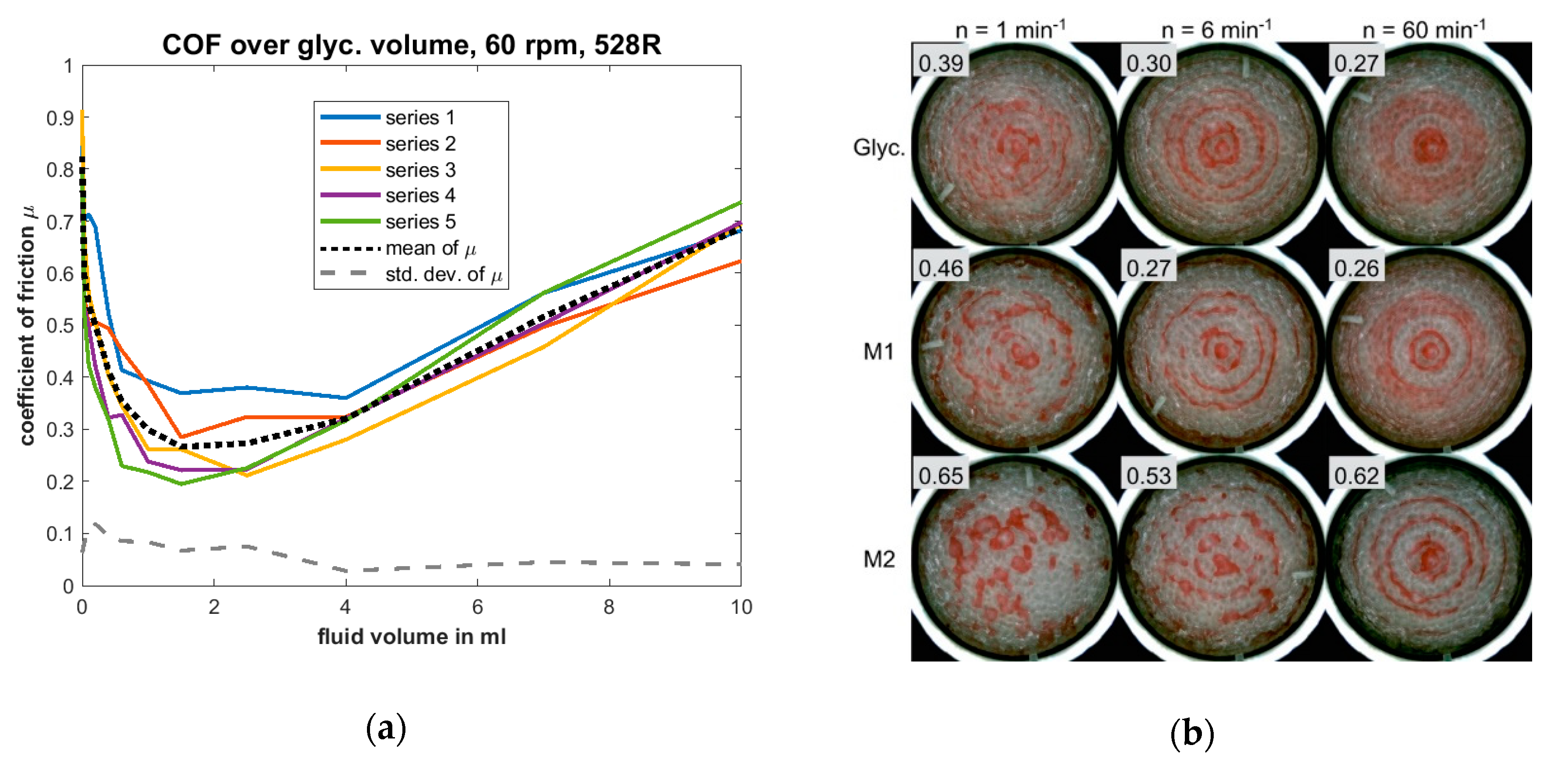
Figure 3.
Basic idea of the partially filled gaps (PFG) model [6].
Figure 3.
Basic idea of the partially filled gaps (PFG) model [6].
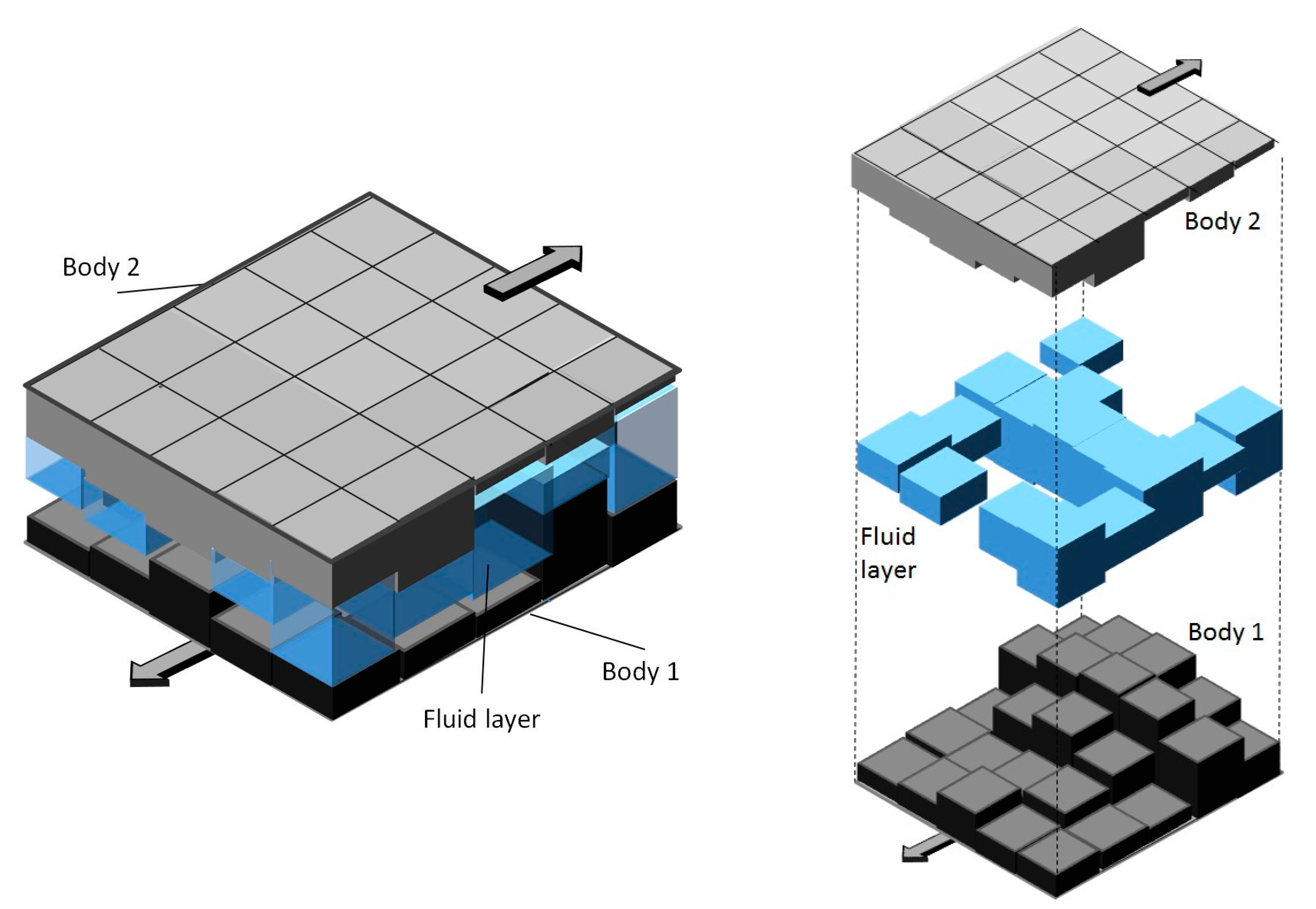
Figure 4.
Constitutive laws and their interaction within the PFG model [17].
Figure 4.
Constitutive laws and their interaction within the PFG model [17].
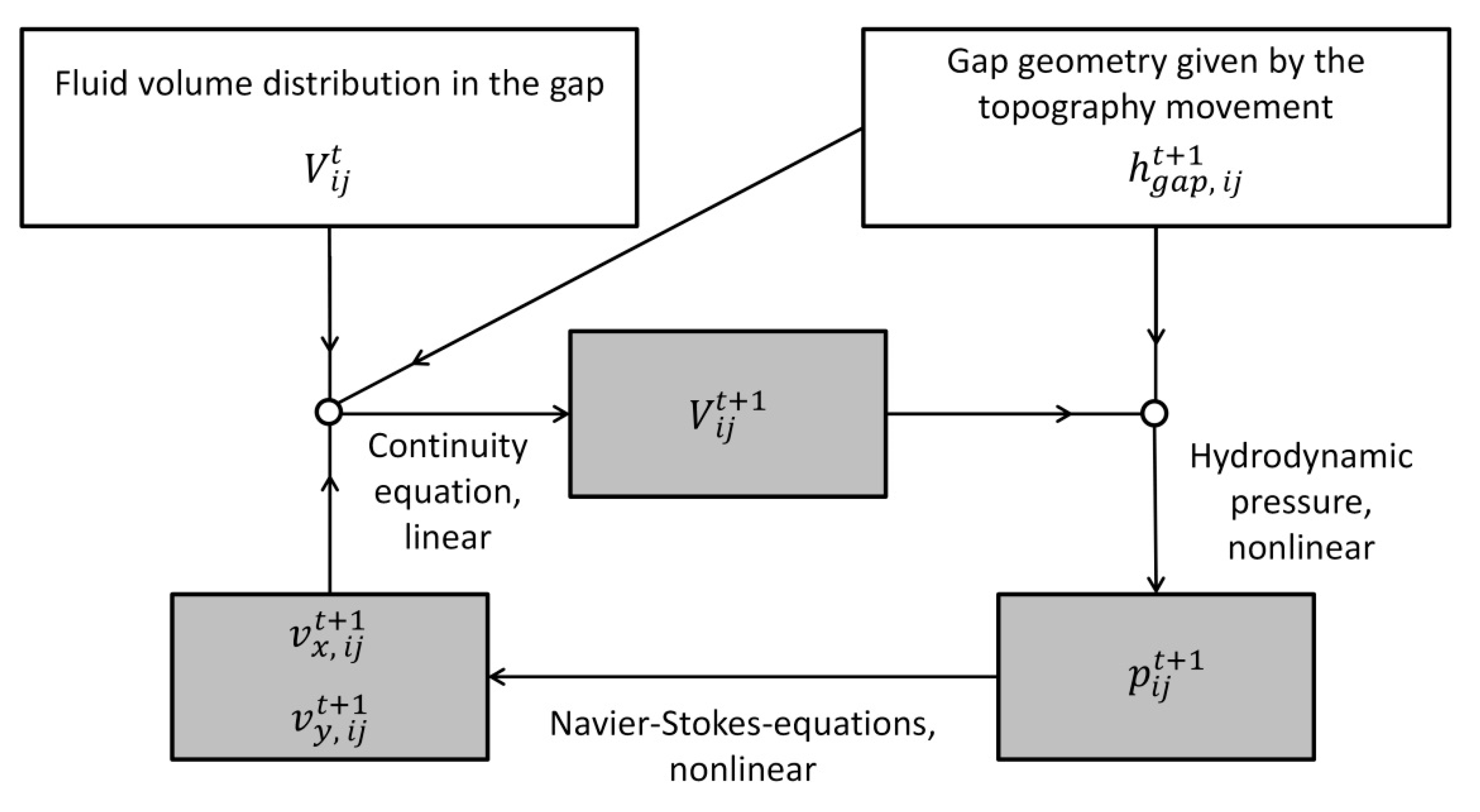
Figure 5.
Shear flow factors for fully filled gaps over , calculated with the PFG model and compared to other established approaches with Peklenik factor of 1.
Figure 5.
Shear flow factors for fully filled gaps over , calculated with the PFG model and compared to other established approaches with Peklenik factor of 1.
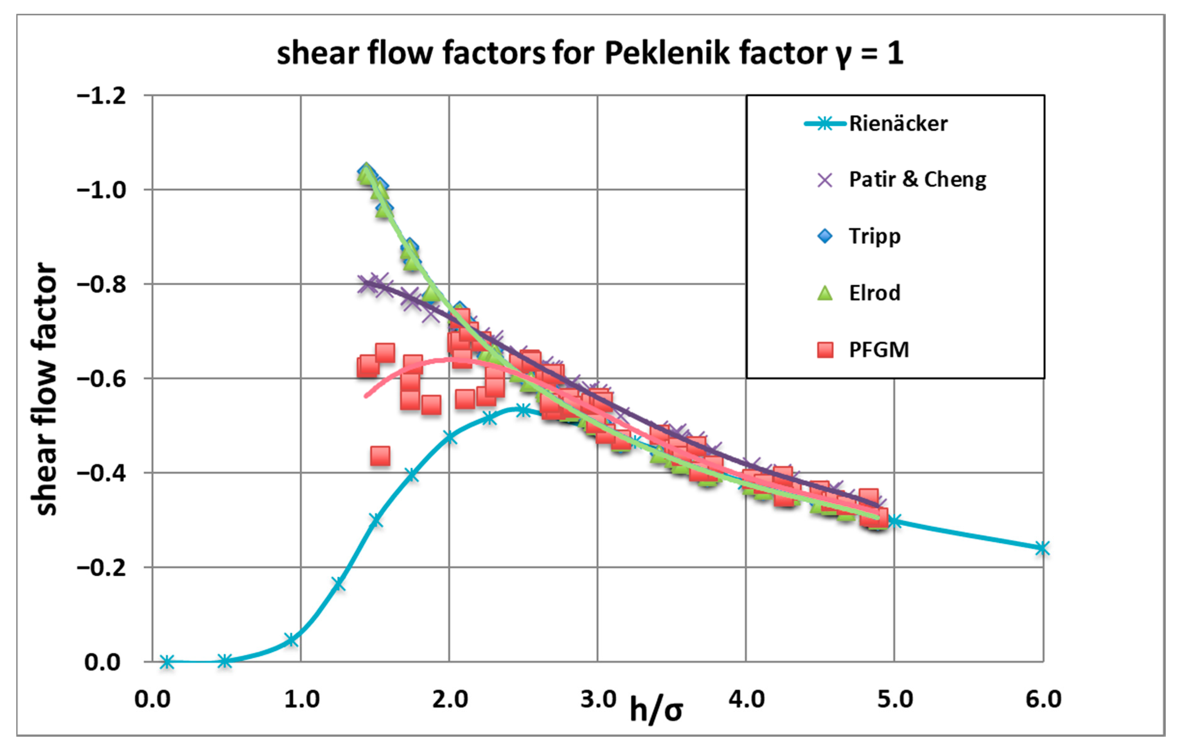
Figure 6.
Variance of surface topographies.
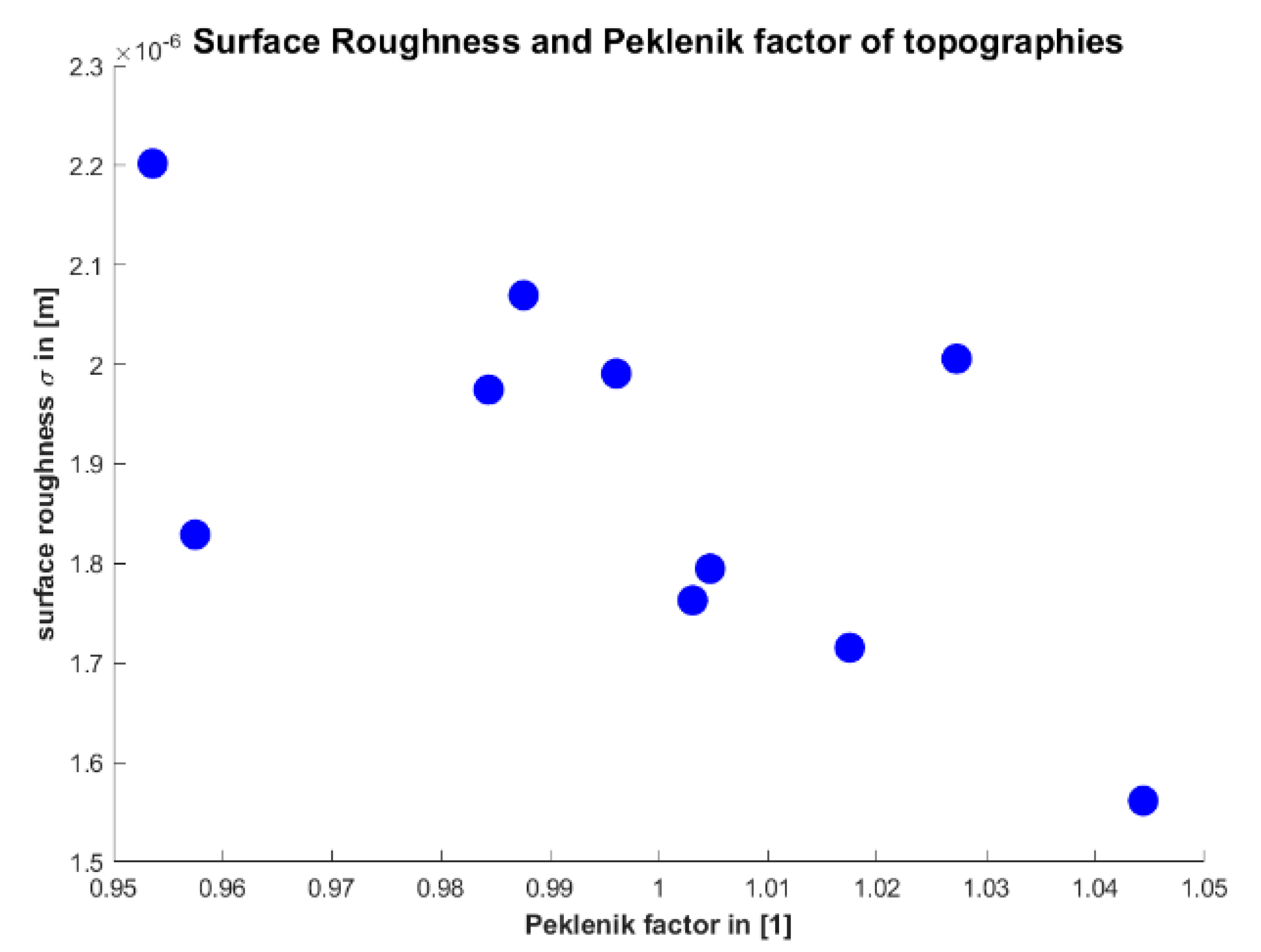
Figure 7.
Gap height of topography “3”.

Figure 8.
Shear flow factor over the filling level and filling procedures.

Figure 9.
Ratio of fully filled cells to total number of cells over the filling level for topography “5”.
Figure 9.
Ratio of fully filled cells to total number of cells over the filling level for topography “5”.

Figure 10.
Mean pressure over the filling level and filling.
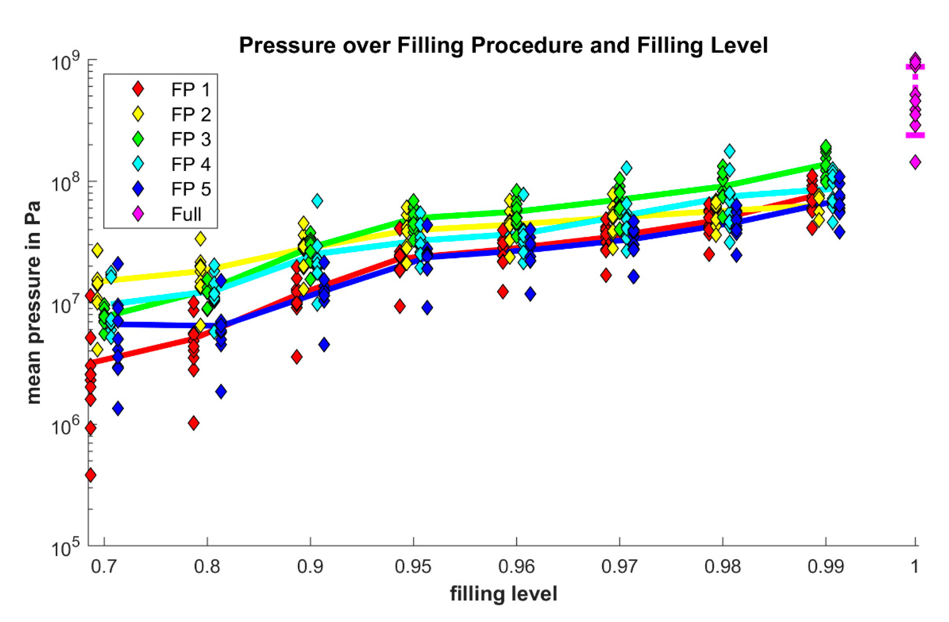
Figure 11.
Mean pressure near fully filled regime for filling procedure (FP) 1.

Table 1.
Illustrations and explanations for the filling procedures.
FP1: “filling level”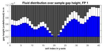 | This procedure applies the filling level to each individual cell. Thus, no cell is initially fully filled, but each cell is partially filled with the same filling level. This procedure corresponds to a state in which initially no cell is fully filled, and no fluid pressure is present. With the movement of the topographies the fluid flows and full cells appear. |
FP 2: “bottom up”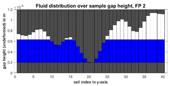 | This procedure fills the gap metaphorically from the bottom up. The fluid is distributed so that the absolute fluid volume in each cell is the same. If a cell is smaller than that volume, the cell is fully filled with its respective fluid volume. This leads to homogenous distribution of fluid in the gap and the number of initially fully filled cells is small. |
FP 3: “big to small” | This procedure fills the gap starting with the cell of greatest gap height. Subsequently, the second greatest cell is filled. This procedure continues until the available fluid volume (according to the filling level) is distributed. The cell that is filled last may only be partially filled (here cell 4). This leads to an inhomogeneous distribution with a relatively large number of fully filled cells. |
FP 4: “random cells”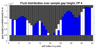 | This procedure fully fills random cells. A random cell is selected and fully filled until the available fluid volume is distributed (according to global filling level). The cell that is filled last may only be partially filled (here cell 24). This procedure leads to a distribution with a large number of fully filled cells. |
FP 5: “random”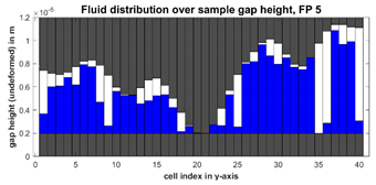 | This procedure chooses a random cell and attempts to fill it with a random amount of fluid. If the chosen amount fits into the cell (cell empty or only partially filled), the procedure fills it and proceeds. If the chosen amount does not fit into the remaining volume in the chosen cell, the procedure continues with a new random cell and a new random amount of fluid. The procedure continues until the complete fluid volume is distributed. Each cell can be chosen multiple times. This leads to a situation where most cells has a high filling level, but none is completely filled. |
© 2020 by the authors. Licensee MDPI, Basel, Switzerland. This article is an open access article distributed under the terms and conditions of the Creative Commons Attribution (CC BY) license (http://creativecommons.org/licenses/by/4.0/).
Share and Cite
MDPI and ACS Style
Müller, M.; Stahl, L.; Ostermeyer, G.-P. Studies on the Pressure Buildup and Shear Flow Factors in the Cavitation Regime. Lubricants 2020, 8, 82. https://doi.org/10.3390/lubricants8080082
AMA Style
Müller M, Stahl L, Ostermeyer G-P. Studies on the Pressure Buildup and Shear Flow Factors in the Cavitation Regime. Lubricants. 2020; 8(8):82. https://doi.org/10.3390/lubricants8080082
Chicago/Turabian StyleMüller, Michael, Lukas Stahl, and Georg-Peter Ostermeyer. 2020. "Studies on the Pressure Buildup and Shear Flow Factors in the Cavitation Regime" Lubricants 8, no. 8: 82. https://doi.org/10.3390/lubricants8080082
Note that from the first issue of 2016, this journal uses article numbers instead of page numbers. See further details here.