Life Satisfaction: Insights from the World Values Survey

Homocianu, Daniel

doi:10.3390/soc14070119

Open AccessArticle

Life Satisfaction: Insights from the World Values Survey

by

Daniel Homocianu

Department of Accounting, Business Information Systems, and Statistics, Faculty of Economics and Business Administration, Alexandru Ioan Cuza University, 700505 Jassy, Romania

Societies 2024, 14(7), 119; https://doi.org/10.3390/soc14070119

Submission received: 2 April 2024 / Revised: 19 June 2024 / Accepted: 8 July 2024 / Published: 15 July 2024

(This article belongs to the Special Issue Healthy Lifestyle: The Relevance of Health Promotion for Society)

Download

Browse Figures

Review Reports Versions Notes

Abstract

:

This paper explores enduring influences on life satisfaction using empirical analysis of World Values Survey (WVS) data (four versions of the most comprehensive dataset, namely 1.6, 2.0, 3.0 and 4.0). Five significant values emerged—financial satisfaction, happiness, freedom of choice, health, and democracy. Through rigorous selection processes and various statistical techniques, a subset of three determinants resulted, along with consecrated socio-demographic variables such as age, gender, marital status, social class, and settlement size. Advanced methodologies such as feature selection, random and non-random cross-validations, overfitting removal, collinearity and reverse causality checks, and different regressions served to evaluate and validate robust models. Nomograms helped to predict life satisfaction probabilities. The findings contribute to understanding life satisfaction dynamics and offer practical insights for future research and policy.

Keywords:

life satisfaction; feature selection; cross-validation; overfitting; collinearity; reverse causality; regression and classification models

1. Introduction

Life satisfaction seems to be a complex and subjective concept that can vary greatly from person to person and can depend on many factors such as personal values, relationships, health, financial situation and stability, and life experiences. As evidence of its subjective specificity, the related concept of “subjective well-being” was also considered and discussed as most dependent on perspective [1], the relationship between the desired and the real [2], and, ultimately, cultural differences [3] and how individuals understand concepts such as life meaning and subjective well-being [4]. While some people find happiness in money [5] and material possessions [6,7,8], others find it in spiritual or emotional fulfillment [9]. Life satisfaction does not seem to be under the governance of a single formula. Moreover, its attainment varies from person to person, and individuals must discern what brings them fulfillment and happiness and actively pursue those aspects in their personal lives. There could also be general and specific patterns for this satisfaction. As for the first category, a consistent amount of high levels of life satisfaction is reported (a share of almost 70%) as resulting from the answers of respondents from 108 countries in the latest version (v.4.0) of the most comprehensive dataset from the World Values Survey, covering almost the entire period from 1981 to 2022.

The study of life satisfaction is not something new. Historically, this research line can be rooted in the 18th century [10], associated with Enlightenment thought. From this point of view, the purpose of existence is life itself rather than serving the ruler or God. Therefore, self-improvement and happiness become central values in a society responsible for providing citizens with what is necessary for a good life. The same conviction manifested a century later in the form of the Utilitarian Creed that the best society is that which offers the greatest happiness for the highest number of people and inspired large-scale attempts to carry out social reform and influenced the development of the welfare state two centuries later [11,12]. The overall progress started with creative efforts to build a better society, translated first into attempts to avoid ignorance, disease, hunger, and poverty, as well as increasing the level of literacy and controlling diseases and epidemics, and later into ways to ensure a good life for all, and a good material standard of living through monetary earnings, income security, and income equality. The latter has given rise to much social research on poverty and social inequality [13,14]. Later, the term quality of life emerged in the context of new themes related to the limits to economic growth and post-materialism.

Regarding differences between life satisfaction and happiness [15], the latter is often described as a more momentary and emotional state [16,17,18,19], often influenced by external factors such as events, experiences, or possessions. It can be short-lived and fluctuate frequently. On the other hand, life satisfaction is a more enduring and cognitive evaluation of a particular life as a whole (overall happiness) [20,21,22,23]. It encompasses many factors, including an individual’s overall sense of purpose, relationships, financial stability, health, etc. Life satisfaction tends to be a more stable and long-term assessment of happiness. It is worth noting that while there is often an overlap between happiness and life satisfaction, they are not the same thing and can exist independently of each other. One can feel happy at a particular moment but still have low life satisfaction or vice versa.

Moreover, life satisfaction, as a key component of well-being, can be categorized into eudaimonic well-being, which emphasizes meaning, self-realization, or excellence, and hedonic well-being, which focuses on pleasure and the avoidance of pain [24]. In addition, the Cybernetic Value Fulfillment Theory posits that well-being is the fulfillment of psychologically integrated, nonconflicting values unique to each individual [25].

Other studies also indicate the role of socio-demographic and individual features [26,27,28]. They emphasize influences from this category, such as age, gender [29], psychological features, lifestyle, participation in leisure activity, and satisfaction related to spending free time or leisure satisfaction [30].

The disciplinary perspectives that this article takes can be identified as:

A-Social Sciences (Psychology and Sociology): (1) Focus on life satisfaction as a psychological construct; (2) Analysis of values such as happiness, freedom of choice, health, and democracy as determinants of life satisfaction; (3) Use of World Values Survey (WVS) data to explore enduring influences on life satisfaction; (4) Incorporation of socio-demographic variables (age, gender, marital status, social class, settlement size) to understand variations in life satisfaction; (5) Contribution to understanding life satisfaction dynamics from a sociological perspective.

B-Economics: (1) Examination of financial satisfaction as a key determinant of life satisfaction; (2) Economic analysis of the impact of financial well-being on overall life satisfaction; (3) Statistical techniques and advanced methodologies (feature selection, regressions, nomograms) used to model and predict life satisfaction probabilities; (4) Practical insights for economic policy based on empirical findings.

C-Statistics and Data Science: (1) Application of advanced statistical techniques (feature selection, random and non-random cross-validation, overfitting removal, collinearity checks, reverse causality checks) to analyze World Values Survey data; (2) Utilization of different regression models to evaluate and validate robust models of life satisfaction; (3) Nomograms as a tool for visualizing and predicting life satisfaction probabilities; (4) Emphasis on rigorous data analysis and methodological approaches in social sciences research.

D-Policy and Governance: (1) Practical implications for policymaking based on insights into determinants of life satisfaction; (2) Implications for democratic governance and social policies related to happiness, freedom of choice, and health; (3) Contribution to evidence-based policy decisions regarding socio-demographic factors affecting life satisfaction.

These disciplinary perspectives collectively highlight the multidimensional approach taken in this article to understand life satisfaction dynamics, combining insights from psychology, sociology, economics, statistics, data science, and policy and governance implications.

The article further reviews the literature on the perceptions related to life satisfaction. Then, it describes the data and methodology used before presenting and discussing the main findings in a dedicated section. The latter captures the focus of the current study, namely the discovery of the most resilient influences related to life satisfaction, and this is achieved by eliminating redundancies after performing many robustness checks in advance.

2. Related Work

Life satisfaction is more liable to shifts in aspiration level [31] when compared to happiness, thus reducing the comparability of the resulting indices. Moreover, life satisfaction is the evaluation of personal life as a whole, not simply the current level of happiness [32].

Among other scholars, refs. [33,34] emphasized that health is usually significantly correlated with life satisfaction. According to some other authors [35,36], higher levels of freedom of choice and control are usually strongly associated with life satisfaction.

From other perspectives [37,38], those with higher levels of financial satisfaction are also more inclined to show higher levels of life satisfaction.

According to other scholars, those more inclined and exposed to democracy as an expression of the will of the people [39] and also of the subjectivity of society [40] or as a crucial way to realize human rights [41], are also more likely to be satisfied with their lives [42,43].

The consecrated socio-demographic features [44] are also significant influences associated with this type of satisfaction. For instance, some researchers [45,46,47,48,49] invoke the U-shape when it comes to the graphical representation of the influence of age on life satisfaction, with high levels of life satisfaction in young adulthood, a gradual decline in middle age with a minimum of being satisfied with life between 40 and 60 years of age, and then an increase in later life. Other studies [50] have found a more complex relationship between age and life satisfaction, with multiple peaks and valleys throughout life. Concerning the relation between gender and this type of satisfaction, it seems the latter also depends on the stability or transitions in marital status [51]. Other studies revealed significant correlations between personality, self-esteem, and life satisfaction [52] or between optimism-related variables, goal orientation, and the same type of satisfaction [53].

A salient and succinct point from this literature review is that life satisfaction is determined by multiple factors, including happiness, health, autonomy, economic contentment, democracy, and democratic values, Big Five personality traits, and socio-demographic characteristics, with significant correlations observed between these variables and overall life satisfaction.

Consequently, the main hypotheses of this paper are:

H1 .

Happiness is closely related to life satisfaction, even if it is far from acting as synonymous with it [54].

H2 .

Good health [55] and freedom of choice and control [56,57] are strongly related to well-being, happiness, and this type of satisfaction [58].

H3 .

Financial choice and satisfaction are closely associated with well-being, the latter being considered more than just happiness and life satisfaction [59]. Therefore, the first two are also related to being satisfied with life.

H4 .

Democratic values [60] positively correlate with increased life satisfaction.

H5 .

Some of the consecrated socio-demographic factors may also predict life satisfaction [61,62,63].

In terms of identified research gaps, most of the existing quantitative studies use data limited in terms of time (a questionnaire at a precise moment in time, a questionnaire applied within a given period/wave) or space (only one country or continent, or at most comparisons between several countries or between a limited number of regions). Moreover, most of the existing papers do not have the stated purpose of identifying the core intersecting predictors of life satisfaction starting from a dataset so varied in time, space, and consecrated socio-demographic features of respondents. Added to this is the fact that most studies do not use simultaneous cross-validation according to random (10-fold) and non-random criteria (both socio-economic criteria and different versions of the dataset).

3. Materials and Methods

This article started from one of the most comprehensive World Values Survey (WVS) datasets. The latter (version 4.0, WVS_TimeSeries_4_0.dta) includes 1045 variables and 450,869 raw observations. It served all selection rounds. Three other versions have been used just in the first selection round (Adaptive Boosting in Rattle), namely: version 3.0 (WVS_TimeSeries_1981_2022_Stata_v3_0.dta, 1,041 variables and 440,055 observations, available online on the WVS site until the end of 2022), version 2.0 (WVS_TimeSeries_1981_2020_stata_v2_0.dta, 1072 variables, and 432,482 records) and 1.6 (WVS_TimeSeries_stata_v1_6.dta, 1045 variables, and 426,452 observations), the latter two still available on the WVS site, namely https://www.worldvaluessurvey.org [accessed on 9 January 2023]. Their .csv exports1 were preceded by designing, testing, and running a script sequence2 responsible for removing the DK/NA [64] values (Do not Know/No Answer/Not Applicable coded by WVS as negative ones, artificially increasing the scales, and not beneficial for selections, Figure 1 and Listing A1, Appendix A) of all variables and also by a simple binary derivation3 (A170bin) of the original variable to analyze (A170, Satisfaction with your life). And this applies considering the two symmetric halves of its original scale (1–5 for 0, and 6–10 for 1, Listing A2, Appendix A). Moreover, the option to generate numerical values for labeled variables (instead of the text) was enabled when exporting (e.g., export delimited using “F:\data\WVS-TS4_A170bin.csv”, nolabel replace). Figure 1 visually depicts the frequency counts of variables, including the target variable A170 (life satisfaction), before and after correcting an artificial scale increase caused by initially encoding “Don’t Know” (DK) or “Not Applicable” (NA) responses as negative numbers in the dataset. This correction process is applied uniformly across all variables, illustrating how it impacts the distribution patterns and ensuring that subsequent analyses are based on accurately scaled data. The figure plays a critical role in demonstrating the methodological step taken to enhance the reliability and validity of analyses related to life satisfaction and other variables in the dataset.

The next step was to load these .csv exports into the Rattle interface (version 5.5.1—started using two commands in R, namely library(rattle) and rattle()), then set A170bin as the target, ignore its source (A170) from the list of inputs, and apply the Adaptive Boosting technique for the decision tree classifiers [65]. This step ran [66,67] for four versions of this most comprehensive dataset of WVS (v4.0, 3.0, 2.0, and 1.6) using default settings (online available at https://tinyurl.com/2wrd3ju6 [accessed on 19 June 2024]). The purpose was to discover the most resilient related variables at the intersection of those four versions (cross-validation considerations). The latter was the 1st selection round (9 resulting variables—Figure 2).

Other alternative selections applied only to the most recent and comprehensive version (4.0) and starting after the same DK/NA treatments considered:

(a): The use of the Naïve Bayes classification algorithm inside the Microsoft DM add-in for spreadsheets (Figure 3) that works together with SQL Server Analysis Services 2016 (as model persistence layer) in a Windows 10 Professional X64 virtual machine (VM—Oracle Virtual Box) configured with 16 GB of RAM of those 32 of the physical machine (Windows 8.1 Professional X64 used for Adaptive Boosting) and two physical cores of those four (Intel Core I7 4710HQ CPU);
(b): The use of filter options applied to the results of a correlation command (PCDM) for selections in Stata 17 (invoked for both forms of the target variable, namely A170 and A170bin, Figure 4) inside the same VM. First, they meant a minimum threshold of 0.1 [68] for the absolute values of pairwise correlation coefficients [69] between each recoded variable from the previous step and the one to analyze. In addition, a maximum accepted p-value (max p = 0.001) and a minimum support afferent to a minimum number of valid observations for the target variable (at least half the total corresponding number—444,917/2, Figure 4) for each pair.

Only seven (7) variables proved to be the most resilient at the intersection of Adaptive Boosting (Rattle in R), Naïve Bayes (Analysis Services), and PCDM (Stata). These are A008, A009, A173, C006, E235, E236, and X047_WVS. From these seven, only the first six were confirmed (successive invocations until no loss in selection) when using CVLASSO (for performing random cross-validation) and RLASSO (for removing overfitting) available after installing the LASSO package [70], and the BMA (Bayesian Model Averaging) command in Stata 17 for both forms of the target variable (S002VS set as an auxiliary influence in BMA).

Additionally, some consecrated socio-demographic variables served non-random cross-validation and later as control. For the first (non-random cross-validation), these variables helped mixed-effects models [71,72,73] in Stata 17 MP (64-bit version). Such models included both fixed effects (the remaining six variables after the previous selection phases) and random ones (clusters on gender, age, marital status, number of children, education level, income level, professional situation, settlement size, country, and survey year, all as socio-demographic variables, bottom of Table A1, Appendix A).

The immediate selection phase measured the existing collinearity between the remaining influences (those six above). First, a matrix with correlation coefficients augmented with intensity bars has been generated only for these six remaining influences [68]. In addition, ordinary least squares (OLS) regressions served the same purpose by measuring the computed VIF (Variance Inflation Factor) against (Equation (1)) the maximum accepted VIF threshold of the model [74,75] for all combinations of two influences of those 6 (combinations of n = 6 taken by k = 2, meaning 15 possibilities—Equation (2)). E235 and E236 emerged as being collinear at this point.

Model’s maximum accepted VIF = 1/(1 − model’s R-squared)

(1)

C(n,k) = n!/(k!(n − k)!)

(2)

where: C(n,k) is the number of combinations of n taken by k;

n! is “n—factorial” or 1 × 2 × … × n;
k! is “k—factorial” or 1 × 2 × … × k;
(n − k)! is “(n − k)—factorial” or 1 × 2 × … × (n − k).

In addition, to choose between these two, logistic regressions have been used. The variable that is responsible for generating models with more explanatory power/larger R-squared [76] and more information gain/smaller values for both AIC and BIC [77] was preserved (e.g., E236).

Additionally, two prediction nomograms [78] resulted (one simple and another one augmented with additional details to become self-explanatory) when using the nomolog command (after its previous installation using a specific installation syntax, namely net install st0391, replace from (http://www.stata-journal.com/software/sj15-2) [accessed on 19 June 2024] and considering the most stalwart remaining influences.

Moreover, each consecrated socio-demographic variable previously used for cross-validation (except S003—country code, which consists of numbers not corresponding to a particular intensity scale) served controlling purposes (new models). The latter meant adding them one by one on top of the existing most robust models (the most resilient influences emerging after the previous selection round or the core models) and separately (one per model).

In addition, for each variable in the core and socio-demographic category above, a two-way graphical representation (scatter chart) was automatically generated by considering each corresponding relationship with the outcome variable (life satisfaction in its scale format tabulated on average by peculiar criteria using the tabstat command in Stata).

Finally, reverse causality checks were performed using ordinal logit (ologit) regressions and the scale form of the target variable corresponding to life satisfaction (A170osc). In each of these regressions that considered only one of the remaining input variables, the latter served both as input and outcome, interchanging these roles with A170osc (regression pairs). A larger R-squared (representing smaller differences between the observed data and the fitted values/theoretical model) and/or a lower AIC and BIC (better fit and smaller information loss) for the resulting models are an indication that each of the remaining variables to further select are more likely to be determinants of A170osc rather than vice versa (determined by it).

The reporting of results mainly benefited from the estout prerequisite package (ssc install estout, replace) with support for both the eststo and esttab commands [79,80], allowing the direct generation of tables (in the console and as external files, respectively) with default performance metrics and some additional ones [81] for well-known statistical models.

A persistent Google Drive online container4 keeps all processing and analysis script sequences together with all intermediary results necessary for this study and demos acting as short tutorials [82] able to capture and show at least the dynamics of some selections and supporting this research. Moreover, due to the unavailability of a preview after sharing, the URL for each script has been altered to allow a one-step download (the specific syntax ending with <<&export=download>>). The latter means that no further confirmation is required.

This paper also relied on several multimedia elements [83,84,85,86]. The latter meant combining text, tables, script sequences, graphs or charts including scatter plots and magnitude lines or bars, video captures, and, in addition, visual synthesis and emphasis methods.

The entire methodology used in this paper also stands on three scientific principles: replicability/reproducibility [87,88], triangulation [89,90], and cross-validation [91,92,93].

4. Results

After performing the first selection step using Adaptive Boosting (in the Rattle library—https://rattle.togaware.com of R) on four versions of the WVS dataset, a set of 10 intersecting variables resulted (Figure 2).

As seen in all four sources (online at https://tinyurl.com/2wrd3ju6) of Figure 2, one way to look at the relevance of the resulting variables is by considering their corresponding frequencies of use in the tree construction behind the Adaptive Boosting technique.

Moreover, this was also the first selection round based on cross-validation considering different (increasing) numbers of observations for those four versions of the source dataset with more and more data and the intersecting set of influences found for them (raw individual results online at https://tinyurl.com/2wrd3ju6 [accessed on 19 June 2024] and synthesis in Figure 2).

The results of applying the first alternative selection based on Naïve Bayes classification in Microsoft DM and Analysis Services on version 4.0 (the most comprehensive one) of the WVS dataset (after removing DK/NA values) was a dependency network (Figure 3). Only eight of those nine influences above (all at the intersection of those four columns in Figure 2, except for D002) are present in this network.

Next, some filters served the selections when performing correlations using the PCDM custom command in Stata [69] on the same WVS dataset (the most recent and comprehensive version, 4.0). For instance, min.abs.correl.coeff. = 0.10, min.N = 222,459 (=round of 444,917/2, where 444,917 is the number of valid observations for the target variable, as seen on the top-right and bottom of Figure 4), and maximum p-value of 0.001. The results (Figure 4) indicate only seven of those nine remaining variables above (all bolded in Figure 2 except for D002—low support, meaning just 26,459 observations as seen in the description of variables and general statistics, Table A1 and Table A2, Appendix A, and S002VS—low correlation coefficients below the threshold value of 0.10).

Figure 3. Dependency network based on Naïve Bayes classification in Microsoft Analysis Services showing all identified influences together with the strongest ones for the WVS dataset, version 4.0. Source: The transition from the mightiest links to all links is available in a short video available at https://tinyurl.com/4vjzdz8p [accessed on 19 June 2024].

The next concern was to start from the same nine robust common influences (Figure 2) and perform random cross-validation (cvlasso), selections based on removing overfitting (rlasso), and BMA selections (which report posterior inclusion probabilities—PIP, preferably as close to 1 as possible), all three5 until convergence (no loss) and considering both forms (binary and scale) of the target variable (A170 and A170bin). Cvlasso used both the lse option (largest lambda for which MSPE or the Mean Squared Prediction Error is within one standard error of the minimal MSPE) and the lopt one (the lambda that minimizes MSPE). After this stage, those seven variables above persisted (all in Figure 2 except for D002 and S002VS).

Figure 4. Results of a selection command (PCDM) based on pairwise correlation and additional filters on magnitude, support, and significance for the WVS dataset, version 4.0 (Stata script at https://drive.google.com/u/0/uc?id=1KNUTR0iYoPzytIF2wr2s2aPE6uz4joLI&export=download [accessed on 19 June 2024]).

Next, three rounds6 of non-random cross-validation run using mixed-effects modeling. For the first such round7, just one variable, namely X047_WVS (scale of incomes) of the remaining seven (the ones bolded in Figure 4) acting as fixed effects lost significance (nine from eleven models/scenarios with A170 set as target). And this was observed because of considering many clustering criteria/random effects (the consecrated socio-demographic variables mentioned in the previous section) and two mixed-effects regression types (both melogit for the binary form of the response variable and meologit for the one having values on a scale). If considering only the remaining six as fixed effects8 (all bolded in Figure 4 except for X047_WVS—2nd round of non-random cross-validation), there was no loss in significance no matter the clustering criteria.

To additionally validate the simultaneous removal of both X047_WVS and S002VS at the previous steps (D002—no longer considered due to its low number of valid observations), an additional set of non-random cross-validation (3rd round of non-random cross-validation) based on both melogit and meologit has been performed (8 fixed effects and other ten clustering variables—Table A3, Appendix A). Those six remaining influences above proved to be robust (in terms of no loss of significance) in this additional round, namely A008, A009, A173, C006, E235, and E236. The other two failed at least in one scenario: X047_WVS when cross-validating using most consecrated socio-demographic variables as cluster criteria except for age (X003) and the number of children (X011) and considering the scale form of the target variable (A170), while S002VS (chronology of EVS-WVS waves) when cross-validating using the highest educational level attained (X025), the country code (S003), and the survey year (S020) as cluster criteria and considering both forms of the target variable (A170bin and A170).

Next, when verifying the existing collinearity using the first method, a matrix with correlation coefficients and a minimum visual augmentation using intensity bars for the remaining six influences emerged (Figure 5—all Pearson correlation coefficients are significant at 0.1‰). The latter (as absolute values) shows no evidence of collinearity if considering 0.1 and 0.39 as the lower and upper limits for weak correlation, while 0 and 0.1 as the ones for negligible correlation [68].

In addition, OLS max.Comput.VIF against OLS max.Accept.VIF (Equation (1)) for models with all six previously tested influences (Figure 5) at once (model 1 in Table A4, Appendix A) and additionally taken each two (models 2–16 in Table A4, Appendix A) in all 15 combinations (Equation (2)) served to discover further evidence of collinearity. The removal decision considered one of the two variables. These are E235 and E236, namely the importance of democracy as own value and democracy as perceived in own country, respectively (model 16 in Table A4, Appendix A, namely the only one for which OLSmaxComputVIF > OLSmaxAcceptVIF) [81].

After performing additional logit regressions, E236 brought higher accuracies (AUC-ROC of 0.8350 and 0.8351) and R-squared values (0.2645 and 0.2649) together with better fit due to lower AIC and BIC values than E235 (AUC-ROC of 0.8340 and 0.8345, R-squared of 0.2624 and 0.2638). And this was recorded when considering the binary form of the target variable (model 3 vs. model 4 for comparable support due to the same number of observations using a filtering condition on the variable dropped, and model 5 vs. 6 for all but different numbers of available responses and no filtering condition—Table A5, Appendix A). In the case of additional ologit regressions, the models keeping E235 and dropping E236 had a better R-squared than those keeping E236 and dropping E235. However, the same did not apply in terms of information gain. Consequently, the balance is inclined towards keeping E236 at the expense of removing E235 (the other democracy-related variable).

As support, 234,223 valid intersecting observations (meaning 51.95% of the total number of records for the entire dataset) corresponding to the last three waves were behind the first core model (model 5, Table A5, Appendix A). And this is because all five most resilient influences and the response variable were considered simultaneously only in these three waves (2005–2009, 2010–2014, and 2017–2022), E236 having no observations9 for the first four. The same happened if removing E236 and preserving E235 with a slight increase in the number of responses (more than 245,000 valid intersecting observations—model 6, Table A5, Appendix A) and a slight decrease in terms of accuracy of classification (AUC-ROC = 0.8345). If removing both E235 and E236 (model 2, Table A5, Appendix A), the support increases to 410,513 non-null intersecting observations (meaning 91.05% from the total number, namely 450,869, and also 92.26% from those 444,917 valid for the target variable) while covering all seven waves and increasing the accuracy of classification (AUC-ROC = 0.8458). Furthermore, the four remaining influences are now fully included in the list of the mightiest links in the Naïve Bayes dependency network (Figure 3).

Next, a simple Stata script design (Listing A3, Appendix A) supports the alignment of the scales to 0 for the target variable and those corresponding to some solid influences on it. Another purpose of the latter was to optimize the following two prediction nomograms (Figure 6, nomolog command in Stata) for better readability. Both are based on binary logistic regressions. The corresponding two models are identical to those numbered 2 and 5 (Table A5, Appendix A) in terms of performance metrics and values of coefficients and errors for the top five influences except for the sign of the first two, namely A008 and A009, due to reversed scales (Listing A3, Appendix A). These serve the visual interpretation of all remaining most potent influences. The first nomogram is simple (meaning the exact way it results after generating it using the nomolog command). It corresponds to a model with five resilient influences, with lower support (51.95% of the total number of observations because of E236osc) but still generating a considerable R² (0.2649) and good accuracy of classification (AUC-ROC of 0.8351). The second one corresponds to a model with only those four most resilient influences and high support (91.05% of the total observations of the WVS dataset, version 4.0), generating an R² of 0.2884 and good accuracy of classification (AUC-ROC of 0.8458). This second nomogram is augmented with metadata about the individual score at the intersection with the X-axis (perpendicular lines drawn next to each possible value of the associated influences), respectively, with suggestions for interpreting the input values, their corresponding scores, and the resulting total score and afferent likelihood, so that the nomogram is self-explanatory. The maximum theoretical probability for the most advantageous combination of variable values (extreme right) in both nomograms is high. It indicates a value of more than 0.95 (95%—middle and bottom of Figure 6). These nomograms also reflect the magnitude of marginal effects (better comparability than with raw coefficients) for the corresponding variables. In addition, they serve to understand the cumulated effect size by considering the amplitude of any scale easily noticeable in these visual representations.

Additional controls (Table A6 and Table A7, Appendix A) obtained by adding consecrated socio-demographic variables one by one to the already validated core models with 4 and 5 influences (Figure 6) successfully demonstrated again the robustness of the latter. Moreover, they confirmed or rejected the role of these additional variables. For instance, some of such variables have dramatically lost their significance (X011, Table A6 and Table A7, Appendix A, model 4; X028, Table A6, Appendix A, model 17), while others just changed the sign when considering those two forms of the target variables (X011, X025, X047_WVS, S02VS, and S020). By contrast, the persistence (both in sign and significance) of X001, X003, X007, X045, and X049 (Table A6 and Table A7, Appendix A) indicated a potential role of gender, age, marital status, social class, and settlement size, respectively, in overall models even if they did not pass the previously described selection stages. In addition to the tests performed by including each of the two robust core models above (Figure 6), the remaining five consecrated socio-demographic influences are tested again, this time separately and considering just one per model (Table A8 and Table A9, Appendix A). Under such circumstances, it is noticeable that only the last three (X007, X045, and X049) persisted, while the first two (X001 and X003) changed their sign, lost significance, or both.

The tabulations by mean supporting the two-way graphical representations between the target variable and each of the core variables (top five in Figure 7 from upper-left to lower-right) and also from the socio-demographic category (last eleven on the bottom-right of Figure 7) are also available.

For the specific case of average life satisfaction (Mean_A170osc) against age (X003), the number of non-null responses was also considered (Count_A170osc_byX003—Figure 8). The purpose of the latter was to assess age limits for outliers in terms of frequency (outside the range between 15 to 90 years, meaning at least hundreds of valid records/observations—Table A10, Appendix A) for this specific case of Mean_A170osc versus X003 (middle-right of Figure 7). The relation between average life satisfaction and age shows a much more pronounced U-shape after removing these low-frequency outliers (Figure 9) than earlier (a somewhat flatter “U”—X003, middle-right of Figure 7).

Final cross-validations10 considered models with seven (the quad-core plus marital status/X007osc, social class/X045osc, and settlement size/X049osc) or eight influences (the penta-core plus the same three above) and a reasonable number of criteria for cross-validations. They refuted the last three influences added to those two cores when considering cross-validation criteria such as gender, employment status, the chronology of waves, country, and survey year in the case of the last two of those three (social class and settlement size) or the number of children in the case of marital status, even though the two overall models with 7 and 8 influences did not show multi-collinearity and recorded significance for all corresponding variables and accuracy and R^2 scores better than the two core models with four and five components that already passed all the cross-validation tests.

After performing some reverse causality checks (Table A11, Appendix A section), only three variables from those five most robust influences (model 5, Table A5, Appendix A section) were confirmed as determinants (A173osc, C006osc, and E236osc). Both a separate binary logistic model and a corresponding prediction nomogram (Figure 10) were generated for this triad of predictors (Stata script at https://tinyurl.com/3zenxed6 [accessed on 19 June 2024]). The performance metrics of this model with only three components indicated an AUC-ROC of 0.814 (lower than that of model 5, Table A5, Appendix A, but still indicating good accuracy of classification) and an R-squared of 0.2205. Moreover, the maximum theoretical probability for the most advantageous combination of those three determinant values (right edge of each line in Figure 10) still indicates a value of more than 95% (18 or the sum of 5.75, 10, and 2.25 on the score axis corresponds to much more than 0.95).

5. Discussion

5.1. Main Findings

The main findings highlight the significant influences on life satisfaction: financial satisfaction, happiness, freedom of choice, health, and democracy, each validated through robust empirical analysis of World Values Survey data and consistent with prior research in the scientific literature.

In terms of magnitude (descending order of scale amplitudes), the first and most important of these five influences corresponds to satisfaction with the household financial situation. It indicates that people who are more satisfied in such terms are more likely to show more contentment with their lives (positive influence or the maximum recoded value of 9 for C006osc—the right side of Figure 6). The latter means that this type of financial satisfaction (household-related) is among the best associated with life satisfaction according to WVS data (complete validation of H3). This finding is in line with the already documented relationship between both financial costs and benefits and their well-being implications, as mentioned in the scientific literature [94,95,96,97].

The second most important influence (considering the same magnitude criterion) seems to correspond to the feeling of happiness. The latter belongs to a peculiar variable sub-category defined as <<Important in Life>>. As expected, this shows that those who reported a higher level of happiness are also more likely (positive influence or the maximum recoded value of 3 for A008osc—the right side of Figure 6 and Figure 7) to be satisfied with their lives (complete validation of H1). Although this finding seems close to being obvious, the relationship between happiness and life satisfaction is reciprocal and well-studied [98,99,100].

The third most potent influence found is related to the level of freedom of choice and control. It means that people with a higher level of this type of freedom are also more likely (positive influence or the maximum recoded value of 9 for A173osc—the right side of Figure 6) to be satisfied with their lives. The latter is in line with the findings of other scholars [36,101,102] and contributes to the validation of the second part of H2.

The fourth strongest influence corresponds to the individual state of health, subjectively assessed. That is also positively correlated with the response variable (the maximum recoded value of 4 for A009osc—the right side of Figure 6). The latter means that people with a better state of health (even if subjectively assessed) are also more likely to be satisfied with their lives. This finding also stands when considering the existing scientific literature on how health influences life satisfaction not only directly but also indirectly [103,104,105] and contributes to validating the first part of H2.

These four influences above are the strongest both in terms of the magnitude of the marginal and cumulative effects (bottom of Figure 6), the accuracy of classification (the quad-core model is more accurate than the penta-core one), and also in terms of support as the number of valid observations in the data set (more than 90%—Figure 4), number of countries (107 out of 108), and WVS waves covered (all).

If accepting a tiny compromise of support (slightly more than 50% of the total number of valid observations of the target variable—Figure 4), the fifth overpowering influence emerges, and this relates to considerations about democracy. E236osc corresponds to the perceived level of democracy in one’s own country, and it is a positive influence (the maximum recoded value of 9—the right side of Figure 6). E235 (model 4 in Table A5, Appendix A) also indicates the importance of democracy, as reflected in the WVS survey responses. The latter is also positively correlated with the response variable and shows that people who are more inclined to declare the overall importance of democracy are also more likely to be satisfied with their lives. These two findings are compatible with other similar discoveries from the scientific literature [106,107]. The specific way these two variables act means a complete validation of H4.

5.2. Socio-Demographic Findings

The socio-demographic findings highlight significant influences on life satisfaction, including gender, age, marital status, social class, settlement size, and regional variations, validated through comprehensive controls using World Values Survey data.

All the most resilient influences previously found (Figure 6) stood as a strong base for further controls (Table A6 and Table A7, Appendix A). The latter means using the entire list of consecrated socio-demographic criteria involved in cross-validations. Only five of those eleven criteria indicated significance (partial validation of H5), even though they did not pass the cross-validation tests like the five core influences. Moreover, the first two (gender and age) of these five changed their sign, lost significance, or both when taken separately (one influence per model).

First, the influence of gender (the control variable X001osc_fem having the value of 1 for female respondents and 0 for male ones) proves to be significant only when considered together with both forms of the core models (penta- and quad-core) and not when taken separately in a binary logit model (Table A8, Appendix A, model 6). It indicates that women are more prone to report slightly better life satisfaction [108] than men (Table A6 and Table A7, Appendix A, models 1 and 12). The latter seems in line with [29]. These authors consider that, on average, women have higher life satisfaction than men, though, they are also more likely to report being depressed. The same authors above explain this paradox by considering that women are more sensitive and feel a wider array of emotions.

The control variable corresponding to age (X003) also proves to be significant, but not when taken separately in an ordinal logit model (Table A9, Appendix A, model 7), only when considered together with both forms of the core models and with a low coefficient in the regression model. Separately, its specific relation with life satisfaction indicates that beyond certain points (age between 40 and 60), as people grow older, there is some chance of greater life satisfaction (Table A6 and Table A7, Appendix A, models 2 and 13, and Figure 9). This finding is expected when considering that the corresponding variable also positively correlates with improvements in the standard of living and the progress of science and technology, which are also strongly related to the level of development corresponding to the origin country of respondents. Other studies consider creating life satisfaction models as a real challenge—models in which the pure effect of age on this type of satisfaction is determinable while being the subject of many controversies [47,49,109], including a so-called <<U-shaped>> relationship between age and life satisfaction, with an overall upward trend (rightward lift). The latter is confirmed in this article (middle-right of Figure 7 and Figure 9) based on WVS data.

Third, the influence of marital status (X007osc, with higher values when living as a couple and lower ones when living alone) indicates by its positive sign that married people or those living as a couple are more likely to show life satisfaction (Table A6 and Table A7, Appendix A, models 3 and 14) than others (divorced, separated, widowed, or single/never married). This finding is in line with other evidence from the scientific literature [110,111], suggesting a strong relationship between marital success and life satisfaction.

Another consecrated socio-demographic variable found to be significant is social class (X045osc, with larger values for upper classes and vice versa for lower ones). By its positive sign, the latter indicates that those earning more and better positioned as a social class are also more likely (Table A6 and Table A7, Appendix A, models 7 and 18) to exhibit life satisfaction. This idea also stands in light of some other findings from the scientific literature [112,113,114].

Another significant control variable corresponds to settlement size (X049osc, with higher values for larger communities or cities). Due to its positive sign, the latter shows that people from larger communities seem more satisfied with their lives than those from smaller settlements. This finding is confirmed by similar discoveries [106,115,116].

Due to its nature (nominal numerical codes unrelated to a specific intensity scale), the variable corresponding to the country code in the given form (S003, as the interview took place) was not considered a control variable. Still, it has proven to be an extremely important cross-validation criterion. However, the specific features of some countries will be the object of future research on the same topic. For instance, a dummy variable referring to ex-communist countries or not [117], some country-dependent measures of economic activity such as GDP or the ratio between Stock Market Capitalization and GDP defined in The World Bank Data Catalog, or even the Worldwide Governance Indicators defined by [118] and used in many other studies including recent ones [119,120].

The reverse causality checks indicated only three determinants (a triad) from the penta-core model, namely satisfaction with the household financial situation (C006osc), the level of freedom of choice and control (A173osc), and the perceived level of democracy in one’s own country (E236osc), in this specific order given by the descending order of magnitude of effects corresponding to these three (Figure 10).

6. Limitations and Future Research Directions

The main limitations identified for this study are:

(a): Dataset Constraints: The study uses data from the World Values Survey (WVS), which, while comprehensive, may have limitations in terms of geographic and cultural coverage. Certain regions or cultures might be underrepresented, affecting the generalizability of the findings. Moreover, there is the impossibility of applying the obtained models to a specific list of countries. For instance, the quad-core model does not apply to respondents from Israel (no responses for variables A009, A173, and C006). The same happens for the penta-core model in the case of 16 countries out of a total of 108, namely Albania, Bosnia-Herzegovina, Croatia, Dominican Republic, El Salvador, Israel, Kuwait, Latvia, Lithuania, Montenegro, Qatar, Saudi Arabia, Uganda, North Macedonia, Tanzania, and Uzbekistan (no responses also for E236);
(b): Temporal Limitations: The data spans several versions of the WVS, but the temporal changes and trends over time might not be fully captured or addressed, limiting insights into how life satisfaction determinants evolve;
(c): Self-Reported Measures: The reliance on self-reported data for variables like financial satisfaction, happiness, and health can introduce biases, such as social desirability bias or inaccuracies in self-assessment;
(d): Omitted Variables: Despite rigorous selection processes, there might be other relevant determinants of life satisfaction that were not included in the analysis, leading to omitted variable bias;
(e): Cross-Sectional Nature: The study is based on cross-sectional data; therefore, it limits the ability to draw causal inferences. Longitudinal studies would be more robust in establishing cause-and-effect relationships;
(f): Complex Interactions: The interactions between variables (e.g., how financial satisfaction and health together influence life satisfaction) might be complex and not fully explored in the study.

The future directions of research, considering the previously identified limitations, mainly refer to:

(I): Cultural and Regional Specificity: More region-specific or culture-specific studies could help identify unique determinants of life satisfaction that are relevant to specific populations, providing a more nuanced understanding;
(II): Considering Additional Variables: Expanding the range of variables to include factors like environmental quality, social networks, work-life balance, and country-level indices could provide a more comprehensive view of life satisfaction determinants;
(III): Methodological Innovations: Employing newer statistical and machine learning techniques could enhance the robustness and predictive power of the models. Techniques such as deep learning or more sophisticated related models could be explored;
(IV): Qualitative Research: Integrating qualitative research methods, such as interviews or focus groups, can provide deeper insights into the subjective aspects of life satisfaction that quantitative data alone might miss;
(V): Policy Impact Studies: Research examining how specific policies (e.g., economic, health, or social policies) directly impact life satisfaction could provide actionable insights for policymakers;
(VI): Dynamic Modeling: Developing dynamic models that account for the feedback loops and interactions between determinants over time could offer a more detailed understanding of life satisfaction dynamics;
(VII): Comparative Studies: Conducting comparative studies between different countries or regions could highlight the role of different socio-political and economic contexts in shaping life satisfaction.

By addressing all these limitations and exploring the above-mentioned future research directions, the understanding of life satisfaction and its determinants can be significantly enhanced, providing more targeted and effective interventions for improving overall well-being.

7. Conclusions

This study starts with WVS data and makes a significant novel contribution by pinpointing five robust influences associated with life satisfaction: financial satisfaction, happiness, autonomy as freedom of choice and control, health, and democracy. Through rigorous statistical analysis and advanced methodologies including feature selection and various types of validations, it identified a subset of three key determinants—financial satisfaction, autonomy, and democratic values—that consistently influence life satisfaction across diverse socio-demographic contexts. These findings not only underscore the enduring impact of these factors on personal well-being but also highlight their resilience against different types of cross-validations (both random and non-random, the latter on various socioeconomic criteria and different dataset versions), reverse causality checks, and overfitting tests, ensuring robustness in predictive models. All conclusions related to these influences and determinants identified as the most robust are based on models with good classification accuracy. By offering nomograms for visual interpretation and probability prediction, this study provides practical tools for policymakers and researchers to understand and enhance life satisfaction dynamics effectively.

Moreover, additional checks generally emphasized the secondary role of some consecrated socio-demographic variables for being satisfied with life. It is about age, female gender, and settlement size (all three as positive influences); marital status in terms of being closer to single/independent; and social class in terms of being closer to a lower class (both as negative influences).

The implications of this research are profound for societal well-being, emphasizing specific factors that significantly contribute to life satisfaction. Individuals who report higher levels of financial satisfaction, happiness, autonomy, good health, and exposure to democratic values are more likely to experience greater life satisfaction. Conversely, consecrated socio-demographic variables such as age, gender, marital status, social class, and settlement size, while traditionally considered influential, play secondary roles compared to these core influences. This insight suggests that policies aimed at improving societal well-being should prioritize enhancing economic stability, individual freedoms, health care access, and democratic governance. By focusing on these key areas, policymakers can foster environments conducive to higher life satisfaction among diverse populations, thereby promoting overall societal prosperity and stability.

Funding

This research received no external funding. The APC was supported by review vouchers.

Institutional Review Board Statement

The data used in this study belongs to the World Values Survey, which conducted surveys following the Declaration of Helsinki. The WVS also follows good academic practice and abides to ethical norms in line with its mission, as declared at: https://www.worldvaluessurvey.org/WVSContents.jsp?CMSID=PaperSeries&CMSID=PaperSeries. [accessed on 19 June 2024].

Informed Consent Statement

The World Values Survey obtained informed consent from all subjects involved in the study.

Data Availability Statement

The datasets used in this study belong to the World Values Survey. They are the .dta files inside the following archives: “WVS TimeSeries 1981 2020 Stata v1 6.zip”, [accessed on 20 May 2022], “WVS_TimeSeries_1981_2020_stata_v2_0.zip”, [accessed on 3 September 2022], “WVS_TimeSeries_1981_2022_Stata_v3_0.zip”, [accessed on 4 April 2022], and “WVS_TimeSeries_1981_2022_Stata_v4_0.zip”, [accessed on 11 January 2023], (https://www.worldvaluessurvey.org/WVSDocumentationWVL.jsp, the “Data and Documentation” menu, the “Data Download” option, the “TimeSeries” entries).

Conflicts of Interest

The author declares no conflict of interest.

List of Abbreviations

AIC	Akaike Information Criterion
AUC-ROC	Area under the ROC Curve
BIC	Bayesian Information Criterion
BMA	Bayesian Model Averaging
CPU	Central Processing Unit
CSV	Comma-Separated Values (data format)
CVLASSO	Cross-Validation LASSO (a statistical variable selection command in Stata)
DK/NA	Don’t Know or No Answer/No Opinion or Not Applicable/Not Asked
ESTOUT	Package and command in Stata responsible for assembling (in the console) a regression table from one or more models previously fitted and stored
ESTSTO	Command in Stata able to store details about regression models previously fitted
ESTTAB	Command in Stata responsible for assembling (in the console or as an external file) a regression table from one or more models previously stored
GB	Gigabyte
GDP	Gross Domestic Product
H1-H5	The five hypotheses of this study
LASSO	Least Absolute Shrinkage and Selection Operator (a statistical variable selection technique)
LOGIT	Logistic Model
MELOGIT	Mixed-Effects LOGIT
MEM	Model Evaluation Metrics (a statistical reporting command in Stata)
MEOLOGIT	Mixed-Effects Ordered LOGIT
MP	Multi-Processing
MSPE	Mean Squared Prediction Error
OLOGIT	Ordered LOGIT
OLS	Ordinary Least Squares (a common technique for estimating coefficients of linear regression equations)
PCDM	Pairwise Correlation-based Data Mining (a statistical variable selection command in Stata)
PIP	Posterior Inclusion Probability
RAM	Random Access Memory
RLASSO	Rigorous LASSO (a statistical variable selection command in Stata)
ROC	Receiver Operating Characteristic (a curve able to measure the accuracy of a classification/diagnostic test)
SQL	Structured Query Language
SSC	Statistical Software Components (from the Boston College Archive)
URL	Uniform Resource Locator (a reference to a web resource specifying its network location or the retrieving mechanism)
VIF	Variance Inflation Factor (a measure of the amount of multicollinearity in a regression analysis)
VM	Virtual Machine
WVS	World Values Survey (a global research project exploring people’s values and beliefs)

Appendix A

Listing A1. Stata recoding script with numbered lines applicable at least to WVS datasets and meant to drop DK/NA values coded as negative ones and responsible for artificially increasing the scale of some variables (available online at https://drive.google.com/u/0/uc?id=14LZgXMVyg57lD0ytIEcf_x8o6_5H9Eh2&export=download [accessed on 19 June 2024]).

1 local nvar=c(k)

2 local k=0

3 foreach v of varlist_all {

4 local k=‘k’+1

5 di “Removing DK/NA from VAR.‘v’=`: var label ‘v’‘“

6 capture replace ‘v’=. if ‘v’!=. & ‘v’ < 0

7 if !_rc {

8 di “OK!”

9 }

10 else {

11 di “EXCEPTION !!!”

12 }

13 local perc=int(‘k’/‘nvar’*100)

14 window manage maintitle “Removing DK/NA: Step ‘k’ of ‘nvar’ (‘perc’% done)!”

15 }

16 window manage maintitle “Stata”

Listing A2. Simple Stata script for deriving the binary form of the target variables (WVS datasets). (available online at https://tinyurl.com/4rkvtdj8 [accessed on 19 June 2024]).

1 gen A170bin=.

2 replace A170bin=0 if A170!=. & A170>=1 & A170<=5

3 replace A170bin=1 if A170!=. & A170<=10 & A170>=6 //Satisfaction with your life—Binary format

Listing A3. Simple Stata script for optimizing scales (OSC—aligned to 0 and, in some cases, reversed) for some resilient influences (online at https://tinyurl.com/23m22bkr [accessed on 19 June 2024]).

gen A170osc=.

replace A170osc = A170-1 if A170!=. & A170>0

gen E236osc=.

replace E236osc = E236-1 if E236!=. & E236>0

gen C006osc=.

replace C006osc = C006-1 if C006!=. & C006>0

gen A173osc=.

replace A173osc = A173-1 if A173!=. & A173>0

gen A009osc=.

replace A009osc=5-A009 if A009!=. & A009>0

gen A008osc=.

replace A008osc=4-A008 if A008!=. & A008>0

gen X001osc_fem=.

replace X001osc_fem=X001-1 if X001!=. & X001>0

gen X007osc=.

replace X007osc=6-X007 if X007!=. & X007>0

gen X011osc=.

replace X011osc=X011 if X011!=. & X011>=0

gen X025osc=.

replace X025osc=X025-1 if X025!=. & X025>0

gen X028osc=.

replace X028osc=8-X028 if X028!=. & X028>0

gen X045osc=.

replace X045osc=5-X045 if X045!=. & X045>0

gen X047_WVSosc=.

replace X047_WVSosc=X047_WVS-1 if X047_WVS!=. & X047_WVS>0

gen X049osc=.

replace X049osc=X049-1 if X049!=. & X049>0

gen S002VSosc=.

replace S002VSosc=S002VS-1 if S002VS!=. & S002VS>0

Table A1. The most relevant WVS items (version 4.0) for this study.

Variable	Short Description	Coding Details
A170	Satisfaction with your life (target variable—scale form)	1—Dissatisfied … 10—Satisfied
A170osc	Same as above, but recoded (optimized scale)	A170osc = A170—1
A170bin	Satisfaction with your life (target variable—binary form)	1—for A170 >= 6 and <=10; 0—for A170 >= 0 and <=5
A008	Feeling of happiness (important in life category)	1—Very happy; 2—Quite happy; 3—Not very happy; 4—Not at all happy
A008osc	Same as above, but recoded (optimized scale)	A008osc = 4—A008
A009	State of health (important in life category)	1—Very good; 2—Good; 3—Fair; 4—Poor; 5—Very poor
A009osc	Same as above, but recoded (optimized scale)	A009osc = 5—A009
A173	How much freedom of choice and control	1—Not at all … 10—A great deal
A173osc	Same as above, but recoded (optimized scale)	A173osc = A173—1
C006	Satisfaction with financial situation of household	1—Dissatisfied … 10—Satisfied
C006osc	Same as above, but recoded (optimized scale)	C006osc = C006—1
D002	Satisfaction with home life	1—Dissatisfied … 10—Satisfied
E235	Importance of democracy	1—Not at all important … 10—Absolutely important
E236	Democracy in own country	1—Not at all democratic … 10—Completely democratic
E236osc	Same as above, but recoded (optimized scale)	E236osc = E236—1
X001	Gender	1—Male; 2—Female
X001osc_fem	Female gender (optimized)	X001osc_fem = X001—1
X003	Age	in years between 13 and 103
X007	Marital status	1—Married; 2—Living together as married; 3—Divorced; 4—Separated; 5—Widowed; 6—Single/Never married
X007osc	Same as above, but recoded (optimized scale)	X007osc = 6—X007
X011/X011osc	How many children do you have	0—No child; 1—1 child; 2—2 children … 5—5 children or more
X025	Highest educational level attained	1—Inadequately completed elementary education; 2—Completed (compulsory) elementary education; 3—Incomplete secondary school: technical/vocational type; 4—Complete secondary school: technical/vocational type; 5—Incomplete secondary: university-preparatory type; 6—Complete secondary: university-preparatory type; 7—Some university without degree/Higher education—lower-level; 8—University with degree/Higher education—upper-level tertiary
X025osc	Same as above, but recoded (optimized scale)	X025osc = X025—1
X028	Employment status	1—Full time; 2—Part time; 3—Self-employed; 4—Retired; 5—Housewife; 6—Students; 7—Unemployed; 8—Other
X028osc	Same as above, but recoded (optimized scale)	X028osc = 8—X028
X045	Social class	1—Upper class; 2—Upper middle class; 3—Lower middle class; 4—Working class; 5—Lower class
X045osc	Same as above, but recoded (optimized scale)	X045osc = 5—X045
X047_WVS	Scale of incomes	1—Lowest step; 2—Second step … 10—Tenth step; 11—Highest step
X047_WVSosc	Same as above, but recoded (optimized scale)	X047_WVSosc = X047_WVS—1
X049	Settlement size	1—under 2000; 2—2000–5000; 3—5000–10,000; 4—10,000–20,000; 5—20,000–50,000; 6—50,000–100,000; 7—100,000–500,000; 8—500,000 and more
X049osc	Same as above, but recoded (optimized scale)	X049osc = X049—1
S002VS	Chronology of EVS-WVS waves	1—1981–1984; 2—1989–1993; 3—1994–1998; 4—1999–2004; 5—2005–2009; 6—2010–2014; 7—2017–2022
S002VSosc	Same as above, but recoded (optimized scale)	S002VSosc = S002VS—1
S003	ISO 3166-1 numeric country code	4—Afghanistan, 8—Albania … 9006—Pacific Island, 9999—Other
S020	Year of survey	in years (1981 … 1984, and 1989 … 2022)

Source: Own processing using the label list command in Stata (e.g., label list A170).

Table A2. Descriptive statistics for the most relevant WVS items (version 4.0) used in this study after removing their DK/NA values.

Variable	N (Obs.)	Mean	St.Dev.	Min.	0.25	Median	0.75	Max.
A170	444,917	6.72	2.4	1	5	7	8	10
A170osc	444,917	5.72	2.4	0	4	6	7	9
A170bin	444,917	0.7	0.46	0	0	1	1	1
A008	442,058	1.92	0.74	1	1	2	2	4
A008osc	442,058	2.08	0.74	0	2	2	3	3
A009	438,879	2.19	0.89	1	2	2	3	5
A009osc	438,879	2.81	0.89	0	2	3	3	4
A173	429,534	6.93	2.38	1	5	7	9	10
A173osc	429,534	5.93	2.38	0	4	6	8	9
C006	435,694	5.79	2.57	1	4	6	8	10
C006osc	435,694	4.79	2.57	0	3	5	7	9
D002	26,695	7.75	2.23	1	7	8	10	10
E235	254,932	8.39	2.08	1	7	9	10	10
E236	243,406	6.16	2.55	1	5	6	8	10
E236osc	243,406	5.16	2.55	0	4	5	7	9
X001	445,989	1.52	0.5	1	1	2	2	2
X001osc_fem	445,989	0.52	0.5	0	0	1	1	1
X003	446,066	41.36	16.29	13	28	39	53	103
X007	445,351	2.67	2.18	1	1	1	5	6
X007osc	445,351	3.33	2.18	0	1	5	5	5
X011	430,665	1.79	1.57	0	0	2	3	5
X011osc	430,665	1.79	1.57	0	0	2	3	5
X025	301,454	4.72	2.23	1	3	5	6	8
X025osc	301,454	3.72	2.23	0	2	4	5	7
X028	437,694	3.29	2.16	1	1	3	5	8
X028osc	437,694	4.71	2.16	0	3	5	7	7
X045	378,877	3.31	0.99	1	3	3	4	5
X045osc	378,877	1.69	0.99	0	1	2	2	4
X047_WVS	411,355	4.69	2.29	1	3	5	6	10
X047_WVSosc	411,355	3.69	2.29	0	2	4	5	9
X049	328,493	4.99	2.5	1	3	5	7	8
X049osc	328,493	3.99	2.5	0	2	4	6	7
S002VS	450,869	4.81	1.71	1	3	5	6	7
S002VSosc	450,869	3.81	1.71	0	2	4	5	6
S003	450,869	460.86	259.59	8	231	458	705	909
S020	450,869	2005.8	9.99	1981	1998	2006	2013	2022

Source: Own calculation using the Univar command in Stata (univar A170 A170osc A170bin A008 A008osc A009 A009osc A173 A173osc C006 C006osc D002 E235 E236 E236osc X001 X001osc_fem X003 X007 X007osc X011 X011osc X025 X025osc X028 X028osc X045 X045osc X047_WVS X047_WVSosc X049 X049osc S002VS S002VSosc S003 S020).

Table A3. The results of the 3rd round of non-random cross-validations on some consecrated socio-demographic variables using mixed-effects binary (first ten models) and ordered Logit (Ologit—last ten ones).

Model	(1)	(2)	(3)	(4)	(5)	(6)	(7)	(8)	(9)	(10)	(11)	(12)	(13)	(14)	(15)	(16)	(17)	(18)	(19)	(20)
Input/Response Var.	A170 bin	A170 bin	A170 bin	A170 bin	A170 bin	A170 bin	A170 bin	A170 bin	A170 bin	A170 bin	A170	A170	A170	A170	A170	A170	A170	A170	A170	A170
A008 (Happiness)	−0.7526 ***	−0.7534 ***	−0.7505 ***	−0.7508 ***	−0.8221 ***	−0.7574 ***	−0.7412 ***	−0.7322 ***	−0.7519 ***	−0.7580 ***	−0.8693 ***	−0.8705 ***	−0.8658 ***	−0.8605 ***	−0.9251 ***	−0.8715 ***	−0.8581 ***	−0.8467 ***	−0.8455 ***	−0.8737 ***
	(0.0030)	(0.0122)	(0.0168)	(0.0157)	(0.0270)	(0.0490)	(0.0155)	(0.0284)	(0.0433)	(0.0476)	(0.0141)	(0.0126)	(0.0189)	(0.0208)	(0.0427)	(0.0619)	(0.0303)	(0.0299)	(0.0460)	(0.0462)
A009 (State of health)	−0.2117 ***	−0.2389 ***	−0.2167 ***	−0.2116 ***	−0.2211 ***	−0.2215 ***	−0.2047 ***	−0.2179 ***	−0.2639 ***	−0.2178 ***	−0.1889 ***	−0.2099 ***	−0.1997 ***	−0.1983 ***	−0.2109 ***	−0.2023 ***	−0.1853 ***	−0.1846 ***	−0.2341 ***	−0.1927 ***
	(0.0209)	(0.0100)	(0.0169)	(0.0073)	(0.0220)	(0.0256)	(0.0118)	(0.0168)	(0.0181)	(0.0256)	(0.0058)	(0.0064)	(0.0178)	(0.0120)	(0.0210)	(0.0197)	(0.0083)	(0.0122)	(0.0148)	(0.0245)
A173 (Freedom of choice and control)	0.2002 ***	0.1996 ***	0.1987 ***	0.1979 ***	0.1732 ***	0.1991 ***	0.2002 ***	0.2063 ***	0.2003 ***	0.1991 ***	0.2410 ***	0.2411 ***	0.2399 ***	0.2379 ***	0.2111 ***	0.2404 ***	0.2391 ***	0.2487 ***	0.2300 ***	0.2395 ***
	(0.0105)	(0.0031)	(0.0032)	(0.0055)	(0.0040)	(0.0098)	(0.0082)	(0.0113)	(0.0097)	(0.0109)	(0.0082)	(0.0029)	(0.0031)	(0.0069)	(0.0068)	(0.0160)	(0.0150)	(0.0149)	(0.0115)	(0.0143)
C006 (Financial satisfaction)	0.3432 ***	0.3408 ***	0.3432 ***	0.3435 ***	0.2969 ***	0.3392 ***	0.3402 ***	0.3405 ***	0.3220 ***	0.3426 ***	0.3686 ***	0.3651 ***	0.3682 ***	0.3689 ***	0.3137 ***	0.3654 ***	0.3689 ***	0.3690 ***	0.3559 ***	0.3695 ***
	(0.0103)	(0.0039)	(0.0171)	(0.0083)	(0.0055)	(0.0126)	(0.0123)	(0.0107)	(0.0149)	(0.0249)	(0.0099)	(0.0038)	(0.0176)	(0.0058)	(0.0064)	(0.0124)	(0.0105)	(0.0098)	(0.0174)	(0.0302)
E235 (Importance of democracy)	0.0546 ***	0.0513 ***	0.0544 ***	0.0535 ***	0.0498 ***	0.0519 ***	0.0519 ***	0.0519 ***	0.0548 ***	0.0563 ***	0.0539 ***	0.0505 ***	0.0532 ***	0.0536 ***	0.0550 ***	0.0520 ***	0.0541 ***	0.0510 ***	0.0546 ***	0.0535 ***
	(0.0018)	(0.0033)	(0.0085)	(0.0053)	(0.0072)	(0.0050)	(0.0086)	(0.0032)	(0.0068)	(0.0092)	(0.0004)	(0.0024)	(0.0092)	(0.0049)	(0.0045)	(0.0052)	(0.0078)	(0.0039)	(0.0059)	(0.0071)
E236 (Democracy in own country)	0.0718 ***	0.0705 ***	0.0717 ***	0.0718 ***	0.0790 ***	0.0742 ***	0.0731 ***	0.0702 ***	0.0530 ***	0.0717 ***	0.0404 ***	0.0388 ***	0.0396 ***	0.0394 ***	0.0498 ***	0.0401 ***	0.0420 ***	0.0377 ***	0.0412 ***	0.0422 ***
	(0.0048)	(0.0020)	(0.0035)	(0.0043)	(0.0059)	(0.0029)	(0.0026)	(0.0056)	(0.0048)	(0.0081)	(0.0038)	(0.0017)	(0.0048)	(0.0021)	(0.0028)	(0.0034)	(0.0036)	(0.0030)	(0.0037)	(0.0075)
S002VS (Chronology of EVS-WVS waves)	0.0665 ***	0.0645 ***	0.0655 ***	0.0668 ***	0.0116	0.0576 ***	0.0802 ***	0.1042 ***	0.0543	0.1047	0.0766 ***	0.0753 ***	0.0765 ***	0.0782 ***	0.0150	0.0762 ***	0.0920 ***	0.1101 ***	0.0488	0.0869
	(0.0102)	(0.0088)	(0.0035)	(0.0078)	(0.0347)	(0.0128)	(0.0118)	(0.0214)	(0.0474)	(0.0989)	(0.0114)	(0.0050)	(0.0079)	(0.0067)	(0.0302)	(0.0115)	(0.0131)	(0.0210)	(0.0304)	(0.0549)
X047_WVS (Scale of incomes)	0.0743 ***	0.0776 ***	0.0755 ***	0.0729 ***	0.0818 ***	0.0688 ***	0.0637 ***	0.0767 ***	0.0892 ***	0.0734 ***	−0.0111 *	−0.0085 ***	−0.0102 *	−0.0096 ***	0.0057	−0.0097 *	−0.0160 *	−0.0090	0.0030	−0.0121
	(0.0060)	(0.0033)	(0.0158)	(0.0061)	(0.0091)	(0.0069)	(0.0055)	(0.0101)	(0.0095)	(0.0135)	(0.0049)	(0.0023)	(0.0042)	(0.0019)	(0.0091)	(0.0048)	(0.0066)	(0.0084)	(0.0091)	(0.0135)
_cons	−1.8271 ***	−1.6709 ***	−1.7521 ***	−1.8173 ***	−0.9538 ***	−1.6975 ***	−1.9230 ***	−2.1325 ***	−1.4330 ***	−2.0271 **
	(0.1831)	(0.0676)	(0.2647)	(0.1382)	(0.2292)	(0.1313)	(0.0570)	(0.1364)	(0.3305)	(0.6750)
var(_cons[X001]) (Gender)	0.0019 ***										0.0022 ***
	(0.0001)										(0.0000)
var(_cons[X003]) (Age)		0.0161 ***										0.0100 ***
		(0.0032)										(0.0016)
var(_cons[X007]) (Marital status)			0.0139										0.0108
			(0.0093)										(0.0055)
var(_cons[X011]) (How many children)				0.0037 **										0.0047
				(0.0012)										(0.0035)
var(_cons[X025]) (Highest educational level)					0.0037 *										0.0019 *
					(0.0016)										(0.0008)
var(_cons[X028]) (Employment status)						0.0148 *										0.0074 *
						(0.0064)										(0.0029)
var(_cons[X045]) (Social class)							0.0077*										0.0073
							(0.0033)										(0.0046)
var(_cons[X049]) (Settlement size)								0.0072 ***										0.0004
								(0.0018)										(0.0003)
var(_cons[S003]) (ISO 3166-1 numeric country code)									0.2559 ***										0.1671 ***
									(0.0404)										(0.0266)
var(_cons[S020]) (Year of survey)										0.0655 ***										0.0235 ***
										(0.0165)										(0.0055)
N	223,844	223,401	223,459	217,660	127,765	220,556	212,864	190,100	223,971	223,971	223,844	223,401	223,459	217,660	127,765	220,556	212,864	190,100	223,971	223,971
AIC	186,722.7837	186,195.9068	186,269.5058	182,189.6051	109,543.0279	183,568.2201	178,871.3131	159,160.7472	180,301.3580	185,927.0117	809,254.6768	807,547.3895	807,559.5390	788,116.8601	468,808.0279	797,213.7851	771,518.8591	687,923.9009	800,179.7312	808,919.5480
BIC	186,743.4211	186,299.0741	186,321.0908	182,251.3492	109,621.0915	183,650.6514	178,922.6551	159,241.9897	180,404.5507	186,030.2044	809,275.3142	807,733.0905	807,611.1239	788,178.6042	468,886.0915	797,285.9124	771,570.2011	688,005.1434	800,365.4781	809,094.9757

Source: Own calculation in Stata (Stata script at https://drive.google.com/u/0/uc?id=1l_cOE9i67OqC3GxVw387Q-telemS4IdM&export=download [accessed on 19 June 2024] and https://drive.google.com/u/0/uc?id=12zg_839UO8rjWGdPIbpr-mznG2j0Tx1k&export=download [accessed on 19 June 2024]). Notes: var (_cons [var_name]) indicates the cross-validation criterion. Robust standard errors are between round parentheses. The raw coefficients emphasized using *, **, and *** are significant at 5%, 1%, and 1‰. Red indicates a consistent loss of significance and, consequently, not selected variables.

Table A4. Identifying collinearity issues in an additional round of collinearity checks using OLS regressions and the binary form of the outcome variable (A170bin).

OLS Model	(1)	(2)	(3)	(4)	(5)	(6)	(7)	(8)	(9)	(10)	(11)	(12)	(13)	(14)	(15)	(16)
A008 (Happiness)	−0.1145 ***	−0.2040 ***	−0.1922 ***	−0.1491 ***	−0.2163 ***	−0.2050 ***
	(0.0013)	(0.0009)	(0.0009)	(0.0009)	(0.0011)	(0.0012)
A009 (State of health)	−0.0328 ***	−0.0697 ***					−0.1008 ***	−0.0742 ***	−0.1253 ***	−0.1173 ***
	(0.0010)	(0.0008)					(0.0008)	(0.0007)	(0.0010)	(0.0010)
A173 (Freedom of choice and control)	0.0294 ***		0.0504 ***				0.0582 ***				0.0401 ***	0.0592 ***	0.0569 ***
	(0.0004)		(0.0003)				(0.0003)				(0.0003)	(0.0004)	(0.0004)
C006 (Financial satisfaction)	0.0532 ***			0.0714 ***				0.0801 ***			0.0743 ***			0.0782 ***	0.0749 ***
	(0.0004)			(0.0003)				(0.0002)			(0.0003)			(0.0003)	(0.0004)
E235 (Importance of democracy)	0.0064 ***				0.0182 ***				0.0193 ***			0.0120 ***		0.0137 ***		0.0153 ***
	(0.0004)				(0.0004)				(0.0004)			(0.0004)		(0.0004)		(0.0005)
E236 (Democracy in own country)	0.0103 ***					0.0230 ***				0.0276 ***			0.0244 ***		0.0166 ***	0.0288 ***
	(0.0003)					(0.0003)				(0.0003)			(0.0003)		(0.0003)	(0.0004)
_cons	0.3797 ***	1.2395 ***	0.7185 ***	0.5665 ***	0.9904 ***	0.9854 ***	0.5140 ***	0.3898 ***	0.8447 ***	0.8235 ***	−0.0133 ***	0.2155 ***	0.1864 ***	0.1521 ***	0.1882 ***	0.4371 ***
	(0.0062)	(0.0018)	(0.0033)	(0.0030)	(0.0044)	(0.0034)	(0.0031)	(0.0027)	(0.0045)	(0.0034)	(0.0021)	(0.0045)	(0.0036)	(0.0041)	(0.0029)	(0.0043)
N	232,914	428,636	422,767	426,321	251,888	240,552	421,279	426,074	252,965	241,595	419,775	251,054	239,953	249,455	238,223	240,642
p	0.0000	0.0000	0.0000	0.0000	0.0000	0.0000	0.0000	0.0000	0.0000	0.0000	0.0000	0.0000	0.0000	0.0000	0.0000	0.0000
R²	0.2741	0.1585	0.2053	0.2817	0.1372	0.1467	0.1519	0.2512	0.0707	0.0862	0.2688	0.1004	0.1165	0.1990	0.2004	0.0384
RMSE	0.3719	0.4220	0.4080	0.3902	0.4077	0.4033	0.4227	0.3995	0.4237	0.4180	0.3929	0.4165	0.4106	0.3944	0.3920	0.4285
AIC	200,259.0358	476,719.5121	441,658.3892	407,462.3548	262,771.5605	245,724.0450	469,978.5038	427,251.2552	283,443.8750	264,089.3415	407,041.3561	272,638.9139	253,753.3396	243,755.3816	229,916.1975	275,063.8799
BIC	200,331.5448	476,752.4172	441,691.2529	407,495.2436	262,802.8708	245,755.2171	470,011.3570	427,284.1423	283,475.1980	264,120.5266	407,074.1985	272,670.2142	253,784.5042	243,786.6627	229,947.3404	275,095.0531
OLSmaxAcceptVIF	1.3776	1.1883	1.2583	1.3922	1.1590	1.1719	1.1792	1.3355	1.0761	1.0944	1.3676	1.1116	1.1319	1.2485	1.2506	1.0400
OLSmaxComputVIF	1.2762	1.1584	1.0661	1.1362	1.0023	1.0204	1.0405	1.0696	1.0027	1.0096	1.1134	1.0248	1.0204	1.0088	1.0464	1.0462

Source: Own calculation in Stata (Stata script at https://drive.google.com/u/0/uc?id=1u_e4SjFQLfFWBdM-0DPoGP2vcC-YtqQZ&export=download [accessed on 19 June 2024] and https://drive.google.com/u/0/uc?id=1MUhJMCAVVNUYiOOUUTY5vKCvfDSucttA&export=download [accessed on 19 June 2024]). Notes: Robust standard errors are between round parentheses. The raw coefficients emphasized using *** are significant at 1‰. Red indicates that OLSmaxComputVIF > OLSmaxAcceptVIF and, consequently, evidence of collinearity between the corresponding variables.

Table A5. Collinearity removal based on comparative results in each pair of columns.

Model	(1)	(2)	(3)	(4)	(5)	(6)	(7)	(8)	(9)	(10)	(11)	(12)
Regression Type	Logit	Logit	Logit	Logit	Logit	Logit	Ologit	Ologit	Ologit	Ologit	Ologit	Ologit
Filter Condition	N/A	N/A	E235!=.	E236!=.	N/A	N/A	N/A	N/A	E235!=.	E236!=.	N/A	N/A
Input/Response Var.	A170bin	A170bin	A170bin	A170bin	A170bin	A170bin	A170	A170	A170	A170	A170	A170
A008 (Happiness)	−0.7612 ***	−0.7793 ***	−0.7569 ***	−0.7749 ***	−0.7588 ***	−0.7744 ***	−0.8725 ***	−0.8296 ***	−0.8681 ***	−0.8797 ***	−0.8692 ***	−0.8734 ***
	(0.0092)	(0.0067)	(0.0092)	(0.0092)	(0.0092)	(0.0090)	(0.0070)	(0.0051)	(0.0070)	(0.0070)	(0.0070)	(0.0068)
A009 (State of health)	−0.2232 ***	−0.2161 ***	−0.2243 ***	−0.2255 ***	−0.2245 ***	−0.2307 ***	−0.1804 ***	−0.1702 ***	−0.1817 ***	−0.1819 ***	−0.1807 ***	−0.1877 ***
	(0.0073)	(0.0052)	(0.0073)	(0.0073)	(0.0072)	(0.0070)	(0.0051)	(0.0037)	(0.0051)	(0.0051)	(0.0051)	(0.0050)
A173 (Freedom of choice and control)	0.2007 ***	0.2161 ***	0.2069 ***	0.2043 ***	0.2069 ***	0.2030 ***	0.2383 ***	0.2292 ***	0.2444 ***	0.2401 ***	0.2441 ***	0.2342 ***
	(0.0028)	(0.0019)	(0.0028)	(0.0028)	(0.0028)	(0.0027)	(0.0025)	(0.0017)	(0.0025)	(0.0025)	(0.0025)	(0.0024)
C006 (Financial satisfaction)	0.3651 ***	0.3989 ***	0.3644 ***	0.3751 ***	0.3641 ***	0.3754 ***	0.3677 ***	0.4080 ***	0.3681 ***	0.3739 ***	0.3678 ***	0.3766 ***
	(0.0028)	(0.0020)	(0.0028)	(0.0028)	(0.0028)	(0.0027)	(0.0026)	(0.0019)	(0.0026)	(0.0025)	(0.0026)	(0.0025)
E235 (Importance of democracy)	0.0535 ***			0.0681 ***		0.0652 ***	0.0528 ***			0.0616 ***		0.0599 ***
	(0.0028)			(0.0028)		(0.0027)	(0.0021)			(0.0020)		(0.0020)
E236 (Democracy in own country)	0.0721 ***		0.0797 ***		0.0797 ***		0.0394 ***		0.0475 ***		0.0473 ***
	(0.0024)		(0.0024)		(0.0024)		(0.0018)		(0.0017)		(0.0017)
_cons	−1.1458 ***	−0.6532 ***	−0.7952 ***	−0.8844 ***	−0.7899 ***	−0.8651 ***
	(0.0420)	(0.0244)	(0.0369)	(0.0409)	(0.0368)	(0.0397)
N	232,914	410,513	232,914	232,914	234,223	245,063	232,914	410,513	232,914	232,914	234,223	245,063
chi²	40,848.4655	81,386.7414	40,918.0698	40,554.3915	41,240.3786	43,055.4663	93,519.1161	176,267.5344	93,130.5912	92,919.2298	93,757.2021	98,335.3754
p	0.0000	0.0000	0.0000	0.0000	0.0000	0.0000	0.0000	0.0000	0.0000	0.0000	0.0000	0.0000
R²	0.2660	0.2884	0.2645	0.2624	0.2649	0.2638	0.1372	0.1444	0.1364	0.1365	0.1364	0.1367
AIC	194,577.5388	357,516.3767	194,964.2167	195,525.8802	196,190.7180	207,154.7040	841,980.1420	1,511,290.1869	842,744.8293	842,597.5363	847,730.2506	889,071.2794
BIC	194,650.0478	357,571.0025	195,026.3672	195,588.0307	196,252.9022	207,217.1596	842,135.5184	1,511,432.2140	842,889.8472	842,742.5543	847,875.3470	889,217.0091
AUCROC	0.8361	0.8458	0.8350	0.8340	0.8351	0.8345
chi² GOF	62,582.18	17,714.62	25,127.76	24,150.91	25,181.92	24,628.89
p GOF	0.0000	0.0000	0.0000	0.0000	0.0000	0.0000
maxProbNlogPenultThrsh	0.9500	0.9500	0.9500	0.9500	0.9500	0.9500
maxProbNlogLastThrsh	0.9900	0.9900	0.9900	0.9900	0.9900	0.9900

Source: Own calculation in Stata (Stata script at https://drive.google.com/u/0/uc?id=1quMO28SHFyi1XnOxSQQRmB6hwTICmm7W&export=download [accessed on 19 June 2024]). Notes: Robust standard errors are between round parentheses. The raw coefficients emphasized using *** are significant at 1‰. Green vs. Red indicates better vs. worse models in terms of performance metrics.

Table A6. Controlling using the most relevant remaining five influences (penta-core) and most of the consecrated socio-demographic variables in Logit (first 11) and Ologit models (last 11).

Model	(1)	(2)	(3)	(4)	(5)	(6)	(7)	(8)	(9)	(10)	(11)	(12)	(13)	(14)	(15)	(16)	(17)	(18)	(19)	(20)	(21)	(22)
Input/Response Var.	A170 bin	A170 bin	A170 bin	A170 bin	A170 bin	A170 bin	A170 bin	A170 bin	A170 bin	A170 bin	A170 bin	A170 osc	A170 osc	A170 osc	A170 osc	A170 osc	A170 osc	A170 osc	A170 osc	A170 osc	A170 osc	A170 osc
A008osc (Happiness)	0.7570 ***	0.7576 ***	0.7546 ***	0.7570 ***	0.8293 ***	0.7618 ***	0.7455 ***	0.7543 ***	0.7394 ***	0.7567 ***	0.7577 ***	0.8668 ***	0.8683 ***	0.8637 ***	0.8582 ***	0.9246 ***	0.8719 ***	0.8599 ***	0.8688 ***	0.8459 ***	0.8685 ***	0.8689 ***
	(0.0092)	(0.0092)	(0.0092)	(0.0093)	(0.0119)	(0.0092)	(0.0094)	(0.0093)	(0.0100)	(0.0092)	(0.0092)	(0.0070)	(0.0070)	(0.0070)	(0.0070)	(0.0090)	(0.0070)	(0.0072)	(0.0071)	(0.0076)	(0.0070)	(0.0070)
A009osc (State of health)	0.2276 ***	0.2602 ***	0.2288 ***	0.2197 ***	0.2358 ***	0.2199 ***	0.2107 ***	0.2060 ***	0.2309 ***	0.2281 ***	0.2264 ***	0.1838 ***	0.2124 ***	0.1871 ***	0.1912 ***	0.2129 ***	0.1798 ***	0.1761 ***	0.1813 ***	0.1764 ***	0.1852 ***	0.1837 ***
	(0.0073)	(0.0076)	(0.0073)	(0.0074)	(0.0096)	(0.0073)	(0.0075)	(0.0074)	(0.0078)	(0.0073)	(0.0073)	(0.0051)	(0.0053)	(0.0051)	(0.0052)	(0.0068)	(0.0051)	(0.0053)	(0.0052)	(0.0055)	(0.0051)	(0.0051)
A173osc (Freedom of choice and control)	0.2074 ***	0.2065 ***	0.2067 ***	0.2048 ***	0.1807 ***	0.2050 ***	0.2077 ***	0.2057 ***	0.2136 ***	0.2069 ***	0.2069 ***	0.2447 ***	0.2442 ***	0.2443 ***	0.2415 ***	0.2156 ***	0.2429 ***	0.2452 ***	0.2466 ***	0.2534 ***	0.2440 ***	0.2441 ***
	(0.0028)	(0.0028)	(0.0028)	(0.0028)	(0.0036)	(0.0028)	(0.0029)	(0.0028)	(0.0030)	(0.0028)	(0.0028)	(0.0025)	(0.0025)	(0.0025)	(0.0025)	(0.0031)	(0.0025)	(0.0025)	(0.0025)	(0.0027)	(0.0025)	(0.0025)
C006osc (Financial satisfaction)	0.3644 ***	0.3624 ***	0.3637 ***	0.3639 ***	0.3190 ***	0.3610 ***	0.3539 ***	0.3431 ***	0.3616 ***	0.3631 ***	0.3636 ***	0.3681 ***	0.3648 ***	0.3670 ***	0.3683 ***	0.3173 ***	0.3677 ***	0.3672 ***	0.3705 ***	0.3688 ***	0.3663 ***	0.3666 ***
	(0.0028)	(0.0028)	(0.0028)	(0.0028)	(0.0035)	(0.0028)	(0.0029)	(0.0030)	(0.0030)	(0.0028)	(0.0028)	(0.0026)	(0.0026)	(0.0026)	(0.0026)	(0.0031)	(0.0026)	(0.0027)	(0.0027)	(0.0028)	(0.0026)	(0.0026)
E236osc (Democracy in own country)	0.0795 ***	0.0776 ***	0.0791 ***	0.0797 ***	0.0894 ***	0.0820 ***	0.0800 ***	0.0790 ***	0.0777 ***	0.0804 ***	0.0803 ***	0.0472 ***	0.0447 ***	0.0464 ***	0.0463 ***	0.0589 ***	0.0476 ***	0.0481 ***	0.0478 ***	0.0442 ***	0.0481 ***	0.0480 ***
	(0.0024)	(0.0024)	(0.0024)	(0.0024)	(0.0031)	(0.0024)	(0.0024)	(0.0024)	(0.0025)	(0.0024)	(0.0024)	(0.0017)	(0.0017)	(0.0017)	(0.0017)	(0.0023)	(0.0017)	(0.0018)	(0.0017)	(0.0018)	(0.0017)	(0.0017)
X001osc_fem (Female gender)	0.0820 ***											0.0915 ***
	(0.0113)											(0.0071)
X003 (Age)		0.0060 ***											0.0054 ***
		(0.0004)											(0.0002)
X007osc (Marital status)			0.0189 ***											0.0256 ***
			(0.0026)											(0.0017)
X011osc (How many children)				−0.0079 *											0.0450 ***
				(0.0039)											(0.0026)
X025osc (Highest educational level)					0.0348 ***											−0.0090 ***
					(0.0034)											(0.0022)
X028osc (Employment status)						0.0444 ***											0.0041 *
						(0.0026)											(0.0017)
X045osc (Social class)							0.1074 ***											0.0161 ***
							(0.0064)											(0.0043)
X047_WVSosc (Scale of incomes)								0.0737 ***											−0.0116 ***
								(0.0031)											(0.0020)
X049osc (Settlement size)									0.0368 ***											0.0052 **
									(0.0024)											(0.0016)
S002VSosc (Chronology of EVS-WVS waves)										0.0623 ***											0.0676 ***
										(0.0070)											(0.0044)
S020 (Year of survey)											0.0058 ***											0.0076 ***
											(0.0011)											(0.0007)
_cons	−4.3476 ***	−4.6254 ***	−4.3557 ***	−4.2577 ***	−4.3092 ***	−4.4804 ***	−4.3814 ***	−4.4027 ***	−4.4566 ***	−4.6201 ***	−15.9450 ***
	(0.0302)	(0.0357)	(0.0307)	(0.0307)	(0.0394)	(0.0314)	(0.0307)	(0.0303)	(0.0334)	(0.0467)	(2.1344)
N	234,057	233,503	233,579	227,225	134,780	230,414	219,750	225,125	198,003	234,223	234,223	234,057	233,503	233,579	227,225	134,780	230,414	219,750	225,125	198,003	234,223	234,223
chi²	41,205.5139	41,276.7418	41,156.6300	40,066.9134	23,207.8985	41,003.5722	38,907.2761	40,184.9013	35,225.9958	41,404.8501	41,372.5379	93,838.2476	94,218.7866	93,639.5411	91,057.2196	51,634.8780	92,336.9915	87,889.5035	90,389.6609	78,928.0067	94,092.1523,	94,080.1771
p	0.0000	0.0000	0.0000	0.0000	0.0000	0.0000	0.0000	0.0000	0.0000	0.0000	0.0000	0.0000	0.0000	0.0000	0.0000	0.0000	0.0000	0.0000	0.0000	0.0000	0.0000	0.0000
R²	0.2651	0.2658	0.2650	0.2639	0.2484	0.2664	0.2645	0.2673	0.2650	0.2652	0.2650	0.1366	0.1368	0.1366	0.1359	0.1241	0.1364	0.1357	0.1366	0.1361	0.1366	0.1365
AIC	195,998.7621	195,288.6664	195,634.1928	191,085.6655	115,722.3921	192,634.0571	185,043.8710	188,446.7428	166,485.6596	196,115.5768	196,163.9187	846,995.1251	844,672.7458	845,298.0020	823,769.0121	494,508.1568	834,046.8122	797,214.1670	815,262.9208	717,313.4281	847,511.1836	847,607.9698
BIC	196,071.3054	195,361.1931	195,706.7217	191,158.0014	115,791.0719	192,706.4905	185,115.9727	188,519.0137	166,557.0319	196,188.1250	196,236.4669	847,150.5749	844,828.1601	845,453.4211	823,924.0175	494,655.3277	834,202.0266	797,368.6707	815,417.7869	717,466.3686	847,666.6440	847,763.4302
AUCROC	0.8352	0.8356	0.8352	0.8345	0.8243	0.8361	0.8347	0.8364	0.8354	0.8353	0.8352
chi² GOF	35,698.46	149,775.78	51,623.06	59,039.08	50,270.30	66,518.30	50,690.00	69,184.84	65,150.49	45,217.12	89,873.70
p GOF	0.0000	0.0000	0.0000	0.0000	0.0000	0.0000	0.0000	0.0000	0.0000	0.0000	0.0000
maxProbNlogPenultThrsh	0.9500	0.9500	0.9500	0.9500	0.9500	0.9500	0.9500	0.9500	0.9500	0.9500	0.9500
maxProbNlogLastThrsh	0.9900	0.9900	0.9900	0.9900	0.9900	0.9900	0.9900	0.9900	0.9900	0.9900	0.9900

Source: Own calculation in Stata (Stata script at https://drive.google.com/u/0/uc?id=1SGt-7Jl-P1acz2iywup2M5WC0wW9aPh1&export=download [accessed on 19 June 2024]). Notes: Robust standard errors are between round parentheses. The raw coefficients emphasized using *, **, and *** are significant at 5%, 1%, and 1‰.

Table A7. Controlling using the most relevant and supported four influences (quad-core) and most of the consecrated socio-demographic variables in Logit (first 11) and Ologit models (last 11).

Model	(1)	(2)	(3)	(4)	(5)	(6)	(7)	(8)	(9)	(10)	(11)	(12)	(13)	(14)	(15)	(16)	(17)	(18)	(19)	(20)	(21)	(22)
Input/Response Var.	A170 bin	A170 bin	A170 bin	A170 bin	A170 bin	A170 bin	A170 bin	A170 bin	A170 bin	A170 bin	A170 bin	A170osc	A170osc	A170osc	A170osc	A170 osc	A170osc	A170osc	A170 osc	A170osc	A170 osc	A170 osc
A008osc (Happiness)	0.7759 ***	0.7761 ***	0.7758 ***	0.7786 ***	0.8110 ***	0.7833 ***	0.7639 ***	0.7755 ***	0.7486 ***	0.7768 ***	0.7779 ***	0.8259 ***	0.8265 ***	0.8242 ***	0.8220 ***	0.8423 ***	0.8324 ***	0.8219 ***	0.8296 ***	0.7966 ***	0.8308 ***	0.8310 ***
	(0.0067)	(0.0067)	(0.0067)	(0.0067)	(0.0081)	(0.0068)	(0.0072)	(0.0069)	(0.0078)	(0.0067)	(0.0067)	(0.0051)	(0.0051)	(0.0051)	(0.0051)	(0.0061)	(0.0051)	(0.0055)	(0.0053)	(0.0059)	(0.0051)	(0.0051)
A009osc (State of health)	0.2221 ***	0.2516 ***	0.2200 ***	0.2136 ***	0.2229 ***	0.2115 ***	0.2002 ***	0.1996 ***	0.2310 ***	0.2162 ***	0.2162 ***	0.1768 ***	0.2009 ***	0.1758 ***	0.1798 ***	0.1888 ***	0.1680 ***	0.1641 ***	0.1721 ***	0.1774 ***	0.1700 ***	0.1700 ***
	(0.0052)	(0.0055)	(0.0052)	(0.0053)	(0.0064)	(0.0053)	(0.0057)	(0.0055)	(0.0060)	(0.0052)	(0.0052)	(0.0037)	(0.0038)	(0.0037)	(0.0037)	(0.0046)	(0.0037)	(0.0040)	(0.0039)	(0.0042)	(0.0037)	(0.0037)
A173osc (Freedom of choice and control)	0.2162 ***	0.2156 ***	0.2163 ***	0.2153 ***	0.2023 ***	0.2150 ***	0.2138 ***	0.2148 ***	0.2256 ***	0.2151 ***	0.2155 ***	0.2294 ***	0.2290 ***	0.2296 ***	0.2283 ***	0.2114 ***	0.2291 ***	0.2256 ***	0.2309 ***	0.2430 ***	0.2298 ***	0.2299 ***
	(0.0019)	(0.0019)	(0.0019)	(0.0020)	(0.0023)	(0.0020)	(0.0021)	(0.0020)	(0.0023)	(0.0019)	(0.0019)	(0.0017)	(0.0017)	(0.0017)	(0.0017)	(0.0020)	(0.0017)	(0.0018)	(0.0018)	(0.0020)	(0.0017)	(0.0017)
C006osc (Financial satisfaction)	0.3990 ***	0.3970 ***	0.3987 ***	0.3994 ***	0.3884 ***	0.3959 ***	0.3998 ***	0.3831 ***	0.3903 ***	0.3981 ***	0.3985 ***	0.4084 ***	0.4049 ***	0.4076 ***	0.4091 ***	0.4020 ***	0.4067 ***	0.4209 ***	0.4102 ***	0.4037 ***	0.4082 ***	0.4083 ***
	(0.0020)	(0.0020)	(0.0020)	(0.0020)	(0.0024)	(0.0020)	(0.0022)	(0.0022)	(0.0023)	(0.0020)	(0.0020)	(0.0019)	(0.0019)	(0.0019)	(0.0019)	(0.0023)	(0.0019)	(0.0021)	(0.0020)	(0.0022)	(0.0019)	(0.0019)
X001osc_fem (Female gender)	0.0993 ***											0.1107 ***
	(0.0084)											(0.0054)
X003 (Age)		0.0064 ***											0.0055 ***
		(0.0003)											(0.0002)
X007osc (Marital status)			0.0168 ***											0.0240 ***
			(0.0019)											(0.0012)
X011osc (How many children)				−0.0070 *											0.0372 ***
				(0.0028)											(0.0019)
X025osc (Highest educational level)					0.0256 ***											−0.0139 ***
					(0.0023)											(0.0015)
X028osc (Employment status)						0.0366 ***											0.0047 ***
						(0.0019)											(0.0013)
X045osc (Social class)							0.0941 ***											0.0143 ***
							(0.0049)											(0.0033)
X047_WVSosc (Scale of incomes)								0.0599 ***											−0.0118 ***
								(0.0021)											(0.0014)
X049osc (Settlement size)									0.0318 ***											0.0062 ***
									(0.0019)											(0.0013)
S002VSosc (Chronology of EVS-WVS waves)										0.0254 ***											−0.0129 ***
										(0.0024)											(0.0016)
S020 (Year of survey)											0.0028 ***											−0.0029 ***
											(0.0004)											(0.0003)
_cons	−4.3029 ***	−4.5814 ***	−4.2952 ***	−4.2171 ***	−4.3631 ***	−4.3796 ***	−4.3531 ***	−4.3238 ***	−4.3612 ***	−4.3210 ***	−9.8427 ***
	(0.0209)	(0.0254)	(0.0214)	(0.0214)	(0.0252)	(0.0219)	(0.0221)	(0.0213)	(0.0244)	(0.0218)	(0.8292)
N	406,001	406,976	409,440	400,523	270,599	401,638	352,754	378,018	309,776	410,513	410,513	406,001	406,976	409,440	400,523	270,599	401,638	352,754	378,018	309,776	410,513	410,513
chi²	80,605.8954	80,956.8344	81,211.4790	79,599.7752	55,114.1037	79,783.8085	70,982.4936	75,750.9515	60,912.5502	81,532.1014	81,476.3269	174,954.3974	175,987.5030	176,080.6404	172,542.7336	117,394.9817	172,081.5909	153,444.0089	162,534.9356	131,774.7517	176,304.8617	176,320.0731
p	0.0000	0.0000	0.0000	0.0000	0.0000	0.0000	0.0000	0.0000	0.0000	0.0000	0.0000	0.0000	0.0000	0.0000	0.0000	0.0000	0.0000	0.0000	0.0000	0.0000	0.0000	0.0000
R²	0.2885	0.2893	0.2884	0.2886	0.2878	0.2881	0.2914	0.2897	0.2865	0.2886	0.2885	0.1448	0.1449	0.1446	0.1446	0.1422	0.1439	0.1469	0.1443	0.1440	0.1444	0.1445
AIC	354,262.2913	354,292.5753	356,588.0491	349,421.2335	242,013.4868	349,104.1306	310,260.8929	329,352.7072	268,552.3704	357,413.4565	357,475.2178	1,494,963.9603	1,497,931.2748	1,507,153.6803	1,475,431.2843	1,007,914.3474	1,478,320.3300	1,300,564.6430	1,392,839.9883	1,137,692.0971	1,511,229.1255	1,511,184.2541
BIC	354,327.7759	354,358.0744	356,653.5843	349,486.6367	242,076.5371	349,169.5505	310,325.5341	329,417.7634	268,616.2321	357,479.0074	357,540.7688	1,495,116.7578	1,498,084.1059	1,507,306.5959	1,475,583.8917	1,008,061.4649	1,478,472.9762	1,300,715.4724	1,392,991.7860	1,137,841.1075	1,511,382.0778	1,511,337.2064
AUCROC	0.8457	0.8462	0.8458	0.8458	0.8443	0.8458	0.8468	0.8464	0.8450	0.8459	0.8458
chi² GOF	20,038.13	87,291.61	26,940.45	27,033.16	23,476.61	30,809.95	23,340.88	31,423.65	27,039.74	34,738.50	67,335.34
p GOF	0.0000	0.0000	0.0000	0.0000	0.0000	0.0000	0.0000	0.0000	0.0000	0.0000	0.0000
maxProbNlogPenultThrsh	0.9500	0.9500	0.9500	0.9500	0.9500	0.9500	0.9500	0.9500	0.9500	0.9500	0.9500
maxProbNlogLastThrsh	0.9900	0.9900	0.9900	0.9900	0.9900	0.9900	0.9900	0.9900	0.9900	0.9900	0.9900

Source: Own calculation in Stata (Stata script at https://drive.google.com/u/0/uc?id=13O1tGcd8CelYx9f5xsjuV5N93gRfu5p6&export=download [accessed on 19 June 2024]). Notes: Robust standard errors are between round parentheses. The raw coefficients emphasized using *, and *** are significant at 5%, and 1‰.

Table A8. Controlling each of the most relevant influences (penta-core) and each consecrated socio-demographic variable in Logit models (one per model).

Model Input Var.	(1)	(2)	(3)	(4)	(5)	(6)	(7)	(8)	(9)	(10)	(11)	(12)	(13)	(14)	(15)	(16)
C006osc (Financial satisfaction)	0.4887 ***
	(0.0018)
A008osc (Happiness)		1.2183 ***
		(0.0056)
A173osc (Freedom of choice and control)			0.3224 ***
			(0.0016)
A009osc (Happiness)				0.6424 ***
				(0.0040)
E236osc (Democracy in own country)					0.1633 ***
					(0.0019)
X001osc_fem (Female gender)						0.0056
						(0.0066)
X003 (Age)							−0.0011 ***
							(0.0002)
X007osc (Marital status)								0.0186 ***
								(0.0015)
X011osc (How many children)									−0.0471 ***
									(0.0021)
X025osc (Highest educational level)										0.0981 ***
										(0.0018)
X028osc (Employment status)											0.0785 ***
											(0.0015)
X045osc (Social class)												0.4468 ***
												(0.0037)
X047_WVSosc (Scale of incomes)													0.2257 ***
													(0.0016)
X049osc (Settlement size)														0.0601 ***
														(0.0015)
S002VSosc (Chronology of EVS-WVS waves)															0.0862 ***
															(0.0018)
S020 (Year of survey)																0.0124 ***
																(0.0003)
_cons	−1.2867 ***	−1.5762 ***	−0.9741 ***	−0.9355 ***	0.2559 ***	0.8190 ***	0.8746 ***	0.7633 ***	0.8947 ***	0.3982 ***	0.4753 ***	0.0581 ***	0.0381 ***	0.6027 ***	0.5032 ***	−24.0482 ***
	(0.0083)	(0.0111)	(0.0095)	(0.0111)	(0.0099)	(0.0047)	(0.0089)	(0.0059)	(0.0051)	(0.0074)	(0.0077)	(0.0068)	(0.0064)	(0.0070)	(0.0076)	(0.6290)
N	431,278	436,729	427,474	433,318	242,184	440,109	440,221	439,606	425,098	296,875	432,021	374,130	406,573	325,012	444,917	444,917
Chi²	71,649.1888	47,665.0500	38,466.8651	25,847.1576	76,86.3635	0.7386	31.7403	154.9186	493.4398	3,047.4781	2,631.8511	14,252.3945	18,884.1527	1,534.1931	2,202.9652	1,564.0678
p	0.0000	0.0000	0.0000	0.0000	0.0000	0.3901	0.0000	0.0000	0.0000	0.0000	0.0000	0.0000	0.0000	0.0000	0.0000	0.0000
R²	0.2033	0.1199	0.0947	0.0536	0.0291	0.0000	0.0001	0.0003	0.0009	0.0082	0.0050	0.0323	0.0415	0.0039	0.0038	0.0027
AIC	424,081.3579	471,201.6021	473,389.2530	505,380.1930	268,397.4438	541,635.0516	540,760.3969	540,413.2266	524,491.1914	369,074.4356	526,377.2930	450,865.1520	479,849.1881	396,554.6043	544,397.8538	545,013.0872
BIC	424,103.3069	471,223.5762	473,411.1843	505,402.1514	268,418.2387	541,657.0411	540,782.3869	540,435.2139	524,513.1115	369,095.6377	526,399.2455	450,886.8167	479,871.0191	396,575.9875	544,419.8651	545,035.0985
AUC-ROC	0.8016	0.7064	0.7037	0.6467	0.6226	0.5007	0.5078	0.5067	0.5188	0.5617	0.5462	0.6170	0.6409	0.5406	0.5498	0.5431

Source: Own calculation in Stata (Stata script at https://drive.google.com/u/0/uc?id=1FE5wk2zaxm6P1_pQzFX_SU2XgCzw0esb&export=download [accessed on 19 June 2024]). Notes: A170bin is the response variable. Robust standard errors are between round parentheses. The raw coefficients emphasized using *** are significant at 1‰.

Table A9. Controlling each of the most relevant influences (penta-core) and each consecrated socio-demographic variable in ologit models (one per model).

Model Input Var.	(1)	(2)	(3)	(4)	(5)	(6)	(7)	(8)	(9)	(10)	(11)	(12)	(13)	(14)	(15)	(16)
C006osc (Financial satisfaction)	0.5373 ***
	(0.0017)
A008osc (Happiness)		1.3389 ***
		(0.0045)
A173osc (Freedom of choice and control)			0.3893 ***
			(0.0017)
A009osc (State of health)				0.6536 ***
				(0.0034)
E236osc (Democracy in own country)					0.1532 ***
					(0.0018)
X001osc_fem (Female gender)						0.0351 ***
						(0.0053)
X003 (Age)							0.0002
							(0.0002)
X007osc (Marital status)								0.0274 ***
								(0.0012)
X011osc (How many children)									-0.0037 *
									(0.0018)
X025osc (Highest educational level)										0.0653 ***
										(0.0015)
X028osc (Employment status)											0.0493 ***
											(0.0012)
X045osc (Social class)												0.3890 ***
												(0.0031)
X047_WVSosc (Scale of incomes)													0.1702 ***
													(0.0013)
X049osc (Settlement size)														0.0383 ***
														(0.0012)
S002VSosc (Chronology of EVS-WVS waves)															0.0493 ***
															(0.0015)
S020 (Year of survey)																0.0067 ***
																(0.0003)
N	431,278	436,729	427,474	433,318	242,184	440,109	440,221	439,606	425,098	296,875	432,021	374,130	406,573	325,012	444,917	444,917
R²	0.0979	0.0600	0.0496	0.0229	0.0104	0.0000	0.0000	0.0003	0.0000	0.0016	0.0009	0.0106	0.0107	0.0007	0.0005	0.0003
AIC	1,678,111.4744	1,767,163.1828	1,748,180.8271	1,825,620.2851	1,005,314.6193	1,897,064.7765	1,896,728.3131	1,893,747.0648	1,834,227.3582	1,286,737.9866	1,857,873.4276	1,601,652.1377	1,734,041.7444	1,397,156.8956	1,915,748.8885	1,916,123.2684
BIC	1,678,221.2194	1,767,273.0535	1,748,290.4836	1,825,730.0774	1,005,418.5938	1,897,174.7242	1,896,838.2634	1,893,857.0011	1,834,336.9590	1,286,843.9972	1,857,983.1899	1,601,760.4613	1,734,150.8996	1,397,263.8118	1,915,858.9450	1,916,233.3248

Source: Own calculation in Stata (Stata script at https://drive.google.com/u/0/uc?id=1eBW4ic0ZjP7OlsbWIjT6hR_EvwsnFeLX&export=download [accessed on 19 June 2024]). Notes: A170osc is the response variable. Robust standard errors are between round parentheses. The raw coefficients emphasized using *, and *** are significant at 5%, and 1‰.

Table A10. Identifying age limits for low-frequency outliers (less than hundreds of observations) and supporting Figure 9 after finding the relationship between age (X003, in years) and the number of non-null responses for life satisfaction (Count_A170osc_byX003).

X 003	Count_ A170osc_ byX003	X 003	Count_ A170osc_ byX003	X 003	Count_ A170osc_ byX003	X 003	Count_ A170osc_ byX003	X 003	Count_ A170osc_ byX003	X 003	Count_ A170osc_ byX003	X 003	Count_ A170osc_ byX003
13	3	26	10,301	39	8170	52	6903	65	5082	78	1304	91	73
14	12	27	10,556	40	10,935	53	5933	66	4031	79	1111	92	43
15	290	28	10,649	41	7678	54	5860	67	3809	80	1138	93	40
16	911	29	9299	42	9379	55	7263	68	3749	81	877	94	30
17	1754	30	11,756	43	7779	56	5857	69	3099	82	810	95	15
18	9951	31	8853	44	7366	57	5804	70	3849	83	635	96	6
19	9660	32	10,721	45	9313	58	5708	71	2568	84	556	97	5
20	10,689	33	9022	46	7349	59	4749	72	2780	85	482	98	12
21	10,286	34	9022	47	7208	60	6335	73	2377	86	275	99	30
22	11,135	35	11,352	48	7425	61	4564	74	2150	87	203	100	1
23	10,352	36	9358	49	6615	62	5386	75	2035	88	178	102	1
24	10,515	37	8948	50	8117	63	4562	76	1816	89	142	103	1
25	11,605	38	9650	51	5996	64	4320	77	1547	90	137

Source: Own calculation in Stata (Stata script at https://drive.google.com/u/0/uc?id=1bHPSyKCs1yCUskuSrR2h31Av4vWpcoNu&export=download [accessed on 19 June 2024]) Notes: Count_A170osc_byX003 = the result of counting after performing tabstat A170osc, by(X003) statistics (count). The total of Count_A170osc_byX003 is 440,221 and represents the total number of intersecting non-null observations for both A170osc and X003. The gray background is used to indicate frequencies less than 100.

Table A11. The results of the reverse causality checks using ordered logit and comparisons in each pair of columns.

Ologit Model	(1)	(2)	(3)	(4)	(5)	(6)	(7)	(8)	(9)	(10)	(11)	(12)
Input/Response	A170osc	A008osc	A170osc	A009osc	A170osc	A173osc	A170osc	C006osc	A170osc	E236osc	A170osc	E235osc
A008osc (Happiness)	1.3389 ***
	(0.0045)
A009osc (State of health)			0.6536 ***
			(0.0034)
A173osc (Freedom of choice and control)					0.3893 ***
					(0.0017)
C006osc (Financial satisfaction)							0.5373 ***
							(0.0017)
E236osc (Democracy in own country)									0.1532 ***
									(0.0018)
E235osc (Importance of democracy)											0.1265 ***
											(0.0020)
A170osc (Life Satisfaction)		0.4455 ***		0.2483 ***		0.3840 ***		0.5807 ***		0.1834 ***		0.1074 ***
		(0.0017)		(0.0014)		(0.0017)		(0.0018)		(0.0020)		(0.0018)
N	436,729	436,729	433,318	433,318	427,474	427,474	431,278	431,278	242,184	242,184	253,597	253,597
Chi²	86,758.0649	70,001.0153	36,047.1720	32,642.4993	52,067.6426	49,421.9724	970,86.6292	105,627.7651	7,567.0645	8,595.7378	4,061.8472	3,468.3745
p	0.0000	0.0000	0.0000	0.0000	0.0000	0.0000	0.0000	0.0000	0.0000	0.0000	0.0000	0.0000
R²	0.0600	0.1127	0.0229	0.0372	0.0496	0.0490	0.0979	0.0976	0.0104	0.0110	0.0049	0.0049
AIC	1,767,163.1828	838,822.5060	1,825,620.2851	1,056,964.8486	1,748,180.8271	1,722,081.5732	1,678,111.4744	1,739,877.2913	1,005,314.6193	1,059,845.8455	1,061,367.9380	842,031.1059
BIC	1,767,273.0535	838,866.4542	1,825,730.0774	1,057,019.7448	1,748,290.4836	1,722,191.2297	1,678,221.2194	1,739,987.0363	1,005,418.5938	1,059,949.8201	1,061,472.3730	842,135.5409

Source: own calculation (Stata script at https://drive.google.com/u/0/uc?id=1wU0b46ViPZtktUuL0tlbKjmWZl-JcC_o&export=download [accessed on 19 June 2024]). Notes: robust standard errors are between round parentheses. The raw coefficients emphasized using *** are significant at 1‰. Colors are applied to emphasize better model scores and selected variables (green) and lower model scores and variables not selected (red).

Notes

1	Four Stata script files for .csv export (.do extension) are available in the online Google Drive folder at: https://drive.google.com/drive/folders/1ti2zxYq5dgKL4hxVKEBZhX4ewmMkulmM?usp=sharing [accessed on 19 June 2024]
2	The Stata script, namely 1remove_DKNA.do, is available online at the following address: https://drive.google.com/u/0/uc?id=14LZgXMVyg57lD0ytIEcf_x8o6_5H9Eh2&export=download [accessed on 19 June 2024]
3	The Stata script, namely 2binary_derivation_for_A170.do, is available online at the following address: https://drive.google.com/u/0/uc?id=1wB-ihvyHAuFMMcP9t42i1mNQFy_xXt4E&export=download [accessed on 19 June 2024]
4	https://drive.google.com/drive/folders/1jmq9Bpyx3FpdJoFt7_PQMpYQNcrf2nyV?usp=sharing [accessed on 19 June 2024]
5	Stata script at https://drive.google.com/u/0/uc?id=1a5eNJCBxXWPzCm17FOzk1f_k4z9-qrJZ&export=download [accessed on 19 June 2024]
6	https://drive.google.com/drive/folders/1WPOsaLApVsw5dwbUM54rGxC4fLopt0tW?usp=sharing [accessed on 19 June 2024]
7	Stata script at https://drive.google.com/u/0/uc?id=1Y-4scUYq7IdfUnsL-mVd9OQ5fVvAlv4l&export=download [accessed on 19 June 2024]
8	Stata script at https://drive.google.com/u/0/uc?id=1unYiwRopzpitC_2YnjYyv4qAvimEr6b8&export=download [accessed on 19 June 2024]
9	Stata script and results at https://drive.google.com/drive/folders/1mp2RCDoyP9_yUtlVlS7Ha_QWxq_S89wc?usp=share_link [accessed on 19 June 2024]
10	Stata script and results at https://drive.google.com/drive/folders/17cYUmvM_LhynhbZP6qQKjpYEj8B0A5Un?usp=share_link [accessed on 19 June 2024]

References

Hoellger, C.; Sommer, S.; Buhl, H.M. Intergenerational value similarity and Subjective Well-Being. J. Fam. Issues 2021, 44, 610–632. [Google Scholar] [CrossRef]
Bruk, Z.; Ignatjeva, S.; Fedina, L.; Volosnikova, L. Measuring Subjective Well-Being of High School Students: Between the Desired and the Real. Child Indic. Res. 2024, 17, 525–549. [Google Scholar] [CrossRef]
Lent, R.W. Toward a unifying theoretical and practical perspective on Well-Being and Psychosocial Adjustment. J. Couns. Psychol. 2004, 51, 482–509. [Google Scholar] [CrossRef]
Xing, T.; Ya, W.; Tingxian, M.; Mingcheng, H. Meta-Analysis of the Relationship between Meaning in Life and Subjective Well-being: A Cross-Cultural Perspective. Available online: https://ijarped.com/index.php/journal/article/view/1081 (accessed on 13 May 2024).
Boyce, C.J.; Brown, G.D.; Moore, S.C. Money and happiness: Rank of income, not income, affects life satisfaction. Psychol. Sci. 2010, 21, 471–475. [Google Scholar] [CrossRef] [PubMed]
Issock, P.B.I. Re-assembling Materialism, Sustainability and Subjective Well-Being: Empirical Evidence from E-Waste Disposal in an Emerging Market. Glob. Bus. Rev. 2023. [Google Scholar] [CrossRef]
Keng, K.A.; Jung, K.; Jiuan, T.S.; Wirtz, J. The influence of materialistic inclination on values, life satisfaction and aspirations: An empirical analysis. Soc. Indic. Res. 2000, 49, 317–333. [Google Scholar] [CrossRef]
Sirgy, M.J.; Gurel-Atay, E.; Webb, D.; Cicic, M.; Husic-Mehmedovic, M.; Ekici, A.; Herrmann, A.; Hegazy, I.; Lee, D.J.; Johar, J.S. Is materialism all that bad? Effects on satisfaction with material life, life satisfaction, and economic motivation. Soc. Indic. Res. 2013, 110, 349–366. [Google Scholar] [CrossRef]
Koohbanani, S.E.; Dastjerdi, R.; Vahidi, T.; Far, M.H.G. The relationship between spiritual intelligence and emotional intelligence with life satisfaction among birjand gifted female high school students. Procedia-Soc. Behav. Sci. 2013, 84, 314–320. [Google Scholar] [CrossRef]
Veenhoven, R. The Study of Life-Satisfaction; Eötvös University Press: Budapest, Hungary, 1996; Available online: http://hdl.handle.net/1765/16311 (accessed on 19 June 2024).
Ryan, J.; Hughes, M.; Hawdon, J. Marital status, general-life satisfaction and the welfare state: A cross-national comparison. Int. J. Comp. Sociol. 1998, 39, 224–237. [Google Scholar] [CrossRef]
Pacek, A.; Radcliff, B. Assessing the Welfare State: The Politics of Happiness. Perspect. Politics 2008, 6, 267–277. [Google Scholar] [CrossRef]
Schröder, M. How income inequality influences life satisfaction: Hybrid effects evidence from the German SOEP. Eur. Sociol. Rev. 2016, 32, 307–320. [Google Scholar] [CrossRef]
Roth, B.; Hahn, E.; Spinath, F.M. Income inequality, life satisfaction, and economic worries. Soc. Psychol. Personal. Sci. 2017, 8, 133–141. [Google Scholar] [CrossRef]
San Martín, J.; Perles, F.; Canto, J.M. Life satisfaction and perception of happiness among university students. Span. J. Psychol. 2010, 13, 617–628. [Google Scholar] [CrossRef] [PubMed]
Silbermann, I. On “happiness”. Psychoanal. Study Child 1985, 40, 457–472. [Google Scholar] [CrossRef]
Mangels, D. The science of happiness. Berkeley Sci. J. 2009, 12. [Google Scholar] [CrossRef]
Pflug, J. Folk theories of happiness: A cross-cultural comparison of conceptions of happiness in Germany and South Africa. Soc. Indic. Res. 2009, 92, 551–563. [Google Scholar] [CrossRef]
Sundriyal, R.; Kumar, R. Happiness and wellbeing. Int. J. Indian Psychol. 2014, 1. [Google Scholar] [CrossRef]
Lu, L. Personal or environmental causes of happiness: A longitudinal analysis. J. Soc. Psychol. 1999, 139, 79–90. [Google Scholar] [CrossRef]
Suldo, S.M.; Riley, K.N.; Shaffer, E.J. Academic correlates of children and adolescents’ life satisfaction. Sch. Psychol. Int. 2006, 27, 567–582. [Google Scholar] [CrossRef]
Veenhoven, R. Happiness: Also Known as “Life Satisfaction” and “Subjective Well-Being”. In Handbook of Social Indicators and Quality of Life Research; Land, K., Michalos, A., Sirgy, M.J., Eds.; Springer: Dordrecht, The Netherlands, 2012. [Google Scholar] [CrossRef]
Zhang, F.; Zhang, C.; Hudson, J. Housing conditions and life satisfaction in urban China. Cities 2018, 81, 35–44. [Google Scholar] [CrossRef]
Van Halem, S.; Van Roekel, E.; Denissen, J. Personality and individual differences in the relationship between hedonic and eudaimonic motives and well-being in daily life. J. Res. Personal. 2024, 110, 104497. [Google Scholar] [CrossRef]
DeYoung, C.G.; Tiberius, V. Value Fulfillment from a Cybernetic Perspective: A New Psychological Theory of Well-Being. Personal. Soc. Psychol. Rev. 2022, 27, 3–27. [Google Scholar] [CrossRef] [PubMed]
Argan, M.; Argan, M.T.; Dursun, M.T. Examining relationships among well-being, leisure satisfaction, life satisfaction, and happiness. Int. J. Med. Res. Health Sci. 2018, 7, 49–59. [Google Scholar]
Rajani, N.B.; Skianis, V.; Filippidis, F.T. Association of environmental and sociodemographic factors with life satisfaction in 27 European countries. BMC Public Health. 2019, 19, 534. [Google Scholar] [CrossRef] [PubMed]
Argan, M.T.; Mersin, S. Life satisfaction, life quality, and leisure satisfaction in health professionals. Perspect. Psychiatr. Care 2020, 57, 660–666. [Google Scholar] [CrossRef] [PubMed]
Becchetti, L.; Conzo, G. The Gender Life Satisfaction/Depression Paradox. Soc. Indic. Res. 2022, 160, 35–113. [Google Scholar] [CrossRef] [PubMed]
Dirzyte, A.; Patapas, A.; Perminas, A. Associations between Leisure Preferences, Mindfulness, Psychological Capital, and Life Satisfaction. Int. J. Environ. Res. Public Health 2022, 19, 4121. [Google Scholar] [CrossRef] [PubMed]
Ng, Y.K. Happiness or Life Satisfaction? In Happiness—Concept, Measurement and Promotion; Springer: Singapore, 2022. [Google Scholar] [CrossRef]
Feldman, F. Whole Life Satisfaction Concepts of Happiness. Theoria 2008, 74, 219–238. [Google Scholar] [CrossRef]
Elgar, F.J.; Davis, C.G.; Wohl, M.J.; Trites, S.J.; Zelenski, J.M.; Martin, M.S. Social capital, health and life satisfaction in 50 countries. Health Place 2011, 17, 1044–1053. [Google Scholar] [CrossRef] [PubMed]
Ngamaba, K.H.; Soni, D. Are Happiness and Life Satisfaction Different Across Religious Groups? Exploring Determinants of Happiness and Life Satisfaction. J. Relig. Health 2017, 57, 2118–2139. [Google Scholar] [CrossRef]
Gundelach, P.; Kreiner, S. Happiness and Life Satisfaction in Advanced European Countries. Cross-Cult. Res. 2004, 38, 359–386. [Google Scholar] [CrossRef]
Li, C.; Wang, S.; Zhao, Y.; Kong, F.; Li, J. The Freedom to Pursue Happiness: Belief in Free Will Predicts Life Satisfaction and Positive Affect among Chinese Adolescents. Front. Psychol. 2017, 7, 2027. [Google Scholar] [CrossRef]
Diener, E.; Diener, M. Cross-Cultural Correlates of Life Satisfaction and Self-Esteem. J. Personal. Soc. Psychol. 1995, 68, 635. [Google Scholar] [CrossRef] [PubMed]
Oishi, S.; Diener, E.; Lucas, R.E.; Suh, E.M. Cross-Cultural Variations in Predictors of Life Satisfaction: Perspectives from Needs and Values. Cult. Well-Being 2009, 38, 109–127. [Google Scholar] [CrossRef]
Denton, P.H. The End of Democracy. Essays Philos. 2015, 16, 70–88. [Google Scholar] [CrossRef]
Łużyński, W. The Moral Principles of Democracy: Reflections based on Catholic Social Teaching. Cuad. Salmant. Filos. 2019, 46, 309–322. [Google Scholar] [CrossRef]
Yin, K. On the Human Rights Implications of the Whole-Process People’s Democracy. J. Hum. Rights 2022, 21, 91. [Google Scholar]
Dorn, D.; Fischer, J.A.V.; Kirchgässner, G.; Sousa-Poza, A. Direct democracy and life satisfaction revisited: New evidence for Switzerland. J. Happiness Stud. 2007, 9, 227–255. [Google Scholar] [CrossRef]
Owen, A.L.; Videras, J.; Willemsen, C. Democracy, Participation, and Life Satisfaction*. Soc. Sci. Q. 2008, 89, 987–1005. [Google Scholar] [CrossRef]
Meléndez, J.C.; Tomás, J.M.; Oliver, A.; Navarro, E. Psychological and physical dimensions explaining life satisfaction among the elderly: A structural model examination. Arch. Gerontol. Geriatr. 2009, 48, 291–295. [Google Scholar] [CrossRef]
Kassenboehmer, S.C.; Haisken-DeNew, J.P. Heresy or enlightenment? The well-being age U-shape effect is flat. Econ. Lett. 2012, 117, 235–238. [Google Scholar] [CrossRef]
Hellevik, O. The U-shaped age–happiness relationship: Real or methodological artifact? Qual. Quant. 2017, 51, 177–197. [Google Scholar] [CrossRef]
Bartram, D. Age and Life Satisfaction: Getting Control Variables under Control. Sociology 2020, 1, 421–437. [Google Scholar] [CrossRef]
Bittmann, F. Beyond the U-shape: Mapping the functional form between age and life satisfaction for 81 countries utilizing a cluster procedure. J. Happiness Stud. 2021, 22, 2343–2359. [Google Scholar] [CrossRef]
Kaiser, M.; Otterbach, S.; Sousa-Poza, A. Using machine learning to uncover the relation between age and life satisfaction. Sci. Rep. 2022, 12, 5263. [Google Scholar] [CrossRef] [PubMed]
Weller, E.K. A Profile of Male Mid-Life Concerns; The University of North Carolina at Greensboro: Greensboro, NC, USA, 1983. [Google Scholar]
Chipperfield, J.G.; Havens, B. Gender Differences in the Relationship Between Marital Status Transitions and Life Satisfaction in Later Life. J. Gerontol. Ser. B 2001, 56, P176–P186. [Google Scholar] [CrossRef] [PubMed]
Halvorsen, I.; Heyerdahl, S. Girls with anorexia nervosa as young adults: Personality, self-esteem, and life satisfaction. Int. J. Eat. Disord. 2006, 39, 285–293. [Google Scholar] [CrossRef]
Supervía, P.U.; Bordás, C.S.; Lorente, V.M. Exploring the Psychological Effects of Optimism on Life Satisfaction in Students: The Mediating Role of Goal Orientations. Int. J. Environ. Res. Public Health 2020, 17, 7887. [Google Scholar] [CrossRef] [PubMed]
Feldman, F. An improved whole life satisfaction theory of happiness? Int. J. Wellbeing 2019, 9, 1–7. [Google Scholar] [CrossRef]
Sirbu, C.A.; Brezuleanu, M.-M.; Tiganas, G.C.; Asandului, M.; Iacobuta-Mihaita, A.-O. Determinants of Subjective Well-Being among European Union’s Older Adults. Transform. Bus. Econ. 2022, 21, 671–689. [Google Scholar]
Verme, P. Happiness, freedom and control. J. Econ. Behav. Organ. 2009, 71, 146–161. [Google Scholar] [CrossRef]
Sohier, L. Do involuntary longer working careers reduce well-being? Appl. Res. Qual. Life 2018, 14, 171–196. [Google Scholar] [CrossRef]
Bartolini, S.; Sarracino, F. The Dark Side of Chinese growth: Declining social capital and well-being in times of Economic Boom. World Dev. 2015, 74, 333–351. [Google Scholar] [CrossRef]
Ruggeri, K.; Garcia-Garzon, E.; Maguire, Á.; Matz, S.; Huppert, F.A. Well-being is more than happiness and life satisfaction: A multidimensional analysis of 21 countries. Health Qual. Life Outcomes 2020, 18, 192. [Google Scholar] [CrossRef] [PubMed]
Keane, L.; Pacek, A.; Radcliff, B. Organized labor, democracy, and life satisfaction: A cross-national analysis. Labor. Stud. J. 2012, 37, 253–270. [Google Scholar] [CrossRef]
Fernández-Ballesteros, R.; Zamarrón, M.D.; Ruíz, M.A. The contribution of socio-demographic and psychosocial factors to life satisfaction. Ageing Soc. 2001, 21, 25–43. [Google Scholar] [CrossRef]
Vera-Toscano, E.; Ateca-Amestoy, V.; Serrano-Del-Rosal, R. Building financial satisfaction. Soc. Indic. Res. 2006, 77, 211–243. [Google Scholar] [CrossRef]
Wang, Q.; Wang, L.; Shi, M.; Li, X.; Liu, R.; Liu, J.; Wu, H. Empathy, burnout, life satisfaction, correlations and associated socio-demographic factors among Chinese undergraduate medical students: An exploratory cross-sectional study. BMC Med. Educ. 2019, 19, 341. [Google Scholar] [CrossRef]
Tsikriktsis, N. A review of techniques for treating missing data in OM survey research. J. Oper. Manag. 2005, 24, 53–62. [Google Scholar] [CrossRef]
Karabulut, E.M.; Ibrikci, T. Analysis of Cardiotocogram Data for Fetal Distress Determination by Decision Tree-Based Adaptive Boosting Approach. J. Comput. Commun. 2014, 2, 32–37. [Google Scholar] [CrossRef]
Chen, Y.K.; Li, W.; Tong, X. Parallelization of AdaBoost algorithm on multi-core processors. In Proceedings of the 2008 IEEE Workshop on Signal Processing Systems, Washington, DC, USA, 8–10 October 2008; pp. 275–280. [Google Scholar] [CrossRef]
Williams, G. Data Mining with Rattle and R: The Art of Excavating Data for Knowledge Discovery; Springer: Berlin/Heidelberg, Germany, 2011; pp. 269–291. [Google Scholar]
Schober, P.; Boer, C.; Schwarte, L.A. Correlation Coefficients. Anesth. Analg. 2018, 126, 1763–1768. [Google Scholar] [CrossRef] [PubMed]
Homocianu, D.; Airinei, D. PCDM and PCDM4MP: New Pairwise Correlation-Based Data Mining Tools for Parallel Pro-862 cessing of Large Tabular Datasets. Mathematics 2022, 10, 2671. [Google Scholar] [CrossRef]
Ahrens, A.; Hansen, C.B.; Schaffer, M.E. lassopack: Model selection and prediction with regularized regression in Stata. Stata J. Promot. Commun. Stat. Stata 2020, 20, 176–235. [Google Scholar] [CrossRef]
DeBruine, L.M.; Barr, D.J. Understanding Mixed-Effects Models Through Data Simulation. Adv. Methods Pract. Psychol. Sci. 2021, 4, 1–15. [Google Scholar] [CrossRef]
Roberts, D.R.; Bahn, V.; Ciuti, S.; Boyce, M.S.; Elith, J.; Guillera-Arroita, G.; Hauenstein, S.; Lahoz-Monfort, J.J.; Schrö-der, B.; Thuiller, W.; et al. Cross-validation strategies for data with temporal, spatial, hierarchical, or phylogenetic structure. Ecography 2017, 40, 913–929. [Google Scholar] [CrossRef]
Picard, R.R.; Cook, R.D. Cross-validation of Regression Models. J. Am. Stat. Assoc. 1984, 79, 575–583. [Google Scholar] [CrossRef]
Vatcheva, K.P.; Lee, M.; McCormick, J.B.; Rahbar, M.H. Multicollinearity in Regression Analyses Conducted in Epi-de-miologic Studies. Epidemiology 2016, 6, 227. [Google Scholar] [CrossRef] [PubMed]
Mironiuc, I.-C.; Homocianu, D. Incipient tests of exploring the influences on accepting the priority of compatriots vs. immigrants in terms of access to employment. Race Ethn. Identity Politics J. (SSRN Electron. J.) 2021. [Google Scholar] [CrossRef]
Irandoukht, A. Optimum ridge regression parameter using R-squared of prediction as a criterion for regression analysis. J. Stat. Theory Appl. 2021, 20, 242. [Google Scholar] [CrossRef]
Lai, K. Using Information Criteria Under Missing Data: Full Information Maximum Likelihood Versus Two-Stage Estimation. Struct. Equ. Model. A Multidiscip. J. 2020, 28, 278–291. [Google Scholar] [CrossRef]
Zlotnik, A.; Abraira, V. A general-purpose nomogram generator for predictive logistic regression models. Stata J. Promot. Commun. Stat. Stata 2015, 15, 537–546. [Google Scholar] [CrossRef]
Jann, B. Making regression tables from stored estimates. Stata J. 2005, 5, 288–308. [Google Scholar] [CrossRef]
Jann, B. Making regression tables simplified. Stata J. 2007, 7, 227–244. [Google Scholar] [CrossRef]
Homocianu, D.; Tîrnăucă, C. MEM and MEM4PP: New Tools Supporting the Parallel Generation of Critical Metrics in the Evaluation of Statistical Models. Axioms 2022, 11, 549. [Google Scholar] [CrossRef]
Airinei, D.; Homocianu, D. The Importance of Video Tutorials for Higher Education—The Example of Business Information Systems. In Proceedings of the 6th International Seminar on the Quality Management in Higher Education, Tulcea, Romani, 8–9 July 2010; Available online: https://ssrn.com/abstract=2381817 (accessed on 3 February 2023).
Ah-Pine, J.; Bressan, M.; Clinchant, S.; Csurka, G.; Hoppenot, Y.; Renders, J.M. Crossing textual and visual content in different application scenarios. Multimed. Tools Appl. 2009, 42, 31–56. [Google Scholar] [CrossRef]
Bonifazi, G.; Corradini, E.; Ursino, D.; Virgili, L.; Anceschi, E.; De Donato, M.C. A machine learning based sentient multimedia framework to increase safety at work. Multimed. Tools Appl. 2022, 81, 141–169. [Google Scholar] [CrossRef] [PubMed]
Homocianu, D.; Necula, S.; Airinei, D.; Radu, L.; Georgescu, M.; Baciu, L.; Damian, A. Multimedia for learning in economy and cybernetics. Econ. Comput. Econ. Cybern. Stud. Res. 2014, 9, 48. [Google Scholar] [CrossRef]
Homocianu, D. The LIVES4IT approach on access to documentation resources, education, training and research. In Proceedings of the 6th International Conference on Information Science and Information Literacy, Sibiu, Romania, 21–23 April 2015; Volume 4. [Google Scholar] [CrossRef]
Baker, M. 1,500 scientists lift the lid on reproducibility. Nature 2016, 533, 452–454. [Google Scholar] [CrossRef] [PubMed]
Munafò, M.R.; Nosek, B.A.; Bishop, D.V.; Button, K.S.; Chambers, C.D.; Percie du Sert, N.; Simonsohn, U.; Wagenmakers, E.J.; Ware, J.J.; Ioannidis, J. A manifesto for reproducible science. Nat. Hum. Behav. 2017, 1, 1–9. [Google Scholar] [CrossRef]
Munafò, M.R.; Smith, G.D. Robust research needs many lines of evidence. Nature 2018, 553, 399–401. [Google Scholar] [CrossRef]
Homocianu, D.; Plopeanu, A.P.; Florea, N.; Andrieș, A.M. Exploring the patterns of job satisfaction for individuals aged 50 and over from three historical Regions of Romania. An inductive approach with respect to triangulation, cross-validation and support for replication of results. Appl. Sci. 2020, 10, 2573. [Google Scholar] [CrossRef]
El-Yacoubi, A.; Justino, E.J.R.; Sabourin, R.; Bortolozzi, F. “Off-line signature verification using HMMs and cross-validation,” Neural Networks for Signal Processing X. In Proceedings of the 2000 IEEE Signal Processing Society Workshop (Cat. No.00TH8501), Sydney, NSW, Australia, 11–13 December 2000; Volume 2, pp. 859–868. [Google Scholar] [CrossRef]
Bhole, D.K.; Velankar, S. Comparison of offline signature verification using graph matching based approach and cross validation approach. In Proceedings of the International Conference and Workshop on Emerging Trends in Technology, New York, NY, USA, 26–27 February 2010. [Google Scholar] [CrossRef]
Zhang, Y.; Yan, Z.-J.; Soong, F.K. Cross-validation based decision tree clustering for HMM-based TTS. In Proceedings of the 2010 IEEE International Conference on Acoustics, Speech and Signal Processing, Dallas, TX, USA, 14–19 March 2010; pp. 4602–4605. [Google Scholar] [CrossRef]
Xiao, J.J.; Tang, C.; Shim, S. Acting for happiness: Financial behavior and life satisfaction of college students. Soc. Indic. Res. 2009, 92, 53–68. [Google Scholar] [CrossRef]
Ng, W.; Russell Kua, W.S.; Kang, S.H. The relative importance of personality, financial satisfaction, and autonomy for different subjective well-being facets. J. Psychol. 2019, 153, 680–700. [Google Scholar] [CrossRef]
Brzozowski, M.; Spotton Visano, B. “Havin’Money’s not everything, not havin’it is”: The importance of financial satisfaction for life satisfaction in financially stressed households. J. Happiness Stud. 2020, 21, 573–591. [Google Scholar] [CrossRef]
Barrington-Leigh, C.P. Life satisfaction and sustainability: A policy framework. SN Soc. Sci. 2021, 1, 176. [Google Scholar] [CrossRef]
Peterson, C.; Park, N.; Seligman, M.E. Orientations to happiness and life satisfaction: The full life versus the empty life. J. Happiness Stud. 2005, 6, 25–41. [Google Scholar] [CrossRef]
Park, N.; Peterson, C.; Ruch, W. Orientations to happiness and life satisfaction in twenty-seven nations. J. Posit. Psychol. 2009, 4, 273–279. [Google Scholar] [CrossRef]
Badri, M.A.; Alkhaili, M.; Aldhaheri, H.; Yang, G.; Albahar, M.; Alrashdi, A. Exploring the Reciprocal Relationships between Happiness and Life Satisfaction of Working Adults—Evidence from Abu Dhabi. Int. J. Environ. Res. Public Health 2022, 19, 3575. [Google Scholar] [CrossRef] [PubMed]
Abbott, P.; Wallace, C.; Lin, K.; Haerpfer, C. The Quality of Society and Life Satisfaction in China. Soc. Indic. Res. 2016, 127, 653–670. [Google Scholar] [CrossRef]
Ngamaba, K.H. Happiness and life satisfaction in Rwanda. J. Psychol. Afr. 2016, 26, 407–414. [Google Scholar] [CrossRef]
Markides, K.S.; Martin, H.W. A Causal Model of Life Satisfaction Among the Elderly. J. Gerontol. 1979, 34, 86–93. [Google Scholar] [CrossRef] [PubMed]
McCamish-Svensson, C.; Samuelsson, G.; Hagberg, B.; Svensson, T.; Dehlin, O. Social relationships and health as predictors of life satisfaction in advanced old age: Results from a Swedish longitudinal study. Int. J. Aging Hum. Dev. 1999, 48, 301–324. Available online: https://journals.sagepub.com/doi/pdf/10.2190/GX0K-565H-08FB-XF5G (accessed on 19 June 2024). [CrossRef] [PubMed]
Bo, L.; Yating, P. Long-Term Impact of Domestic Violence on Individuals—An Empirical Study Based on Education, Health and Life Satisfaction. Behav. Sci. 2023, 13, 137. [Google Scholar] [CrossRef] [PubMed]
Orviska, M.; Caplanova, A.; Hudson, J. The impact of democracy on well-being. Soc. Indic. Res. 2014, 115, 493–508. [Google Scholar] [CrossRef]
Loubser, R.; Steenekamp, C. Democracy, well-being, and happiness: A 10-nation study. J. Public Aff. 2017, 17, e1646. [Google Scholar] [CrossRef]
Joshanloo, M.; Jovanović, V. The relationship between gender and life satisfaction: Analysis across demographic groups and global regions. Arch. Women’s Ment. Health 2020, 23, 331–338. [Google Scholar] [CrossRef] [PubMed]
Jarden, R.J.; Joshanloo, M.; Weijers, D.; Sandham, M.H.; Jarden, A.J. Predictors of Life Satisfaction in New Zealand: Analysis of a National Dataset. Int. J. Environ. Res. Public Health 2022, 19, 5612. [Google Scholar] [CrossRef]
Peiró, A. Happiness, Satisfaction and Socio-economic Conditions: Some International Evidence. J. Socio-Econ. 2006, 35, 348–365. [Google Scholar] [CrossRef]
Khodabakhsh, S. Factors Affecting Life Satisfaction of Older Adults in Asia: A Systematic Review. J. Happiness Stud. 2021, 23, 1289–1304. [Google Scholar] [CrossRef]
Kaiser, C.; Trinh, N.A. Positional, mobility, and reference effects: How does social class affect life satisfaction in Europe? Eur. Sociol. Rev. 2021, 37, 713–730. [Google Scholar] [CrossRef]
Tang, B.W.; Tan, J.J. Subjective social class and life satisfaction: Role of class consistency and identity uncertainty. Asian J. Soc. Psychol. 2022, 25, 60–74. [Google Scholar] [CrossRef]
Jung, M.H. A Study on the Correlation between Social Class and Life Satisfaction Perceived by the Korean Elderly. J. Asian Financ. Econ. Bus. 2020, 7, 543–553. [Google Scholar] [CrossRef]
Migheli, M. Size of town, level of education and life satisfaction in Western Europe. Tijdschr. Voor Econ. Soc. Geogr. 2017, 108, 190–204. [Google Scholar] [CrossRef]
Krevs, M. Life Satisfaction And Size Of Settlements: A Case Study In Slovenia. Geogr. Pregl. 2018, 39, 29–42. Available online: https://geografskipregled.pmf.unsa.ba/pregledi/gopregled39/2.Marko%20Krevs.pdf (accessed on 19 June 2024).
Homocianu, D.; Dospinescu, O.; Sireteanu, N.A. Exploring the Influences of Job Satisfaction for Europeans Aged 50 + from Ex-communist vs. Non-communist Countries. Soc. Indic. Res. 2022, 159, 235–279. [Google Scholar] [CrossRef]
Kaufmann, D.; Kraay, A.; Mastruzzi, M. The Worldwide Governance Indicators: Methodology and Analytical Issues, Draft Policy Research Working Paper. 2010. Available online: http://info.worldbank.org/governance/wgi/pdf/wgi.pdf (accessed on 22 January 2020).
Abegaz, M.B.; Debela, K.L.; Hundie, R.M. The effect of governance on entrepreneurship: From all income economies perspective. J. Innov. Entrep. 2023, 12, 1. [Google Scholar] [CrossRef]
Antón, J.I.; Grande, R.; Muñoz de Bustillo, R.; Pinto, F. Gender Gaps in Working Conditions. Soc. Indic. Res. 2023, 166, 53–83. [Google Scholar] [CrossRef]

Figure 1. Frequency counts status before and after removing the artificial increase of scales due to the initial encoding of DK/NA values as negative numbers—example regarding the target variable (A170-life satisfaction) and applicable to all remaining variables in the dataset.

Figure 2. A synthetic view of the set of 9 intersecting influences found in the first selection round using Adaptive Boosting in Rattle and four versions of the WVS dataset.

Figure 5. Improved collinearity view using a matrix with correlation coefficients augmented with intensity bars from visual formatting in spreadsheet tools only for the remaining six influences and the pwcorr command in Stata (pwcorr A008 A009 A173 C006 E235 E236, sig obs).

Figure 6. Simple vs. augmented prediction nomograms corresponding to the best models in terms of accuracy and resilience generated using the nomolog command in Stata immediately after performing the final recoding in Listing A3, Appendix A and obtaining two logit models similar to models 5 and 2 (Table A5, Appendix A) (Stata script at https://tinyurl.com/3mh48syw [accessed on 19 June 2024]).

Figure 7. Two-way graphical representations of the relations between each variable from the core models considered in this study or the socio-demographic category and the target one (on average, starting from its scale format) corresponding to life satisfaction (Stata script at https://drive.google.com/u/0/uc?id=1RhqABlTswnOUfvZH7vHqfVr6st_gant9&export=download [accessed on 19 June 2024]).

Figure 8. Two-way graphical representation of the relation between age (X003—X-axis) and the number of non-null responses for life satisfaction (A170osc) (Stata script at https://drive.google.com/u/0/uc?id=1bHPSyKCs1yCUskuSrR2h31Av4vWpcoNu&export=download [accessed on 19 June 2024]).

Figure 9. Second two-way graphical representation of the relation between the age variable (X003RemOutl—after removing the outliers) and the target one (A170osc—on average, starting from its scale format) corresponding to life satisfaction (Stata script at https://drive.google.com/u/0/uc?id=1ejfZcpfCpKPck099eZqJ-Mqgtv0X7u_q&export=download [accessed on 19 June 2024]).

Figure 10. Simple prediction nomogram corresponding to a robust model with only three determinants.

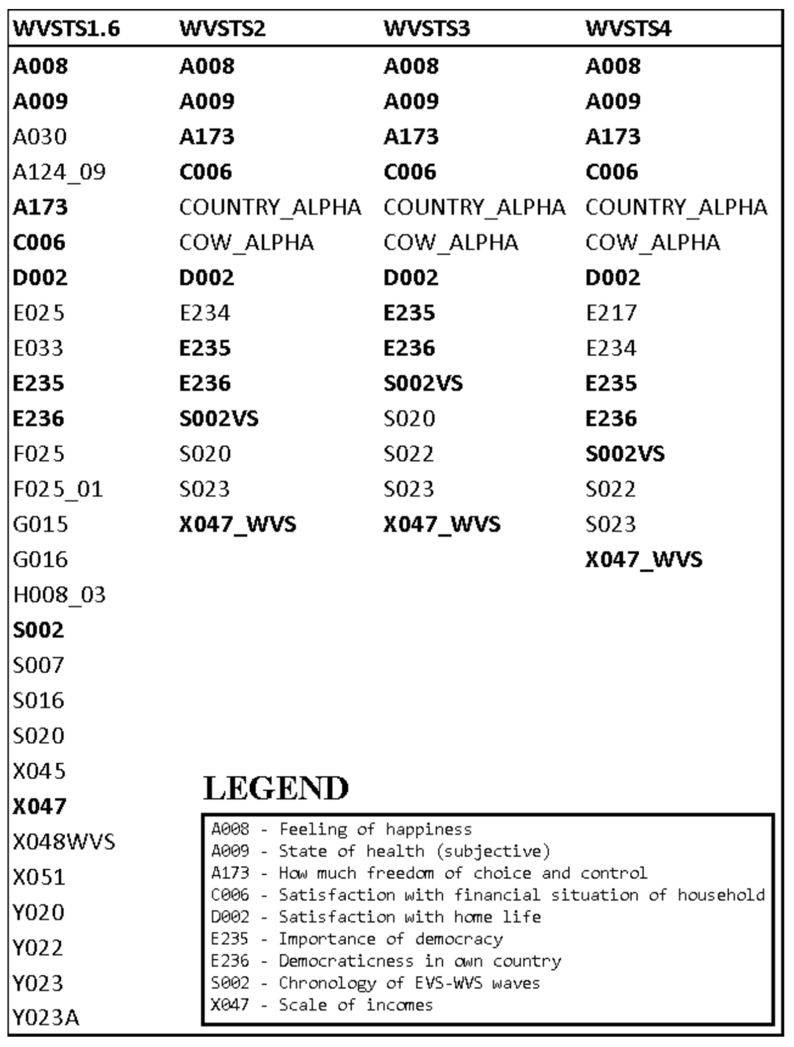
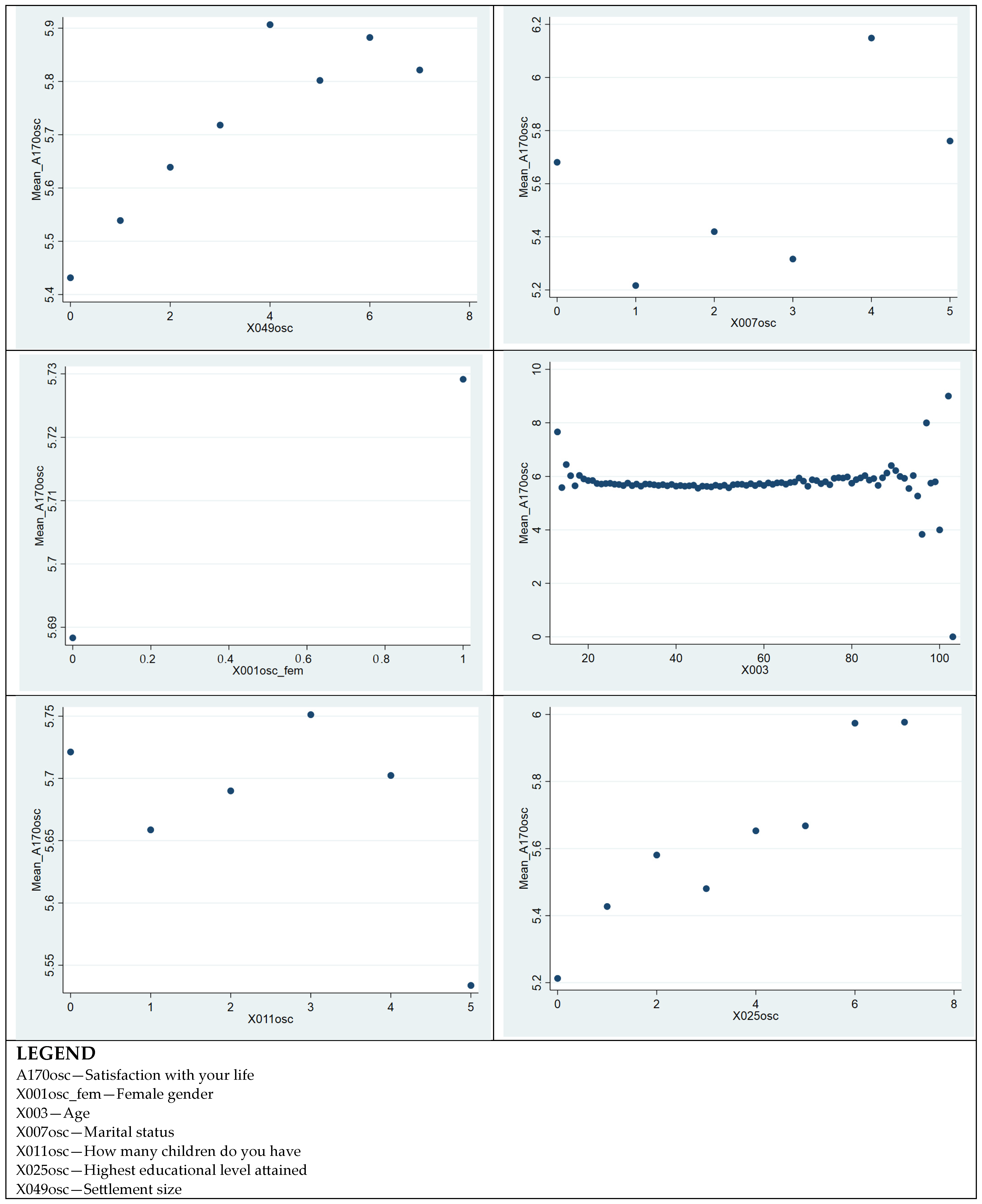
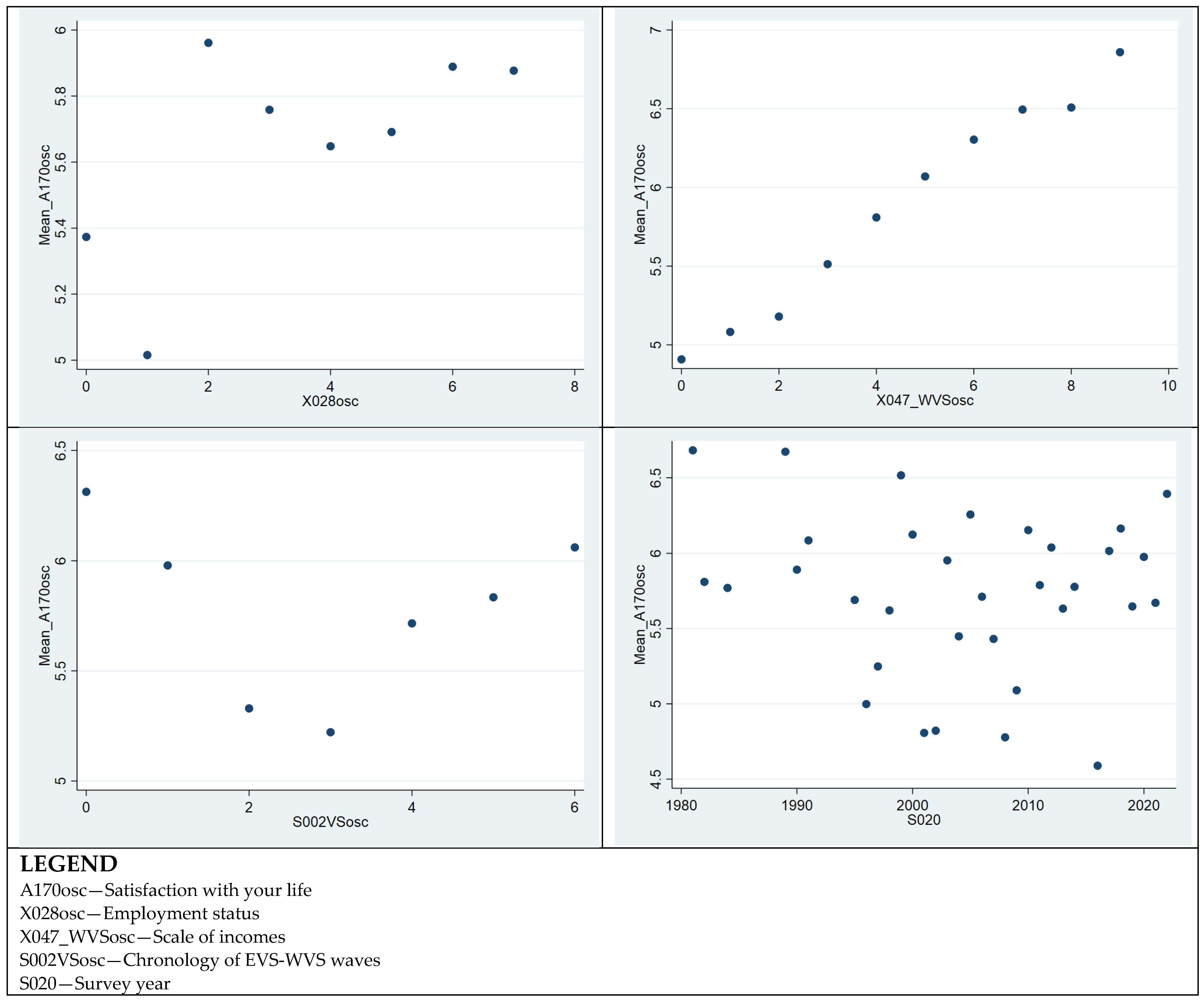
Disclaimer/Publisher’s Note: The statements, opinions and data contained in all publications are solely those of the individual author(s) and contributor(s) and not of MDPI and/or the editor(s). MDPI and/or the editor(s) disclaim responsibility for any injury to people or property resulting from any ideas, methods, instructions or products referred to in the content.

© 2024 by the author. Licensee MDPI, Basel, Switzerland. This article is an open access article distributed under the terms and conditions of the Creative Commons Attribution (CC BY) license (https://creativecommons.org/licenses/by/4.0/).

Share and Cite

MDPI and ACS Style

Homocianu, D. Life Satisfaction: Insights from the World Values Survey. Societies 2024, 14, 119. https://doi.org/10.3390/soc14070119

AMA Style

Homocianu D. Life Satisfaction: Insights from the World Values Survey. Societies. 2024; 14(7):119. https://doi.org/10.3390/soc14070119

Chicago/Turabian Style

Homocianu, Daniel. 2024. "Life Satisfaction: Insights from the World Values Survey" Societies 14, no. 7: 119. https://doi.org/10.3390/soc14070119

Note that from the first issue of 2016, this journal uses article numbers instead of page numbers. See further details here.

Article Menu

Life Satisfaction: Insights from the World Values Survey

Abstract

1. Introduction

2. Related Work

3. Materials and Methods

4. Results

5. Discussion

5.1. Main Findings

5.2. Socio-Demographic Findings

6. Limitations and Future Research Directions

7. Conclusions

Funding

Institutional Review Board Statement

Informed Consent Statement

Data Availability Statement

Conflicts of Interest

List of Abbreviations

Appendix A

Notes

References

Share and Cite

Article Metrics

Article Access Statistics

Further Information

Guidelines

MDPI Initiatives

Follow MDPI