Nonlinear Analysis of Steel Structure Bent Frame Column Bearing Transverse Concentrated Force at the Top in Factory Buildings

Abstract

The steel bent frame structure of single-story factory buildings is actually a spatial structure system. Different bent frame columns are connected with the roof of bent frame structure, making the columns work and bearing the load together. In the steel frame of the factory building with bridge cranes below 20 t, variable-section columns with corbels are used to bear the crane load. In this article, the steel bent frame column of single-story factory buildings was taken as the research object. The bent frame column was simplified as a cantilever variable stepped column bearing a transverse concentrated force at the top. After simplifying the model, the theoretical formula of deflection, rotating angle, and bending moment of the compression rod was put forward. Moreover, bending deformation and stability of variable stepped columns were analyzed in order to obtain the theoretical and practical formula, then the ANSYS software was used to simulate the bent column.

1. Introduction

Due to the high standardization and short construction period, the steel bent frame structure of single-story factory buildings is widely used in our daily life. Until the last 10 years of the last century, steel structure was only adopted by factory buildings with heavy-duty in China. To satisfy the needs of large tonnage cranes, the main bearing system of steel structure is composed of variable stepped columns and roof trusses. With the increase of steel production, more and more factory buildings with light-duty also adopted steel structures, which are mainly variable-section columns with corbels [1,2].

In terms of the force on the steel bent frame column, Ma [2] elaborated the plane bent frame through the design of single-story factory buildings and determined the calculation procedures of the schematic load, the internal force analysis of the column section, and the internal force combination, but the theoretical formula of model simplification was not given. M. Rezaiee-pajand [3] discussed the performance of supporting the frame system under gravity and lateral loads, and explained and calculated the displacement of the frame under transverse load by applying the virtual work method. Their study focused on the analysis of the tapered beam column with a functionally graded section. Using two different methods, both second-order effects and flexibility of connections were considered in the analysis. However, the effect of torsion and bending deformation was not investigated. In Ding [4] introduced the MS-TMM for the analysis of the elastic-plastic responses of the bending structure of a new single-story frame during rarely occurring earthquakes. The elastic-plastic response spectrum was directly used in seismic design to calculate the elastic-plastic response of the structure under a rare earthquake. The general expression of elastic-plastic response spectrum was deduced by the theoretical analysis and the application method of elastic-plastic response spectrum in the earthquake action calculation was proposed, but the exact shape function of the frame was not put forward. Under the self-weight of the roof or other live loads and the concentrated wind loads, the steel bent frame column can be simplified as a model with a compression rod, namely, a cantilever variable stepped column bearing transverse concentrated force at the top. As for compression bars, Euler and Lagrange first analyzed the nonlinear buckling of straight rods under end loads. Later, relevant studies also were conducted by many researchers [5,6,7]. Among them, the parametric solution for the elasticity of straight rods under compression and coupling was successfully proposed by Griner [5]. Based on the theory of elastic mechanics, the parametric solution for the nonlinear buckling analysis problem of a continuous rod with an elastic support was given. The nonlinear and buckling analysis of an elastic continuous bar on elastic supports, subjected to terminal compressive forces, was presented by assuming that the compressive forces and the flexural rigidities may vary from one span to the next. The strongly nonlinear equilibrium differential equation of each deformed member was formulated and through convenient boundary and compatibility conditions, the equations with unknowns was formulated, which was further enriched by a set of three-moment equations [6]. A fast algorithm for Euler’s elastica functional was proposed [7], in which the Euler’s elastica functional was reformulated as a constrained minimization problem. Combining the augmented Lagrange method and operator splitting techniques, the resulting saddle-point problem was solved by a serial of sub-problems. Nevertheless, the variable cross-section members and the plastic deformation were not taken into consideration in their work.

In view of the above shortcomings, the change of section shape and the influence of bending deformation on the stability of compression bar were taken into consideration. A series of theoretical formulas for model simplification and the shape function of the bent column of factory buildings were obtained through the bending deformation of the second-order cantilever variable order column. In this article, the bending deformation and stability analysis of the second-order cantilever variable stepped column bearing transverse concentrated force at the top were conducted. The theoretical formulas of the deflection, rotating angle, and bending moment were derived using the analytic method for compression rod bending. By applying the continuous and boundary conditions, the solution of the bending equilibrium differential equation, which is the shape function, was obtained. The stability of the variable stepped column was also analyzed. The ANSYS finite element software was used to analyze the engineering case and simulate the stress of a single bent column. Under the joint action of transverse and longitudinal loads, the location of the maximum shear force, displacement and maximum stress of the bent column with two cross-sections, namely H-section and the rectangular section bent column were obtained, which were used to verify the applicability of the theoretical formula, so as to provide practical application significance for the derivation of the formula. It is expected to provide a theoretical basis for the nonlinear stability calculation of the steel bent column of second-order factory buildings under the joint action of transverse and longitudinal loads.

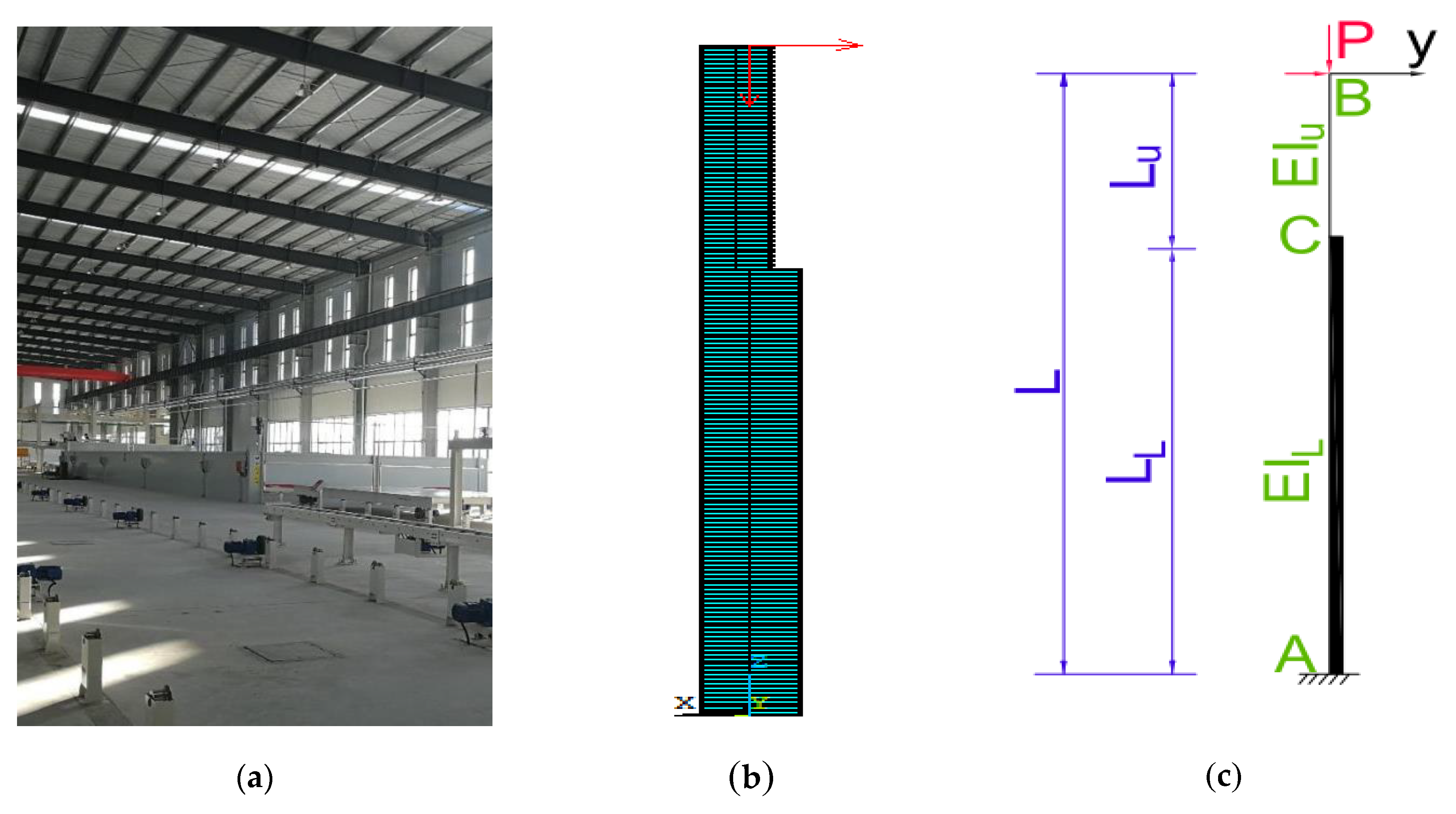
2. Model Simplification

Through the ANSYS modeling software (Ansys 18.2, Mechanical APDL Product Launcher 18.2, USA), the force of the steel bent frame column is simulated in this paper. First, the unit type is selected as a beam element. In order to obtain a simple model before loading, the material properties are defined, points and lines are created, and the mesh is divided. Restriction and axial pressure $P$ are applied on it, and the top of the column is also subjected to a horizontal force $Q_0$, which simulates the force of the steel bent frame column under the actual conditions. The detailed drawing 1(b) is as follows in Figure 1. After the calculation is completed, the stress cloud diagram of the model is obtained through post-processing. The stress cloud diagram is discussed below. The structural components of the device in actual engineering are relatively complex, and the mechanical effects in some details are not ideal.

In order to make the mechanical model simple and scientific, the model needs to be simplified. Simplify the model in the ANSYS software to a cantilever variable-step column with a lateral concentrated force at the top. Diagram 1(c) is shown in Figure 1. Next, analyze the model diagram and derive a series of formulas.

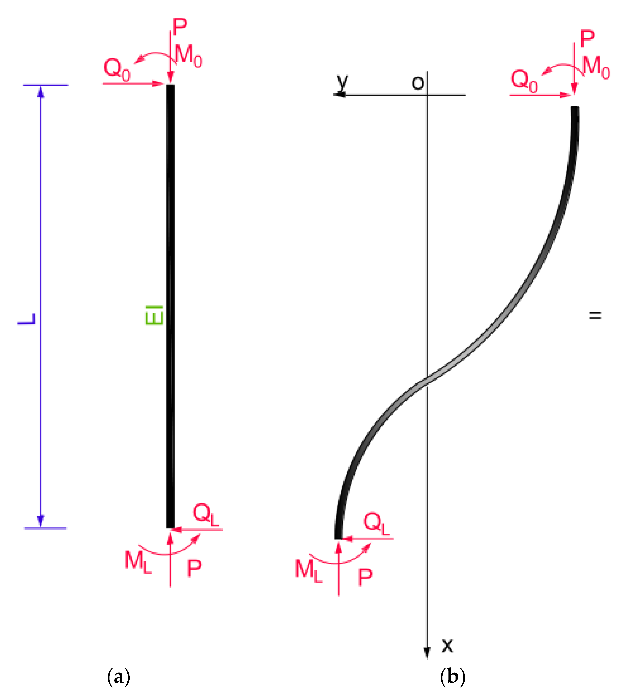
3. Basic Equation of the Model

3.1. Solution of the Differential Equation of the Deflection Curve

First, the basic formula for the compression rod bending should be derived. A straight compression rod with equal sections was taken out from the elastic structure, and any constraints were imposed at both ends, so that there were the axial force, shear force, and bending moment on the end section, as shown in Figure 2. In the figure, the original vertical position without the load was presented by the straight line, while the new balanced position under the load was shown by the curve [8,9].

An endpoint before deformation was taken out as the original point of X-axis, another end as the positive direction of X-axis. The direction in which the original end was shifted was regarded as the positive direction of Y-axis. Therefore, a rectangular plane coordinate system is established, which was called the unit coordinate system of the compression rod.

In the analysis of stability, the axial pressure of the rod was usually calculated only in a numerical value, without the negative sign, such as Euler’s critical load $P_E={\pi }^{2}EI/L^2$. In this article, the example was followed and the axial pressure was picked as positive. When the direction of shear force $Q_0$ at the $O$ end of the rod was consistent with the direction of Y-axis, it was picked as positive, otherwise it was negative. When the direction of shear force $Q_L$ at the L end of the rod was consistent with the direction of Y-axis, it was picked as negative, otherwise it was positive. As ruled in this study, the bending moment was positive if the curvature was negative, that is, the bending moment that made the Y-axis positive side edge on the cross section generate tensile stress was stipulated as the positive bending moment, otherwise it was negative.

In the unit coordinate system, the differential equation for the bending equilibrium is:

$$EI\frac{d^{2}y}{d{x}^2}+P\left(y-y_0\right)=-M_0+Q_{0}x$$

(1)

where $P$ is the axial force, $M_0$ and $Q_0$ are respectively the counter-torque and horizontal counter-force under the constraint on the section $x=0$, and y₀ is the horizontal displacement on the section $x=0$.

$E$ is the elastic modulus, and $I$ is called the sectional moment of inertia.

The general solution of the above differential Equation [10] is:

$$y=A_1\cos kx+A_2\sin kx+A_{3}x+A_4$$

(2)

where $k=\sqrt{P/EI}$, $A_i$ (i = 1, 2, 3, 4) is the undetermined integration constant, which can be determined by the boundary condition.

Introduce a parameter as follows:

$$\frac{A_1}{A_2}=-\tan \phi =-\frac{\sin \phi }{\cos \phi }$$

(3)

Sort out the above formula and introduce another coefficient $A$:

$$\frac{A_1}{-\sin \phi }=\frac{A_2}{\cos \phi }=A$$

(4)

It can be derived separately that:

$$A_1=-A\sin \phi ,A_2=A\cos \phi$$

Substitute the above formula into Equation (2) as follows:

$$y=A\sin \left(kx-\phi \right)+A_{3}x+A_4$$

(5)

The above expression is composed of two parts, namely a sine curve $A\sin \left(kx-\phi \right)$ and a sloping straight line $A_{3}x+A_4.$ Since the bending of the compression rod is a nonlinear problem, and the simple superposition method cannot be applied to the nonlinear problem [11,12], the necessary and sufficient condition on which the above two deflection expressions can be superposed is that they are all under the working condition subjected to the vertical load $P$ [13], as shown in Figure 3. Figure 3b–d suggests that the deflection curve in Figure 3b of the compression rod can be decomposed into two parts, that is the sine curve shown in Figure 3c—the deformation deflection curve of the rod under vertical load $P$ and bending moment $M$ at the rod end [14], and the sloping straight line in Figure 3d—the deflection expression of the deflection rod in the linear equilibrium state under vertical load $P$ and horizontal shear force $Q_0$ and $Q_L$ at the end of the rod.

Introduce a new parament $\mu$ which can be called the effective length coefficient of the rod, and $\mu L$μL is the distance between two points of inflection of the sine curve in Figure 3c. As shown in Figure 3c, the section between the two inflection points is a typical Euler bending model with a two-force rod [15,16], as follows:

$$P=\frac{{\pi }^{2}EI}{{\left(\mu L\right)}^2}$$

(6)

Substitute the above formula into the expression of $k$:

$$k=\sqrt{\frac{\frac{{\pi }^{2}EI}{{\left(\mu L\right)}^2}}{EI}}=\frac{\pi }{\mu L}$$

(7)

In Figure 3b, the expression of the bending moment at any section of the compression rod is:

$$M=PA\sin \left(kx-\phi \right)$$

(8)

Introduce a new parameter $\zeta$ which can be called the position coefficient of the inflection point. $\zeta L$ represents the distance from the first inflection point in the positive direction of the X-axis to the coordinate origin. As shown in Figure 3b, at the inflection point, substitute $x=\zeta L,M=0$ into the expression of the bending moment in Equation (8), as follows:

$$k\zeta L-\phi =0$$

Substitute the expression of $k$ into the above formula, as follows:

$$\phi =\frac{\zeta }{\mu }\pi$$

(9)

Substitute Equations (7) and (9) into Equation (5), the bending deflection curve equation of the compression rod represented by geometric parameters can be obtained:

$$y=A\sin \left(\frac{x}{\mu L}-\frac{\zeta }{\mu }\right)\pi +A_{3}x+A_4$$

(10)

The above formula is the general solution for the deflection curve differential Equation (1), which is suitable for the compression rods under any boundary conditions. For compression rods under boundary conditions, the process of striving for a particular solution can be transformed into the process of determining the geometric parameters of the deflection curve equation according to the continuous deformation condition of the rod end and the equilibrium condition for force.

3.2. Mechanical Significance of Basic Elements

Now, the basic property of the two basic elements—sine curve and sloping straight line which constitutes the deflection curve equation of the compression rod are analyzed. Considering $x=\zeta L$ and $x=\left(\mu +\zeta \right)L$, sine curve $A\sin \left(\frac{x}{\mu L}-\frac{\zeta }{\mu }\right)\pi =0,$ and the inflection points of the sine curve are all on the X-axis, so $A\sin \left(\frac{x}{\mu L}-\frac{\zeta }{\mu }\right)\pi$ is a sine curve with X-axis as the baseline. The distance between two inflection points on the sine curve is $\mu L$ and $\zeta L$ is the coordinate of the inflection point nearest to the positive direction of the origin. Since the maximum value of $A\sin \left(\frac{x}{\mu L}-\frac{\zeta }{\mu }\right)\pi$ is 1, A is the maximum deflection of the sine curve. In this state, the essence of force and deformation is a two-force rod in the curve balance (Euler bending balance). The most important geometric parameter of the sine curve effective length coefficient can be gained by Equation (6) as follows:

$$\mu =\sqrt{\frac{\frac{{\pi }^{2}EI}{L^2}}{P}}$$

(11)

The sloping straight line $A_{3}x+A_4$ is the only posture to keep the balance under the action of $P$ and $Q_0$ or $Q_L$ at both ends of the rod. $A_3$ in geometric meaning represents the tangent of the angle between the sloping straight line and X-axis, that is, the tangent of the angle between the resultant force line of $P$ and $Q_0$ at the end $O$ of the rod and X-axis, and its value is:

$$A_3=\frac{Q_0}{P}$$

(12)

As shown in Figure 3d, the force and deformation of the rod are essentially two-force rods under the state of linear balance. The intercept on Y-axis of the sloping straight line is represented by $A_4$ in the geometric meaning.

Usually, $A_3\ne 0,\zeta \ne 0,$ the origin of the rectangular coordinate system can be set at an endpoint of the rod before deformation. The X-axis of the rectangular coordinate system coincides with the rod axis. Another end of the rod is the positive direction of X-axis, and the direction of Y-axis is consistent with the deflection direction of the end $O$. In the rectangular coordinate system, if there is $A_3\ne 0,\zeta \ne 0,$ then $A_4=A_3\zeta L.$ If $A_3$ or $\zeta$ is zero, then $A_4$ must be determined by the boundary conditions.

In special cases, the origin of the rectangular coordinate system can be set at the rod end where the bending moment is zero. In this rectangular coordinate system, $A_4=0,\zeta =0$, and the calculation could be simplified.

From Equation (10), the tangent of the angle between the tangent direction at any point on the deflection curve and the X-axis can be obtained:

$$\tan \theta =\frac{dy}{dx}=A\frac{\pi }{\mu L}\cos \left(\frac{x}{\mu L}-\frac{\zeta }{\mu }\right)\pi +A_3$$

(13)

The bending moment at any point on the deflection curve of the rod is:

$$M=-EI\frac{d^{2}y}{d{x}^2}=PA\sin \left(\frac{x}{\mu L}-\frac{\zeta }{\mu }\right)\pi$$

(14)

4. Formula Reduction

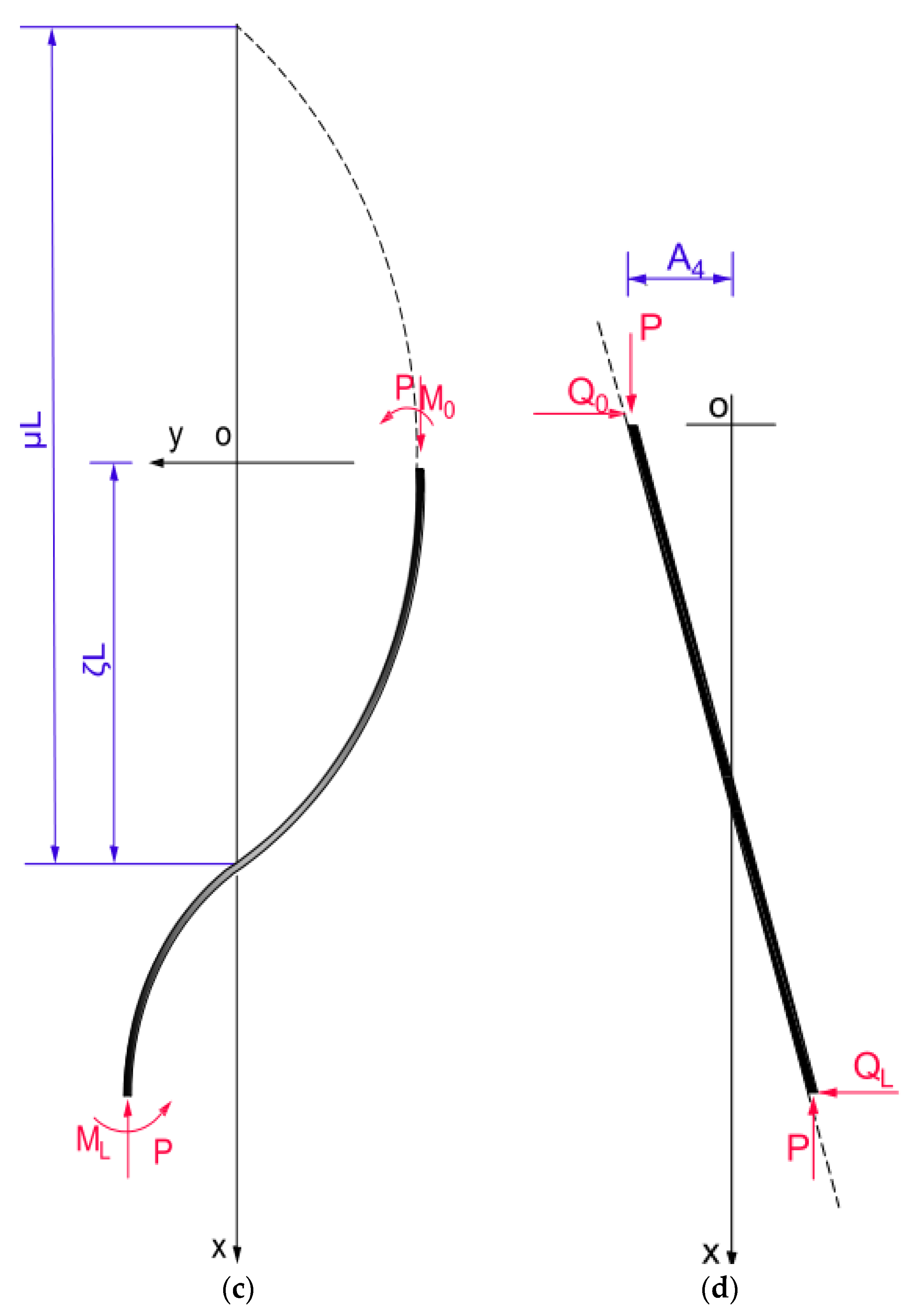
4.1. Analysis of Bending Deformation

As shown in Figure 4, the steel structure bent frame column of single-story factory buildings is simplified as a cantilever variable stepped column bearing transverse load at the top [17]. Figure 4a is the force diagram. The upper column is free while the bottom is fixed. $L$ is the height and $E$ is the elastic modulus. The length of the upper column is $L_u$ and the cross section moment of inertia is $I_u$. The length of the lower column is $L_l$ and the cross section moment of inertia is $I_l$. The centroid of the top section of the column is subjected to axial pressure $P$ and a horizontal force $Q_0$ acts at the top of the column [18,19,20]. Figure 4b is the diagram of deflection curve of the rod after deformation. The sine curve and sloping straight line after the decomposition of the bending deformation deflection curve are shown in Figure 4c,d.

The top of the column is seen as the origin and the axis of the column before deformation as X-axis. A rectangular plane coordinate system is established in this way that the direction of the fixed end is regarded as the positive direction of X-axis. In addition, the lateral deflection direction of the rod is the positive direction of Y-axis.

As shown in Figure 4c, the upper and lower parts of the column are segmented for analysis. The axial force $P$ acts on both upper and lower parts, so the calculating length coefficient of the sine curve after decomposition can be calculated by $P$, namely:

$${\mu }_u=\sqrt{\frac{{\pi }^{2}E{I}_u}{P{L}^2}},{\mu }_l=\sqrt{\frac{{\pi }^{2}E{I}_l}{P{L}^2}}$$

(15)

Divide the above two formulas, then:

$$\frac{{\mu }_u}{{\mu }_l}=\sqrt{\frac{I_u}{I_l}}$$

(16)

As shown in Figure 4c, extend the sine curve of the upper and lower column, respectively, it can be seen that the difference between $I_u$ and $I_l$ of the two curves results in the different distances between two inflection points. The deformation is continuous and the two sine curves are tangent at the connecting variable section of the upper and lower column.

Since the shear force at the $O$-end of the rod is $Q_0$, the tangent value of the angle between the sloping straight line after decomposition and X-axis is $A_3=Q_0/P$. Substitute $A_3=Q_0/P$ into the basic equation of deflection curve (10) of the compression rod, so the deflection curve of the upper column can be written as follows:

$$y_u=A_u\sin \left(\frac{x}{{\mu }_{u}L}-\frac{{\zeta }_u}{{\mu }_u}\right)\pi +\frac{Q_0}{P}x+A_{4u}$$

(17)

The rotating angle equation and bending moment equation of the upper column can be respectively expressed as follows:

$$\tan {\theta }_u=A_u\frac{\pi }{{\mu }_{u}L}\cos \left(\frac{x}{{\mu }_{u}L}-\frac{{\zeta }_u}{{\mu }_u}\right)\pi +\frac{Q_0}{P}$$

(18)

$$M_u=P{A}_u\sin \left(\frac{x}{{\mu }_{u}L}-\frac{{\zeta }_u}{{\mu }_u}\right)\pi$$

(19)

Given the boundary condition, the bending moment of end $O$ is zero. Substitute $x=0,M_{u0}=0$ into the above formula, ${\zeta }_u=0$ can be obtained [21]. Therefore, the deflection curve equation, rotating equation, and bending moment equation of the upper column can be written as follows:

$$y_u=A_u\sin \frac{x}{{\mu }_{u}L}\pi +\frac{Q_0}{P}x+A_{4u}\left(0\le x\le L_u\right)$$

(20)

$$\tan {\theta }_u=A_u\frac{\pi }{{\mu }_{u}L}\cos \frac{x}{{\mu }_{u}L}\pi +\frac{Q_0}{P}\left(0\le x\le L_u\right)$$

(21)

$$M_u=P{A}_u\sin \frac{x}{{\mu }_{u}L}\pi \left(0\le x\le L_u\right)$$

(22)

Substitute $x=L_u$ into the above three formulas, the deflection, rotating angle, and bending moment at the variable section are as follows:

$$y_c=A_u\sin \frac{L_u}{{\mu }_{u}L}\pi +\frac{Q_0}{P}{L}_u+A_{4u}$$

(23)

$$\tan {\theta }_c=A_u\frac{\pi }{{\mu }_{u}L}\cos \frac{L_u}{{\mu }_{u}L}\pi +\frac{Q_0}{P}$$

(24)

$$M_u=P{A}_u\sin \frac{L_u}{{\mu }_{u}L}\pi$$

(25)

The axial force and shear force acting on the lower column are the same as that on the upper column, so the angle between the sloping straight line decomposed from the deflection curve and the X-axis is the same as that of the upper bar. According to the basic equation of deflection curve of the compression rod in Equation (10), the deflection curve equation of the lower column can be obtained as follows:

$$y_l=A_l\sin \left(\frac{x}{{\mu }_{l}L}-\frac{{\zeta }_l}{{\mu }_l}\right)\pi +\frac{Q_0}{P}x+A_{4l}\left(L_u\le x\le L\right)$$

(26)

The rotating angle equation and the bending moment equation of the lower column can be written as follows:

$$\tan {\theta }_l=A_l\frac{\pi }{{\mu }_{l}L}\cos \left(\frac{x}{{\mu }_{l}L}-\frac{{\zeta }_l}{{\mu }_l}\right)\pi +\frac{Q_0}{P}\left(L_u\le x\le L\right)$$

(27)

$$M_l=P{A}_l\sin \left(\frac{x}{{\mu }_{l}L}-\frac{{\zeta }_l}{{\mu }_l}\right)\pi \left(L_u\le x\le L\right)$$

(28)

Substitute $x=L_u$ into the above three formulas, the deflection, rotating angle, and bending moment at the variable section are obtained respectively as follows:

$$y_c=A_l\sin \left(\frac{L_u}{{\mu }_{l}L}-\frac{{\zeta }_l}{{\mu }_l}\right)\pi +\frac{Q_0}{P}{L}_u+A_{4l}$$

(29)

$$\tan {\theta }_c=A_l\frac{\pi }{{\mu }_{l}L}\cos \left(\frac{L_u}{{\mu }_{l}L}-\frac{{\zeta }_l}{{\mu }_l}\right)\pi +\frac{Q_0}{P}$$

(30)

$$M_c=P{A}_l\sin \left(\frac{L_u}{{\mu }_{l}L}-\frac{{\zeta }_l}{{\mu }_l}\right)\pi$$

(31)

The turning angle of the upper and lower column is continuous at section $C$, combining Equation (24) with Equation (30) then sorting it out as follows:

$$\frac{A_u}{{\mu }_u}\cos \frac{L_u}{{\mu }_{u}L}\pi =\frac{A_l}{{\mu }_l}\cos \left(\frac{L_u}{{\mu }_{l}L}-\frac{{\zeta }_l}{{\mu }_l}\right)\pi$$

(32)

The bending moment of the upper and lower column is equal at section $C$, combining Equation (25) with Equation (31) then sorting it out as follows:

$$A_u\sin \frac{L_u}{{\mu }_{u}L}\pi =A_l\sin \left(\frac{L_u}{{\mu }_{l}L}-\frac{{\zeta }_l}{{\mu }_l}\right)\pi$$

(33)

Divide and sort out the above two formulas as follows:

$$\tan \frac{L_u}{{\mu }_{u}L}\pi =\frac{{\mu }_l}{{\mu }_u}\tan \left(\frac{L_u}{{\mu }_{l}L}-\frac{{\zeta }_l}{{\mu }_l}\right)\pi$$

(34)

In the above formula, only ${\zeta }_l$ is an unknown number. Therefore, the position coefficient of the lower column reflex point can be derived as follows:

$${\zeta }_l=\frac{L_u}{L}-\frac{{\mu }_l}{\pi }\arctan \left(\frac{{\mu }_u}{{\mu }_l}\tan \frac{L_u}{{\mu }_{u}L}\pi \right)$$

(35)

The rotation angle at the fixed end is zero. Substitute $x=l,{\theta }_{lL}=0$ into the rotation angle equation of the lower bar, then:

$$\tan {\theta }_{lL}=A_l\frac{\pi }{{\mu }_{l}L}\cos \left(\frac{1}{{\mu }_l}-\frac{{\zeta }_l}{{\mu }_l}\right)\pi +\frac{Q_0}{P}=0$$

(36)

It can be obtained from the above formula that:

$$A_l=-\frac{\frac{Q_0}{P}·\frac{{\mu }_l}{\pi }·L}{\cos \frac{{\zeta }_l-1}{{\mu }_l}\pi }$$

(37)

Substitute the above formula into Equation (33) as follows:

$$A_u=-\frac{\frac{Q_0}{P}·\frac{{\mu }_l}{\pi }·L·\sin \left(\frac{L_u}{{\mu }_{l}L}-\frac{{\zeta }_l}{{\mu }_l}\right)\pi }{\cos \frac{{\zeta }_l-1}{{\mu }_l}\pi ·\sin \frac{L_u}{{\mu }_{u}L}\pi }$$

(38)

The deflection of the fixed end is zero. Substitute $x=L$ into the deflection curve equation of the lower column, then:

$$y_{lL}=A_l\sin \left(\frac{1}{{\mu }_l}-\frac{{\zeta }_l}{{\mu }_l}\right)\pi +\frac{Q_0}{P}L+A_{4l}=0$$

(39)

Substitute Equation (37) into the above formula and sort out, so $A_{4l}$ can be expressed as follows:

$$A_{4l}=\frac{Q_{0}L}{P}\left(-\frac{{\mu }_l}{\pi }\tan \frac{{\zeta }_l-1}{{\mu }_l}\pi -1\right)$$

The deflection of the upper and lower column at the variable section is equal, combining Equation (23) with Equation (29), then:

$$A_u\sin \frac{L_u}{{\mu }_{u}L}\pi +\frac{Q_0}{P}{L}_u+A_{4u}=A_l\sin \left(\frac{L_u}{{\mu }_{l}L}-\frac{{\zeta }_l}{{\mu }_l}\right)\pi +\frac{Q_0}{P}{L}_u+A_{4l}$$

(40)

Substitute Equation (33) into the above formula:

$$A_{4u}=A_{4l}$$

(41)

The above formula suggests that the intercept on the Y-axis of the sloping straight line decomposed from the deflection curve of the upper and lower column is equal. It has been discussed before that the slope of the sloping straight line decomposed from the deflection curve of the upper column is the same as that of the lower one. Therefore, the two sloping straight lines coincide with each other perfectly. It can also be concluded from Figure 4b,c that the deflection curve of the upper and lower column at section $C$ is continuous, so the sine curve and the sloping straight line after decomposition at this variable section is continuous.

After the geometric parameters and integral constants are determined, the deflection curve equation, rotation angle equation, and bending moment equation of the upper column can be written as follows:

$$y_u=\frac{Q_{0}L}{P}\left[-\frac{{\mu }_l}{\pi }\tan \frac{{\zeta }_l-1}{{\mu }_l}\pi -1+\frac{x}{L}+\frac{{\mu }_l\sin \frac{{\zeta }_{l}L-L_u}{{\mu }_{l}L}\pi ·\sin \frac{x}{{\mu }_{u}L}\pi }{\pi \cos \frac{{\zeta }_l-1}{{\mu }_l}\pi ·\sin \frac{L_u}{{\mu }_{u}L}\pi }\right]\left(0\le x\le L_u\right)$$

(42)

$$\tan {\theta }_u=\frac{Q_0}{P}\left[1+\frac{{\mu }_l\sin \frac{{\zeta }_{l}L-L_u}{{\mu }_{l}L}\pi ·\cos \frac{x}{{\mu }_{u}L}\pi }{{\mu }_u\cos \frac{{\zeta }_l-1}{{\mu }_l}\pi ·\sin \frac{L_u}{{\mu }_{u}L}\pi }\right]\left(0\le x\le L_u\right)$$

(43)

$$M_u=\frac{Q_{0}L{\mu }_l\sin \frac{{\zeta }_{l}L-L_u}{{\mu }_{l}L}\pi ·\sin \frac{x}{{\mu }_{u}L}\pi }{\pi \cos \frac{{\zeta }_l-1}{{\mu }_l}\pi ·\sin \frac{L_u}{{\mu }_{u}L}\pi }\left(0\le x\le L_u\right)$$

(44)

The deflection curve equation, rotation angle equation, and bending moment equation of the lower column can be expressed as follows:

$$y_l=\frac{Q_{0}L}{P}\left[-\frac{{\mu }_l}{\pi }\tan \frac{{\zeta }_l-1}{{\mu }_l}\pi -1+\frac{x}{L}+\frac{{\mu }_l\sin \frac{{\zeta }_{l}L-x}{{\mu }_{l}L}\pi }{\pi \cos \frac{{\zeta }_l-1}{{\mu }_l}\pi }\right]\left(L_u\le x\le L\right)$$

(45)

$$\tan {\theta }_l=\frac{Q_0}{P}\left[1-\frac{\cos \frac{{\zeta }_{l}L-x}{{\mu }_{l}L}\pi }{\cos \frac{{\zeta }_l-1}{{\mu }_l}\pi }\right]\left(L_u\le x\le L\right)$$

(46)

$$M_l=\frac{Q_{0}L{\mu }_l\sin \frac{{\zeta }_{l}L-x}{{\mu }_{l}L}\pi }{\pi \cos \frac{{\zeta }_l-1}{{\mu }_l}\pi }\left(L_u\le x\le L\right)$$

(47)

Substitute $x=0$ into (42), the deflection at the top of the column is:

$$y_{max}=y_0=\frac{Q_{0}L}{P}\left(-\frac{{\mu }_l}{\pi }\tan \frac{{\zeta }_l-1}{{\mu }_l}\pi -1\right)$$

(48)

In Equation (47), the bending moment expression of the upper column at any section can be determined by the axial force $P$ and shear force $Q_0$ at the top of the column as follows:

$$M_u=-P\left(y_0-y_u\right)-Q_{0}x$$

(49)

Substitute Equations (48) and (42) into the above formula, the results obtained are the same as in (44). In the same way, the bending moment expression of the lower column at any section can be determined by the axial force $P$ and shear force $Q_0$ at the top of the column as follows:

$$M_l=-P\left(y_0-y_l\right)-Q_{0}x$$

(50)

Substitute Equations (48) and (45) into the above formula, and the same result as in (47) is obtained. After further verification, the deflection curve, rotation angle, and bending moment equation of the upper and lower column inferred from the analytic method satisfy the continuous condition at the variable section, the boundary condition of the zero rotation angle and displacement at the fixed end, and the condition of zero bending moment at the top of the column.

4.2. Stability Analysis

Consider $P$ as a variable and analyze the stability of the variable stepped column [22]. From the displacement expression (48) at the top of the column, the column will get unstable when the value of $\tan \frac{{\zeta }_l-1}{{\mu }_l}\pi$ approaches infinity [23]. The precondition that $\tan \frac{{\zeta }_l-1}{{\mu }_l}\pi$ approaches infinity is that $\cos \frac{{\zeta }_l-1}{{\mu }_l}\pi$ approaches zero, meaning that the deflection will increase rapidly when ${\zeta }_l=\frac{{\mu }_l}{2}+1$. Substitute ${\zeta }_l=\frac{{\mu }_l}{2}+1$ into Equation (34) and sort it out, then:

$$\tan \frac{L_u}{{\mu }_{u}L}\pi ·\tan \left[\frac{L_l}{{\mu }_{l}L}·\sqrt{\frac{I_u}{I_l}}\right]\pi =\sqrt{\frac{I_l}{I_u}}$$

(51)

4.3. Promotion

In this paper, the theoretical formulas of lateral displacement, rotation angle, and bending moment of second order cantilever variable order column can also be extended and applied for the N-order variable order columns.

5. ANSYS Modeling Analysis

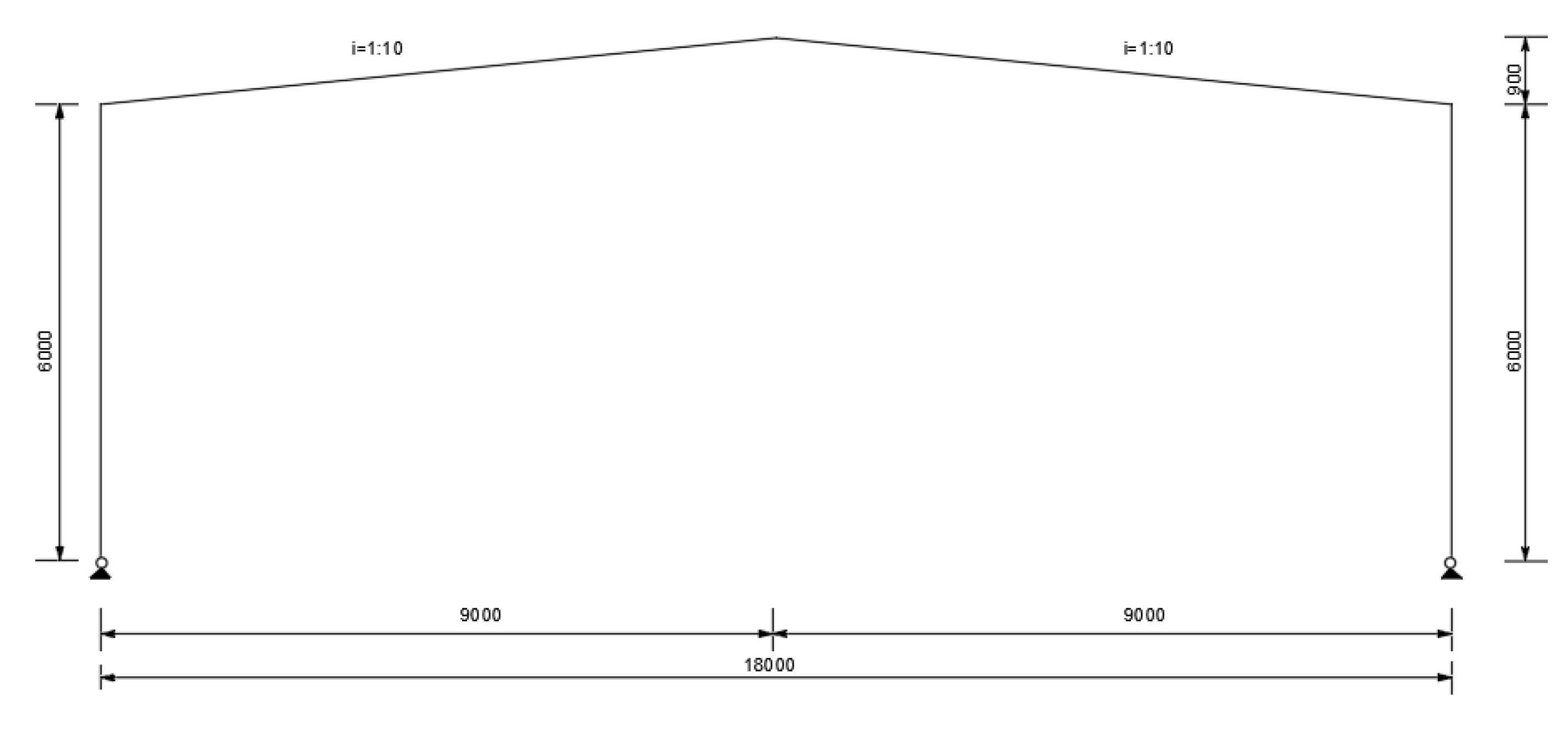
5.1. Model Simplification

The structural components of the device in actual engineering are relatively complex, and the mechanical effects in some details are not ideal. In order to make the mechanical model simple and scientific, the model needs to be simplified. In this paper, the structural member is a variable-step column with the top end bearing the lateral concentrated force, so the model is built by the beam element.

5.2. Parameter Selection

The unit type of H-section of the bent column is Beam 188, Q235, the elastic modulus is 200 GMPa, and Poisson’s ratio is 0.3.

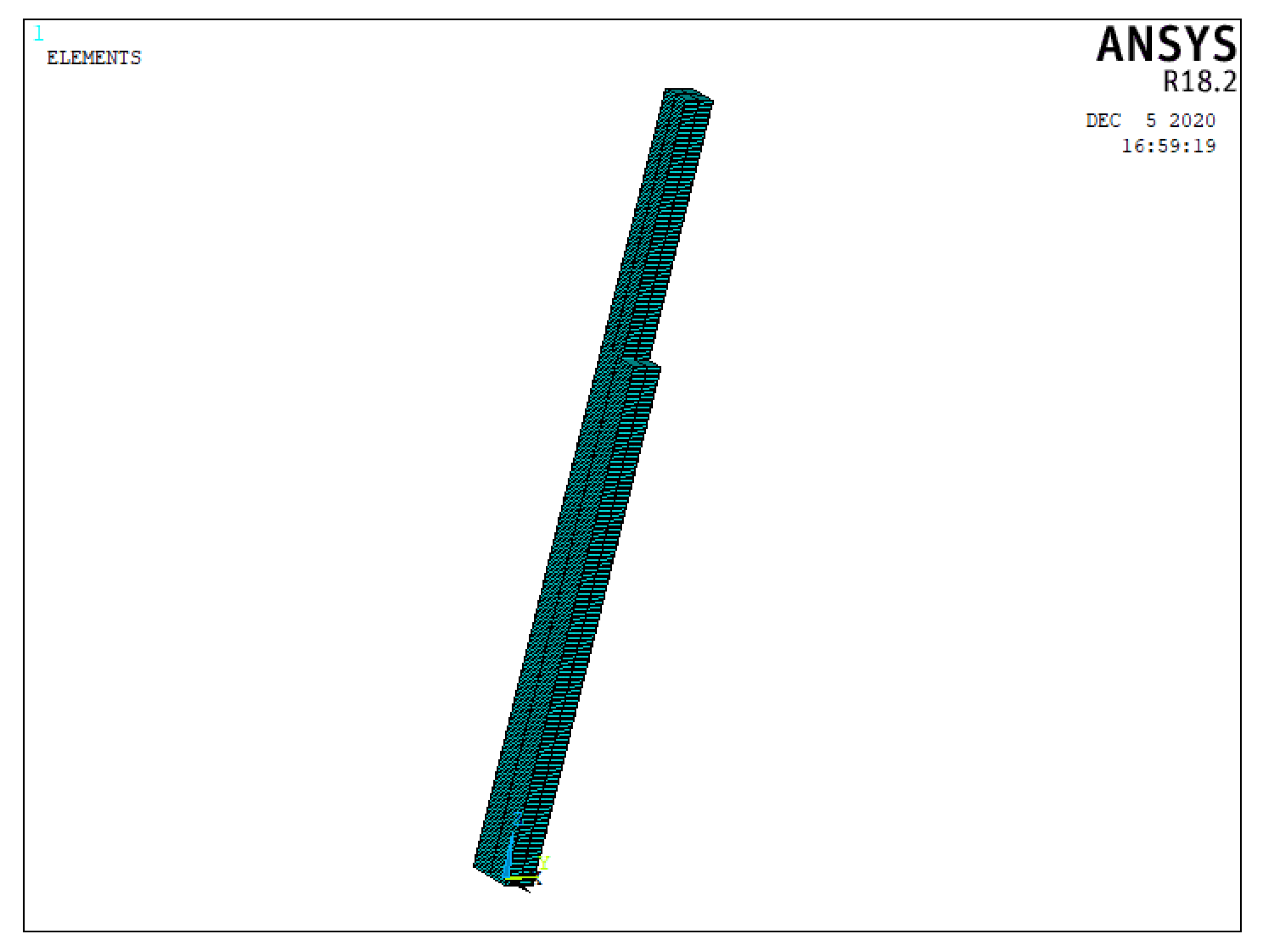
5.3. ANSYS Solid Structure Modeling

The solid structure of the single-story light steel workshop is a single span and double slope portal frame with a transverse span of 18 m and a column height of 6 m. There are eight frames in the house, with a column spacing of 6 m and a roof slope of 1/10. The safety level of the house is grade II with Q235. The overall form of the rigid frame is shown in Figure 5.

The frame column is made of H-shaped steel, in which the length of the lower column is 4 m, and the size is 500 mm × 400 mm × 6 mm × 10 mm. While the length of the upper column is 2 m, and the size is 350 mm × 250 mm × 6 mm × 10 mm. A single bent column model is selected for numerical simulation. In this model, three key points are selected to determine one line. Then, grid division is carried out where the unit length is defined as 20 mm, and the upper and lower columns are divided into 100 and 200 units, respectively. The denser grids help indicate the changes of displacement and stress. The divided grid is shown in Figure 6.

The other is a rectangular section of the reinforced concrete column. The elastic modulus is 30,000 MPa and Poisson’s ratio is 0.2. The height of the lower column is 4 m, b × h = 250 mm × 400 mm, and upper column height is 2 m, b × h = 250 mm × 250 mm. The mesh size is 20 mm. The upper and lower columns are divided into 100 and 200 parts, respectively. The grid after division is shown in Figure 7.

For the load calculation, the longitudinal load and transverse loads mainly include.

(1)

Roof dead load: 0.3 KN/m² (including the dead weight of the profiled steel sheet and purlin).

(2)

Roof live load: 0.5 KN/m².

(3)

Horizontal load of crane: Bridge crane with a lifting capacity of 10 t and working system of A3.

(4)

Wind load: The basic wind pressure is 0.4 KN/m² and the ground roughness is class A.

(5)

Snow load: The basic snow pressure is 0.2 KN/m², which is less than the uniform live load on the roof, so it is not considered.

According to the theoretical calculation and empirical analysis, it is assumed that the longitudinal load on the plant is about 20 t, which is, 200,000 N, and the transverse load is about 2000 N. The bottom of the bent column is restrained in three directions, and the load on the top of the column is the superposition of transverse and longitudinal loads.

5.4. Comment

The structural models with different cross-sections affect the nonlinear finite element analysis. Actually, any numerical model will be affected by model uncertainty. For some beams, such as Beam SL, Beam SH, and Beam CLX (S = Square, L = Low enhancement ratio, M = Medium enhancement ratio, H = High enhancement ratio) the failure mode does not present any modifications. The design ultimate loads provided by GRF (Resistance factor) and PFM (Partial factor method) safety formats are always lower than those evaluated by the PM (Probability method). Moreover, for the Beam CLX, the ECOV (Coefficient of variation) safety format also provides a design ultimate load lower than that estimated by PM. Instead, for the other beams (i.e., Beam SM and T-Beam) the failure modes are characterized by some modifications. In fact, for the Beam SM, only the GRF safety format provides a lower design ultimate load than that recommended by PM. The estimated value by PFM is very close to that by PM, but it is slightly unsafe. For the T-Beam, all the estimated design ultimate loads by GRM (General resistance method) safety formats (i.e., PFM, ECOV, GRF, and GSF) are higher than that estimated by PM, which is believed to be less reliable, since GRM is not able to capture the modifications in the failure mode [24].

6. Result Analysis

6.1. H-Section

6.1.1. Shear Force

Under the combined action of transverse and longitudinal loads, the shear diagram of the bent column is locally enlarged, as shown in Figure 8. Due to the large cross-sectional area of the lower column, the structure remains relatively stable, and the shear force distribution in this part is relatively uniform. On the contrary, due to the smaller cross-sectional area, there is a concentrated load directly acting on the upper column. The shear force in the lateral direction is seriously uneven. The shear force of the side where the concentrated force is present is large, while the other side is much smaller. Moreover, the maximum shear force is 8.19304 N at the side of the joint where the concentrated force is present, and the minimum shear force is 49.1136 N at the other side. This is caused by the weak steel bent structure at the variable section.

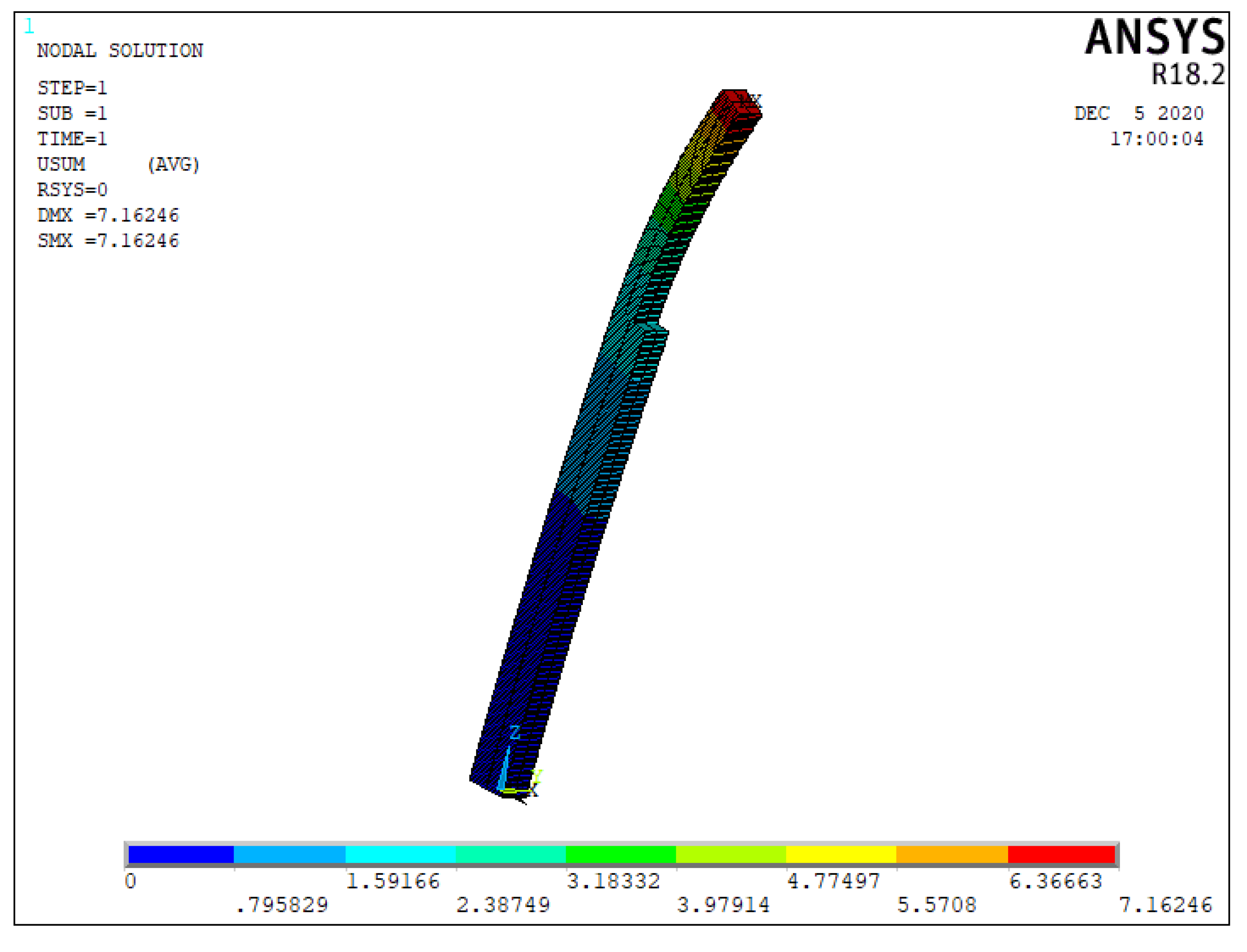
6.1.2. Displacement

After the ANSYS simulation calculation is performed on the variable-order column model with the transverse load and longitudinal load, the stress cloud diagram is obtained. The total displacement diagram is shown in Figure 9. The maximum displacement occurs at the top of the column and its value is 2.5944 mm. It can be seen that the results of the numerical simulation are consistent with the shape function of bent columns derived from the theoretical formula. The displacement increases gradually along the column from the bottom to the top. The maximum displacement occurs at the top of the column, and the maximum displacement ranges from 2.31 to 2.59 mm. Therefore, it can be concluded that the deformation of the top of the bent structure column of the workshop is slight, which meets the requirements of structural reliability.

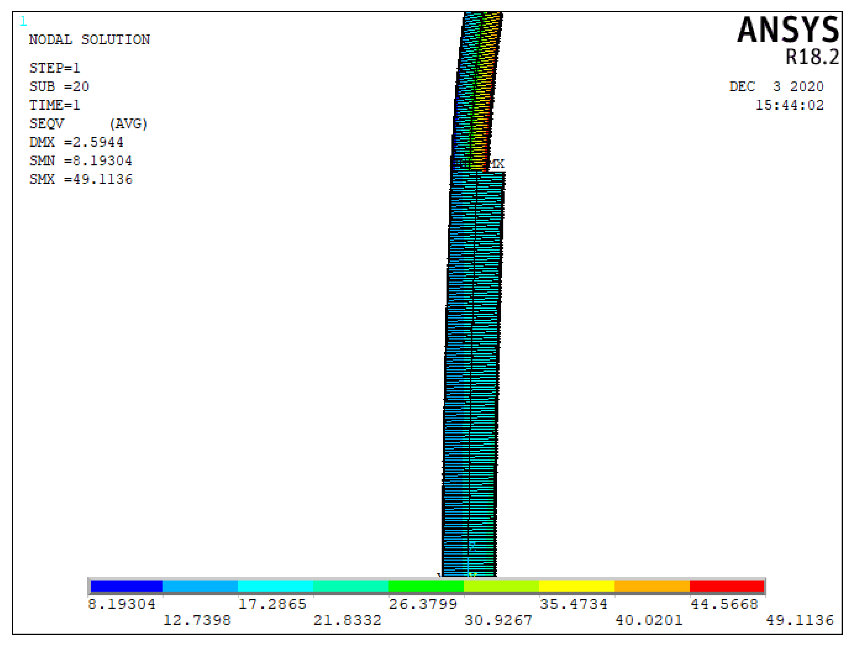
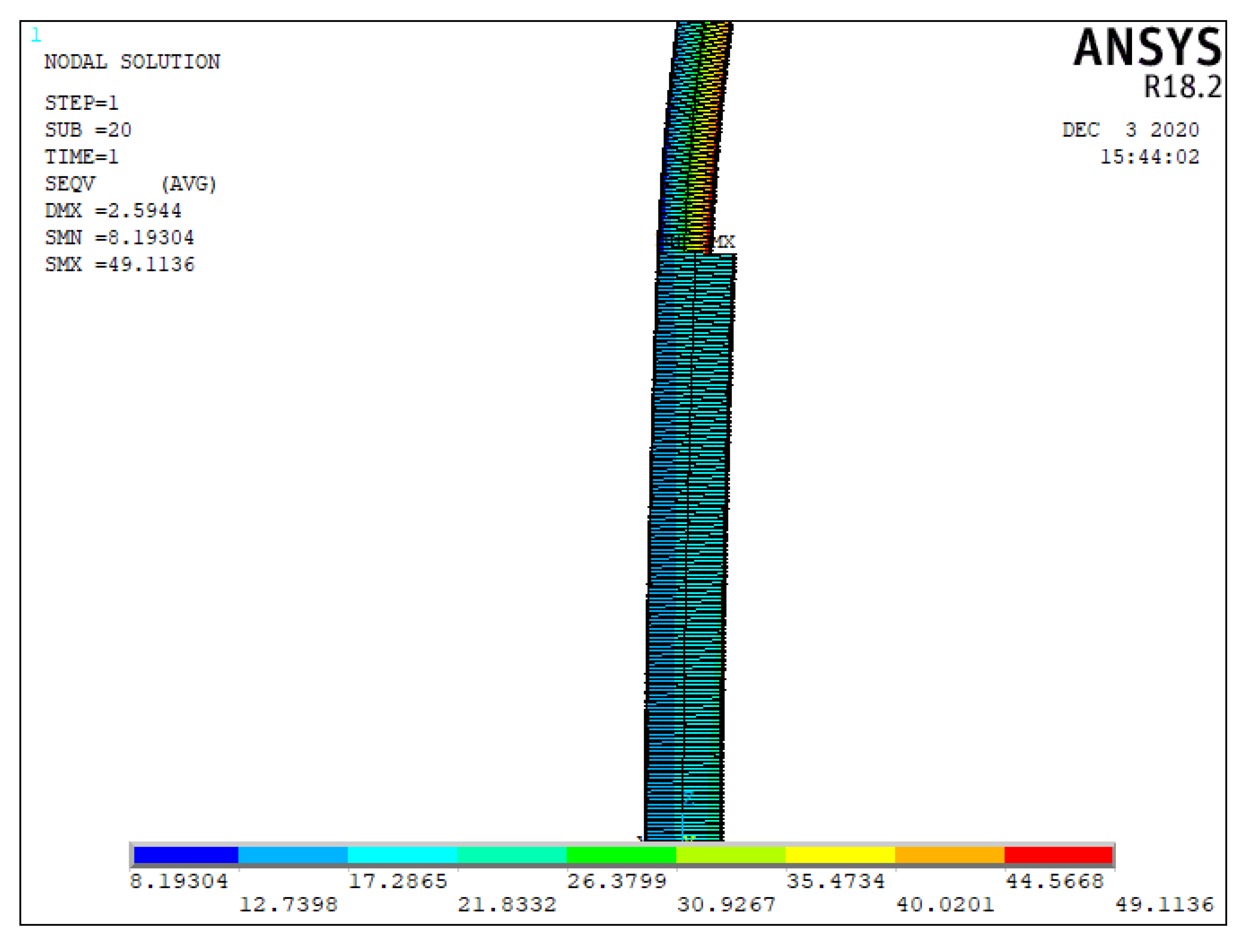
6.1.3. Stress

After the ANSYS simulation calculation performed on the variable-order column model with the transverse load and longitudinal load, the stress cloud diagram is obtained. The Mises stress diagram is shown in Figure 10. The maximum stress is 49.1136 MPa and the minimum stress is 8.19304 MPa. Owing to a large cross-sectional area of the lower column, the structure is relatively stable and the stress distribution is uniform. The cross-sectional area of the upper column is small and there is a concentrated load directly acting on it. The stress on the side with the concentrated force is small, but the other side produces a larger stress. Moreover, the maximum stress is 49.1136 MPa at the side of the joint with the concentrated force, and the minimum stress is 8.1930 MPa at the other side. This is due to the steel bent structure at the variable cross-section, which is relatively weak.

6.1.4. Summary

Through the above numerical simulation, it can be seen that the maximum displacement (2.5944 mm) of the steel bent column with H-section occurs at the top of the column, and the deformation meets reliability requirements. The maximum shear force occurs at the variable section side where the concentrated force is produced, which is 8.19304 N, while the maximum stress occurs at the other side, which is 49.1136 MPa. This is due to the discontinuity of the steel bent column at the variable section and the weak structure.

6.2. Rectangular Section

Displacement

The stress nephogram of the variable order column model with transverse and longitudinal loads is obtained after the ANSYS simulation calculation. The total displacement figure is shown in Figure 11. The maximum displacement occurs at the top of the column, and its value is 7.16246 mm. It can be seen that the numerical simulation results are consistent with the shape function of bent columns derived from the theoretical formula. The displacement increases gradually along the column height from the column base up. The maximum displacement ranges from 6.37 to 7.16 mm. In general, the deformation at the top of the bent structure column is larger than that of the H-section, which may be due to the smaller section size. However, its deformation is still a small deformation, which meets the requirements of structural reliability.

7. Conclusions

The plane steel structure bent frame calculation plays an important role in the design of single-story factory buildings. The steel bent frame column with corbels is a bending component under variable axial forces. The top of the column is subjected to the weight of the roof structure, the roof live load, the snow load, and the longitudinal force (including longitudinal seismic forces, concentrated wind load) [25], which is characterized by the difference between the sections of the upper and lower part. The length and load of the upper part are much smaller than that of the lower one.

In this paper, the differential equation for bending balance in Equation (1) was established through the model simplification of the steel structure bent frame column in factory buildings. In addition, the general solution of differential equation of the compression rod in Equation (10) which could be applied to any boundary condition was derived. It can be seen from the analytical expressions that the deflection curve was decomposed into a sine curve and a sloping straight line, suggesting that the compression rod issue is a nonlinear one. Moreover, the steel bent frame column was simplified as a cantilever variable stepped column bearing transverse concentrated force at the top. The correct solution of the differential equation was obtained by employing the continuous condition at the variable sections of the upper and lower columns and the boundary condition of the fixed end. The instability analysis of variable order columns is carried out. Finally, the model is established by the ANSYS finite element method to simulate the stress of the single bent column. Under the joint action of the transverse and longitudinal loads, the position of maximum shear force, displacement, and maximum stress of the bent column with two cross-sections, namely H-section and the rectangular section bent column are obtained, which gives the derivation of the theoretical formula practical application significance, and also provides a theoretical basis for the design and calculation of the steel bent column of the second-order, single-story factory buildings under the joint action of the transverse and longitudinal loads.

References

- Chen, S.F. Effective length of columns with corbel in mill building frames. J. Build. Struct. 2007, 28, 54–60. [Google Scholar]
- Ma, X.Q. Calculation of plane shelving in the design of single-layer workshop. J. Lanzhou Petrochem. Coll. Technol. 2015, 15, 39–42. [Google Scholar]
- Rezaiee-Pajand, R. Stability Analysis of Frame Having FG Tapered Beam-Column. Int. J. Steel Struct. 2019, 19, 446–468. [Google Scholar] [CrossRef]
- Ding, J.G.; Dai, Y.W.; Qiao, Z. Analysis of elastic-plastic responses of a new single-story frame-bent structure during an earthquake based on the transfer matrix method of multibody system. Adv. Mech. Eng. 2013, 5, 452–462. [Google Scholar] [CrossRef] [Green Version]
- Griner, G.M. A parametric solution of the elastic pole-vaulting pole problem. J. Appl. Mech. ASME 1984, 51, 409–414. [Google Scholar] [CrossRef]
- Panayotounakos, D.E. Nonlinear and buckling analysis of continuous bars lying on elastic supports, based on the theory of elastiea. Ing. Arch. 1986, 56, 351–361. [Google Scholar] [CrossRef]
- Duan, Y.; Wang, Y.; Tai, X.C.; Hahn, J. A Fast Augmented Lagrangian Method for Euler’s Elastica Model. In Scale Space and Variational Methods in Computer Vision; Springer: Berlin/Heidelberg, Germany, 2012; pp. 144–156. [Google Scholar]
- Audoly, B.; Callan-Jones, A.; Brun, P.T. Dynamic curling of an Elastica: A nonlinear problem in elastodynamics solved by matched asymptotic expansions. In Extremely Deformable Structures; Springer: Vienna, Austria, 2015; pp. 137–155. [Google Scholar]
- Liu, Y.; Yan, T.; Li, C. Stress and Deflection Analysis of a Complicated Frame Structure with Special-Shaped Columns. In Information Computing and Applications; Springer: Berlin/Heidelberg, Germany, 2010; pp. 282–288. [Google Scholar]
- Jin, M.; Bao, Z.B. An improved proof of instability of some Euler elasticas. J. Elast. 2015, 121, 303–308. [Google Scholar] [CrossRef]
- Yang, Y.B. Research on nonlinear, postbuckling and elasto-plastic analyses of framed structures and curved beams. Meccanica 2020, 1–26. [Google Scholar] [CrossRef]
- Bigoni, D.; Bosi, F.; Misseroni, D.; Dal Corso, F.; Noselli, G. New phenomena in nonlinear elastic structures: From tensile buckling to configurational forces. In Extremely Deformable Structures; Springer: Vienna, Austria, 2015; pp. 55–135. [Google Scholar]
- Mostafa, R.S. Predictive modeling of the lateral drift capacity of circular reinforced concrete columns using an evolutionary algorithm. Eng. Comput. 2019, 1–13. [Google Scholar] [CrossRef]
- Xu, G.S.; Wu, B.; Jia, D.D.; Xu, X.T.; Yang, G. Quasi-static tests of RC columns under variable axial forces and rotations. Eng. Struct. 2018, 162, 60–71. [Google Scholar] [CrossRef]
- Miura, T. Elastic curves and phase transitions. Math. Ann. 2020, 376, 1629–1674. [Google Scholar] [CrossRef] [Green Version]
- Morozov, N.F.; Tovstik, P.E. Dynamic Buckling of a Rod under Longitudinal Load Lower Than the Eulerian Load. Dokl. Ross. Akad. Nauk 2014, 453, 282–285. [Google Scholar]
- Plaut, R.H.; Virgin, L.N. Optimal design of cantilevered elastica for minimum tip deflection under self-weight. Struct. Multidiscip. Optim. 2011, 43, 657–664. [Google Scholar] [CrossRef]
- Farzad, H. Moment Resistance System. In Analysis Procedure for Earthquake Resistant Structures; Springer: Singapore, 2018; pp. 1–226. [Google Scholar]
- Farzad, H. Braced Steel Frame System. In Analysis Procedure for Earthquake Resistant Structures; Springer: Singapore, 2018; pp. 227–340. [Google Scholar]
- Farzad, H. Frames with Shear Wall. In Analysis Procedure for Earthquake Resistant Structures; Springer: Singapore, 2018; pp. 341–448. [Google Scholar]
- Vetyukov, Y.; Schmidrathner, C. A rod model for large bending and torsion of an elastic strip with a geometrical imperfection. Acta Mech. 2019, 230, 4061–4075. [Google Scholar] [CrossRef] [Green Version]
- Gao, K.; Gao, W.; Wu, D. Nonlinear dynamic stability analysis of Euler–Bernoulli beam–columns with damping effects under thermal environment. Nonlinear Dyn. 2017, 90, 2423–2444. [Google Scholar] [CrossRef]
- Belyaev, A.K.; Morozov, N.F.; Tovstik, P.E. Buckling problem for a rod longitudinally compressed by a force smaller than the Euler critical force. Mech. Solids 2016, 51, 263–272. [Google Scholar] [CrossRef]
- Castaldo, P.; Gino, D.; Mancini, G. Safety formats for nonlinear finite element analysis of reinforced concrete structures: Discussion, comparison and proposals. Eng. Struct. 2019, 193, 136–153. [Google Scholar] [CrossRef]
- Yin, L. Elementary discussion on calculation of support between columns of single-story and multi-span concrete bent factory buildings. City Build. 2014, 4, 58–71. [Google Scholar]
Publisher’s Note: MDPI stays neutral with regard to jurisdictional claims in published maps and institutional affiliations. |
© 2020 by the authors. Licensee MDPI, Basel, Switzerland. This article is an open access article distributed under the terms and conditions of the Creative Commons Attribution (CC BY) license (http://creativecommons.org/licenses/by/4.0/).
Share and Cite
Li, C.; Wang, L.; Weng, Y.; Qin, P.; Li, G. Nonlinear Analysis of Steel Structure Bent Frame Column Bearing Transverse Concentrated Force at the Top in Factory Buildings. Metals 2020, 10, 1664. https://doi.org/10.3390/met10121664
Li C, Wang L, Weng Y, Qin P, Li G. Nonlinear Analysis of Steel Structure Bent Frame Column Bearing Transverse Concentrated Force at the Top in Factory Buildings. Metals. 2020; 10(12):1664. https://doi.org/10.3390/met10121664
Chicago/Turabian StyleLi, Chunbao, Lina Wang, Yongmei Weng, Pengju Qin, and Gaojie Li. 2020. "Nonlinear Analysis of Steel Structure Bent Frame Column Bearing Transverse Concentrated Force at the Top in Factory Buildings" Metals 10, no. 12: 1664. https://doi.org/10.3390/met10121664
APA StyleLi, C., Wang, L., Weng, Y., Qin, P., & Li, G. (2020). Nonlinear Analysis of Steel Structure Bent Frame Column Bearing Transverse Concentrated Force at the Top in Factory Buildings. Metals, 10(12), 1664. https://doi.org/10.3390/met10121664