Article

Benchmarks for Accelerated Cyclic Plasticity Models with Finite Elements

by
Jelena Srnec Novak
1,*,
Francesco De Bona
1 and
Denis Benasciutti
2
1
Polytechnic Department of Engineering and Architecture (DPIA), University of Udine, via delle Scienze 206, 33100 Udine, Italy
2
Department of Engineering, University of Ferrara, via Saragat 1, 44122 Ferrara, Italy
*
Author to whom correspondence should be addressed.
Metals 2020, 10(6), 781; https://doi.org/10.3390/met10060781
Submission received: 12 May 2020 / Revised: 28 May 2020 / Accepted: 8 June 2020 / Published: 11 June 2020

Abstract

:
In numerical simulations of components subjected to low-cycle fatigue loading, the material cyclic plasticity behavior must be modelled until complete stabilization, which occurs approximately at half the number of cycles to failure. If the plastic strain per cycle is small, a huge number of cycles must be simulated, which results into a huge and thus unaffordable simulation time. Acceleration techniques for shortening this time are useful, although their accuracy needs to be checked. This work aims to compare different approaches (nonlinear kinematic with “initial” and “stabilized” parameters and combined nonlinear kinematic and isotropic with the speed of stabilization fictitiously increased). It considers two benchmarks taken from the literature, in which the material has opposite cyclic behaviors (hardening, softening). A plane finite element model can be used in both benchmarks, thus permitting a simulation up to complete stabilization. Results confirm that the common approach of considering only the kinematic model (calibrated on “initial” or “stabilized” material state) from the very first cycle could lead to relevant errors. The acceleration technique based on a fictitious increase in the speed of stabilization leads to accurate results. Guidelines for calibrating this technique on a material’s hardening or softening behavior are, finally, proposed.

1. Introduction

Structural components can be subjected to mechanical and/or thermal cyclic loading conditions, which often lead to stress redistribution in structures with localized plasticity regions. Correct prediction of the local stress–strain history is quite important to estimate the low-cycle fatigue life of components as accurately as possible. The finite element (FE) method has been proved to be a convenient tool for this purpose.
A crucial aspect in FE modelling of components undergoing low-cycle fatigue is the choice of an appropriate elasto-plastic material model. Over the last few decades, several cyclic plasticity models have been proposed [1,2,3,4,5,6], and most of them are already implemented in commercial FE software. The constitutive material model should be able to represent as closely as possible the material behavior observed during experimental testing. It is also worth noting that it is possible to estimate the durability of a structure subjected to cyclic loading only if it has reached its steady state response (i.e., complete material stabilization) [7]. Some metallic materials stabilize approximately at half the number of cycles to failure [7], whereas other materials never stabilize completely [8]. In either case, if the plastic strain is small, materials would exhibit a rather slow evolution of their properties and, therefore, a huge number of cycles must be simulated. When the complexity of the component geometry also leads to an FE model with a relevant number of degrees of freedom, the simulation of the cycle-by-cycle model response could require unfeasible computational time. Such evidence has been recently reported in [9], for notched 316 steel samples. Several block loading histories were applied to achieve stabilization. Local ratcheting curves up to stabilization were simulated with FE analysis. Results obtained with the Ahmadzadeh-Varvani (A-V) kinematic hardening model were compared with measured values.
Some alternative methods have thus been proposed in the literature to alleviate the above-mentioned computational burden. Some authors [10,11] have suggested that only a few cycles be simulated. This procedure, although not well defined, seems suitable if a thermal loading with creep is imposed, as the presence of visco-elasticity generally tends to significantly reduce the time to stabilization. A different approach has been proposed by [12,13], who suggest using a kinematic model with stabilized material properties already from the beginning of FE analysis. Some other authors have proposed more sophisticated approaches with an attempt to follow the material evolution from the initial transient up to stabilization. An extrapolation technique, which significantly reduces the calculation time, has been developed by [14], if creep constitutes the damage criterion. To evaluate the stabilized cyclic behavior directly, the direct cyclic algorithm (DCA) was developed in [15]. DCA uses a combination of Fourier series and time integration of the nonlinear material behavior to obtain the stabilized response of a component iteratively [16]. As pointed out in [16], due to the characteristics of DCA and the inevitable numerical error caused by the approximation and convergence problem, this method seems not always able to provide accurate solutions for complicated engineering problems. As an alternative acceleration procedure, the cycle-jumping procedure has been devised in [17,18]. This technique makes use of the Taylor’s expansion to bypass the calculation of some intermediate cycles, based on the fact that the stress redistribution is quite small over time. Even if quite promising, this approach has not yet been implemented in commercial code and thus requires a heavy additional programming effort. Finally, in [19], the material property evolution is accelerated by fictitiously increasing a parameter that governs the speed of stabilization in the presence of creep, and for either cyclic hardening or softening behavior. Despite its simplicity, this method seems able to preserve the physics of the cycle-by-cycle evolution of material properties. Furthermore, the method appears to be useful, especially in cases dealing with materials that exhibit a rather slow cyclic evolution like in [20].
In the present study, this latter accelerated technique was investigated by considering different material behaviors and loading conditions. For this purpose, two different case studies are presented: a mold for continuous casting of steel (cyclic softening, thermal loading) and a cruciform welded joint (cyclic hardening, displacement-controlled loading). These two cases were selected from those available in the literature, as they are characterized by a quite simple geometry that also allows a complete simulation without an accelerated technique to be performed, to be used as a reference.

2. Theoretical Background of Cyclic Plasticity Models

The elasto-plastic material behavior under cyclic loading can be represented by a combined kinematic and isotropic material model. A kinematic model captures the Bauschinger effect, since it assumes that, under a progressive yielding, the yield surface translates in the stress space (see Figure 1a), at the same time maintaining a constant size [1,2,3,4,5,6]. By contrast, the isotropic model (see Figure 1b) assumes that, at any stage of loading, the center of the yield surface remains at the origin and it expands homothetically in size as plastic strain develops.
The von Mises yield surface can be represented as [1,2,3,4,5,6]:
3 2 ( S X ) : ( S X ) R σ 0 = 0
where S is the deviatoric stress tensor, X is the backstress (kinematic) tensor, R is the drag stress, and σ0 is the initial yield stress before any plastic deformation. The kinematic part (translation of the yield surface) is controlled by X, whereas the isotropic part (homothetic expansion of the yield surface) is managed by R.
Different kinematic models have been developed to relate the backstress X to the plastic strain εpl [1,2,3,4,5,6]. The Armstrong and Frederick (A-F) nonlinear kinematic model is described by the following equation [1,2,3,4,5,6]:
d X = 2 3 C d ε pl γ X d p
where C is the hardening modulus and γ is the recover parameter, which controls the decay of C in dependence on the accumulated plastic strain, p = (2/3 dεpl: dεpl)1/2. Decomposition of the backstress into several A-F models gives the Chaboche model [1,2,3,4,5,6]. Nevertheless, the A-F model already gives a satisfactory description of the material behavior considered in the present work, as can be seen in [8,21].
Very often, a nonlinear isotropic model (known also as the Voce model [22]) is adopted for modeling material strain hardening or softening. Expansion of the yield surface is described with the change in the drag stress R [1,2,3]:
R = R [ 1 exp ( b p ) ]
where b is the speed of stabilization and R is the stabilized stress. The stabilized stress can be positive or negative, representing either cyclic hardening (R > 0) or softening (R < 0), respectively. Evolution of R can also be interpreted as the relative change in the maximum stress σmax,i in the Nth cycle with respect to the maximum stress in the first (σmax,1) and in the stabilized (σmax,s) cycle [1,2,3,4]:
σ max , i σ max , 1 σ max , s σ max , 1 R R = 1 exp   ( b p )
The material stabilizes when R reaches R, which (according to [4]) occurs approximately when the exponent bp = 5. Obviously, as is also pointed out in [4], a more precise way to determine the material stabilization is to plot the normalized maxima (Equation (4)) as a function of the accumulated plastic strain for several low-cycle fatigue tests; see [23]. For the CuAg alloy presented in [23], the material stabilizes when the exponent is approximately in the range 4 ÷ 12. In case of strain-controlled loading, the plastic strain range per cycle ∆εpl is approximately constant and the plastic strain accumulated after N cycles becomes [1,4]:
p 2 Δ ε pl N
When the stabilized condition is reached, it is:
2 b N stab Δ ε pl 5
where Nstab is the number of cycles to stabilization. This relationship (6) shows that Nstab is inversely proportional to both b and Δεpl. Moreover, it shows that Nstab may become very large when b and Δεpl are both small.
Figure 2 plots Equation (4) versus the accumulated plastic strain (on a log scale) for different values of b. As can be noticed, by increasing the speed of stabilization b, the curve shifts to the left, while its “S-shape” remains essentially unaffected. In other words, a material with a higher value of b reaches its stabilized condition at a lower value of p (i.e., in a smaller number of cycles).
Following the recommendations of the literature (e.g., see [1,5]), the material parameters are calibrated on experimental data obtained with specimens under cyclic strain-controlled loading. However, a real component often exhibits a combination of both stress- and strain-controlled conditions that could have some effect on the final stabilized stress–strain response. In this case, calibration should possibly be tailored on the real stress–strain evolution.

3. First Case Study: Cyclic Softening Material Behavior and Thermal Loading

Steelmaking components are often subjected to thermo-mechanical loads applied cyclically. Typical examples are rolls for hot strip rolling, anodes in electric arc furnaces and molds for continuous casting [24,25,26].

3.1. Round Mold under Cyclic Thermal Flux

During the continuous casting process, the molten steel flows into a water-cooled mold. The mold controls the initial solidification of steel and the shape of semi-finished products. Different cross sections may be adopted (square, rectangular or rounded shapes) according to the geometry of the final product (billets, blooms or slabs). Due to the direct contact with the molten steel, the inner part of the mold is subjected to a high thermal flux with a characteristic profile decreasing from top to bottom; see Figure 3a. Consequently, large temperature gradients occur across the mold thickness, especially in the region near to the meniscus (free level of the liquid metal). Temperature gradients cause relevant elastic and plastic strains. The overall thermal flux distribution also changes over time, from its full value (when the plant is in service) to zero (when the plant is switched off); see Figure 3c. The component is simply supported, and it is free to expand. Molds are made of copper alloys, as they have a favorable combination of high thermal conductivity and good mechanical strength. This study considers a CuAg0.1 alloy (see Table 1), whose mechanical properties were experimentally obtained in [8].

3.1.1. Numerical Model of the Round Mold

The mold here investigated has a round cross-section (inner diameter: 200 mm, thickness: 16 mm) and is 1000 mm long, similar to the case presented by [27]. Due to axi-symmetry, a two-dimensional (2D) finite element model was adopted (see Figure 3a,b), thus strongly decreasing the computational time. The finite element model has 760 elements and 2487 nodes. The mesh was refined in the meniscus area (point “A”; see Figure 3b), where the highest temperatures and stress gradients are expected to occur. Firstly, a thermal analysis was performed to obtain the temperature distribution, which was used as an input in the subsequent mechanical analysis.
For the thermal analysis, plane elements with eight nodes were adopted. A thermal flux was imposed at the inner surface, while convection was considered on the outer surface to simulate the water cooling. The thermal flux q proposed in [27] was increased by around 50%, so that the mold reached a maximum temperature close to 300 °C. As a consequence, an increase in the amount of plastic strain was obtained. The temperature of the cooling water was 40 °C and the convection coefficient was 48,000 W/m2K. As observed in [25], the variation in the thermal flux can be approximated by simulating a sequence of steady-state analyses. A nonlinear solution was carried out to take into account the temperature dependence of thermal properties.
The maximum temperatures and thermal gradients occur in the region close to the meniscus in the location labeled with the letter “A” in Figure 3b.
The mechanical analysis was carried out after imposing, as thermal loading, the temperature distribution calculated in the thermal analysis. No mechanical constraints were applied to the model, as the actual mold is free to expand. Plane elements with eight nodes were used. The temperature dependence of material parameters was taken into consideration. A nonlinear combined kinematic (A-F) and isotropic (Voce) material model was used. Model parameters of the CuAg0.1 alloy are reported in Table 1.

3.1.2. Reference Case: Cyclic Behavior up to Stabilization

To establish a reference case, the nonlinear combined kinematic and isotropic model had to be brought up to complete stabilization. For this purpose, it is necessary to choose a criterion that establishes when material stabilization is reached. A possible solution is that of controlling the variation of stresses or strains from cycle to cycle. In general, the choice of the parameter to be monitored can be arbitrary. In this work, the two considered cases undergo low-cycle fatigue. Thus, after the numerical simulation, a durability analysis has to be performed by means of a Manson–Coffin curve and, consequently, the stabilization criterion was defined in terms of equivalent strain range [7]:
Δ ε eq = 2 3 [ Δ ( ε 1 ε 2 ) ] 2 + [ Δ ( ε 2 ε 3 ) ] 2 + [ Δ ( ε 3 ε 1 ) ] 2
where Δ(εiεj) is the range of the relative difference between principal strains εi and εj. The relative difference between the equivalent strain ranges in two subsequent cycles was calculated:
Δ r eq = ( | Δ ε eq ( i ) Δ ε eq ( i + 1 ) | Δ ε eq ( i ) ) × 100
and compared with a threshold value. According to the adopted criterion, the material stabilizes within 489 cycles, as can be also seen in Figure 4. For the critical point “A”, Figure 4a displays the axial, hoop and von Mises maximum stresses at each cycle, versus the number of cycles. In this location, “A”, the state of stress is biaxial, as the radial stress is obviously zero (free surface). In Figure 4b, the three components of strain range and the equivalent strain range are plotted as a function of the number of cycles. It can be observed that the hoop strain range is almost constant, whereas the other two components increase until stabilization. The equivalent strain range increases throughout the whole loading cycle, with a maximum rise of about 20%.
This behavior can be clearly detected in the evolution of hoop stress–strain cycles, as depicted in Figure 5. For more clarity, the figure only plots the first five cycles, the 50th, 75th, 100th, 150th and 200th cycle, and the last stabilized cycle. The softening phenomenon is more pronounced at the beginning of the cyclic loading, i.e., for the first fifty cycles. It can be noticed that the thermal loading produces an almost strain-controlled condition.

4. Second Case Study: Cyclic Hardening Material Behavior and Displacement-Controlled Loading

This second case study refers to a cruciform welded joint (i.e., see [21,28]). In this work, according to [21], welded specimens with different degrees of incomplete penetration (from 25% to 100%) and various strength mismatching between base and weld metal have been investigated. Specimens were subjected to low-cycle fatigue tests at four strain ranges with the aim of estimating their strain–life curves. In that study, tests results plotted in a strain range/cycles diagram exhibited, however, a certain scatter, which was reduced by correlating the fatigue strength to a local strain parameter (equivalent strain range). For this purpose, a nonlinear finite element model was used for evaluating the equivalent strain range value up to stabilization under cyclic loading conditions. The recommendations given in [29] for the effective notch concept were followed.

4.1. Cruciform Welded Joint under Displacement-Controlled Loading

Among the different cases debated in [21], the present work is focused on a particular weld geometry (categorized as P100-U25), constituted by 16-mm plates in JIS SBHS500 structural steel. The considered geometry is characterized by 100% incomplete penetration (i.e., the joint has fillet welds) and 25% strength under-matching. The weld is subjected to a constant amplitude displacement with a range of 0.11 mm; see Figure 6c.

4.1.1. Numerical Model of the Cruciform Joint

A finite element model was defined based on the previously defined geometry. As can be seen in Figure 6a, the double symmetry allows using a one-quarter model; see Figure 6b. Following the approach described in [21], the model was divided into three different parts to distinguish the mechanical properties of the base metal, heat-affected zone (HAZ) and weld metal. In order to apply the effective notch strain concept according to the recommendations given in [29,31], a fictitious U-shaped notch with radius r = 1 mm was introduced in the weld geometry. A fillet radius of r = 1 mm was also adopted in the weld toe.
Quadrilateral eight-node and triangular six-node finite elements (for a total of 2820 elements and 8693 nodes) in the plane strain condition were used. Figure 6b shows a detail of the mesh in the welded region. While a relatively coarse mesh is established far away from the weld bead, a locally refined mesh was used close to the fictitious 1 mm notches; the mesh had 0.1 × 0.1 mm elements, i.e., far below the recommended size of r/4 = 0.25 mm. A convergence analysis was also performed to confirm that a finer mesh would only give a 0.4% difference in results.
The simulation replicated the experimental tests of [21], in which the displacement u was applied at the far end of the plate. In the numerical analysis, the maximum value of the imposed displacement u at the boundary nodes was determined so that the local displacement in the reference position (see Figure 6b) exactly matched the value measured during the tests (i.e., measured by the transducer placed in the same location). The minimum value of u at the end of the unloading phase was determined after following the same procedure.
Three different combined nonlinear kinematic (A-F) and isotropic (Voce) material models were used for simulating the cyclic behavior of base metal, weld metal and HAZ in the welded joint. Material parameters are summarized in Table 2. It can be noticed that weld metal has a lower strength than base metal. By contrast, HAZ has initial yield stress 20% higher than that of the base metal. HAZ and base metal share the same kinematic and isotropic parameters.
A full implicit integration scheme has been followed, although it leads to a linear convergence. In fact, for complex plastic constitutive equations, the implicit integration scheme is more stable than semi-implicit or explicit algorithms, as pointed out in [32].

4.1.2. Reference Case: Cyclic Behavior up to Stabilization

To establish a reference case, the nonlinear combined kinematic and isotropic model has to be brought up to complete stabilization. For this purpose, the same criterion defined by Equation (8) was adopted. The stabilization was reached after 757 cycles, and the maximum equivalent strain range Δεeq,notch = 0.0199 was finally obtained. This value is in good agreement (1.44% relative difference) with the experimental results reported in [21]; see Table 5. Simulation shows that the maximum stress is always located at the weld toe and increases over cycles. At the first loading, plasticization occurs only in a localized area between weld root and weld toe. As the number of applied cycles increases, a significant stress redistribution takes place, while the plasticization area enlarges, similarly to the study presented in [33].
As shown in Figure 7a, all the stress components (in x, y, z directions) and the von Mises equivalent stress increase (i.e, material exhibits cyclic hardening) up to 100 cycles, when stabilization is reached, whereas the strains progressively decrease over cycles (see Figure 7b). Figure 7b confirms that the numerical model well describes the aforementioned experimental procedure. In fact, in that case, the experimental set-up guaranteed a constant strain imposed in the reference position. This behavior is confirmed by the simulation presented in this work (see the evolution of ∆εx,ref). On the other hand, the previously mentioned stress redistribution makes the strain range not constant in the area close to the fictitious notch (see the evolution of ∆εeq,notch).
Finally, Figure 8 shows the evolution of stress–strain components in the x direction (occurring in the weld root in proximity of the U-shaped notch). Similarly to the mold case, only the first five cycles, the 20th, 50th and 100th cycles, and the last stabilized cycle are presented. A noticeable amount of cyclic hardening occurs within the first fifty cycles.

5. Accelerated Material Models

The results presented in the previous sections, Section 3.1.2 and Section 4.1.2, show that the “reference” model needed 489 and 757 cycles to reach stabilization, respectively, in the case of the mold and the cruciform welded joint. Simulating this number of cycles required a rather high computation time, i.e., 2.5 h for the mold and more than 6 h for the cruciform joint. On the other hand, it is necessary for the material to reach a fully stabilized state before simulation results can reliably be used in a subsequent structural durability analysis.
In some cases, geometry and/or loading conditions could require a 3D finite element model and, therefore, the computational time would increase by far. An acceleration technique to speed up the simulation is thus recommended. For this purpose, in the following section, the acceleration techniques previously reviewed will be applied and compared by considering the two proposed case studies. The focus will be, in particular, on techniques that can be implemented using the material models already available in commercial FE codes.

5.1. Techniques Neglecting Material Strain Hardening/Softening over Cycles

A possible technique to speed up the simulation needed to reach the stabilized material condition is that of adopting only a pure kinematic model (i.e., neglecting the isotropic part that accounts for the cyclic hardening/softening). As mentioned before, some authors, like [12,13,19], made use of the kinematic model with stabilized material properties from the beginning of simulation; other authors, instead, suggested simulating only a few cycles with initial properties of the material. In both cases, this corresponds to neglecting the isotropic part that accounts for the cyclic hardening/softening. Stabilization is thus obviously achieved after only a few cycles.
In light of these two approaches, in the present study, the nonlinear kinematic model is thus adopted by considering both the initial and the stabilized static parameters, as they constitute the “limiting” cases corresponding to the initial and stabilized material conditions, respectively. The properties of the initial state and of the stabilized state were obtained, respectively, by calibrating the elastic modulus and the yield stress on the first quarter of the first cycle (E, σ0) and on the stabilized cycle (Es, σ0*). Note that the first quarter of the first cycle corresponds to the monotonic uniaxial stress–strain curve. The C and γ parameters remain unaffected. In summary, simulations will be performed by using, respectively, the nonlinear kinematic models describing the “static” stress–strain curve (nonlinear kinematic initial) and the stabilized stress–strain curve (nonlinear kinematic stabilized).
In order to perform a quantitative comparison with the “reference” model, relative error was defined in terms of equivalent strain range ∆εeq:
Δ e = ( Δ ε eq , acc   model , N i Δ ε eq , ref   model , N stab Δ ε eq , ref   model , N stab ) × 100
where subscripts acc and ref refer to the accelerated and “reference” model, whereas the subscripts Ni and Nstab refer to the i-th and stabilized cycles, respectively.
Figure 9 shows the variation in the relative error ∆e for the mold and the cruciform welded joint. A value ∆e = 1 means that the accelerated model matches the results of the “reference” model. Table 3 lists the values of the equivalent strain range ∆εeq in the stabilized state, the number of cycles to stabilization Nstab, and the relative error ∆e calculated for all material models and both case studies.
In the case of the copper mold, whose material exhibits a cyclic softening behavior, the stabilization of both initial and stabilized kinematic models is found to occur within 13 cycles. As can be noticed, both types of kinematic models always underestimate ∆εeq with respect to the reference case (∆e < 0), with an absolute error up to 15%. A lower ∆εeq,stab characterizes the kinematic model calibrated on the initial material state. No substantial improvement, however, is obtained if the kinematic model is calibrated on static parameters obtained from the stabilized cycle.
In the case of the cruciform joint, stabilization occurs within 10 cycles for both kinematic models. In the first cycles, both models overestimate the ∆εeq of the reference case. Nevertheless, for a higher number of cycles, the nonlinear kinematic model calibrated on the initial material state gives completely unreliable results, with quite a relevant deviation (∆e up to 415%). On the contrary, the nonlinear kinematic model with stabilized parameters returns results in good agreement with the reference case; this agreement can be related to the fact that, in this case, the material exhibits a cyclic hardening behavior.
In conclusion, it is apparent that neglecting the isotropic part in the combined kinematic–isotropic model seems to be an unreliable procedure. In fact, due to the strong simplification adopted, kinematic models with initial or stabilized parameters could provide moderate errors or, in other cases, misleading results. The limit of such approaches was already noticed in [19].

5.2. Acceleration Techniques Based on an Increase in the Speed of Stabilization

The acceleration technique based on the variation in the speed of stabilization in a combined kinematic and isotropic model was suggested in [19]. This technique relies on the isotropic part in Equation (3). In fact, this equation is governed by the accumulated plastic strain p and by the speed of stabilization b. As p depends on the loading condition and cannot be changed, the only way to speed up the simulation is to increase fictitiously the parameter b.

5.2.1. First Case Study: Round Mold

In order to explore the effect of variation in the speed of stabilization, accelerated models with seven different values of parameter ba (10b, 20b, 30b, 100b, 200b, 300b and 421b) were considered and compared to the reference case. Please note that these values cover a wider range with respect to that proposed by [19].
Figure 10a presents the evolution of the equivalent strain range from the first to the stabilized cycle. Results obtained with the reference model confirm the well-known “S-shaped” curve, which is characteristic of the Voce isotropic model. Quite similar “S-shaped” curves characterize the models with a stabilization speed increased only moderately (ba = 10b ÷ 30b), while this shape is partially lost for higher values of ba (ba = 100b ÷ 421b), for which, as already shown, the model reaches stabilization almost immediately. In fact, a 421-fold increase in b constitutes an upper bound for which the cyclic softening occurs so rapidly that unrealistic results in terms of stress–strain cycles are obtained (for even higher ba, simulation does not converge at all).
In Figure 10b, the relative error ∆e calculated with Equation (9) is plotted for all the accelerated models as a function of the normalized number of cycles. As ∆e puts in evidence the relative error with respect to the stabilized condition obtained with the reference model, it follows that all the models show a significant error for a number of cycles up to 0.4N/Nstab. In fact, at ba = 421b, the material stabilizes almost immediately, reaching an equivalent strain range that is quite close to the value corresponding to the stabilized condition obtained with the reference model. The relative error becomes negligible (±0.5%) when the cycles are approaching Nstab. It is, therefore, confirmed that an increase in the stabilization speed (below the upper bound ba = 421b) would leave the equivalent strain range unaffected, thus permitting ∆εeq and, consequently, the fatigue life to be correctly evaluated.
The number of cycles to stabilization, Nstab, the corresponding equivalent strain range, Δεeq,stab, and the relative error, Δe, are listed in Table 4 for the reference and the accelerated models. As can be noticed, Δεeq,stab is not affected by the increase in the speed of stabilization and it maintains a constant value in the whole range.
It is possible to conclude that the accelerated models, by strongly reducing the number of cycles required to reach stabilization, make the computational effort quite feasible without, however, affecting the accuracy of the results.

5.2.2. Second Case Study: Cruciform Welded Joint

Similarly to the previous case study, the effect of a variation in the speed of stabilization with nine increased values ba (5b, 10b, 20b, 50b, 100b, 150b, 1500b, 2500b and 5000b) was compared to the reference case, as in [30]. Please note that, also, in this case, ba values cover a wider range with respect to that proposed by [19]. This difference is also related to the fact that, in that work, creep was also considered. As expected, for increasing values of ba, stabilization occurs faster (see Figure 11a). Even for a value of ba = 5b, the number of cycles to stabilization is more than halved. For ba = 20b, it is Nstab = 122, while, for even higher values of ba, no significant decrease in Nstab is obtained. Convergence is always achieved, even though a slight numerical instability occurs for ba = 100b or even higher values. In this case, too, the equivalent strain range shows a monotonic variation with the number of cycles, confirming once again that, to make durability analysis reliable, material stabilization has to be achieved.
Figure 11b depicts the relative error calculated with Equation (9) for each accelerated model and plotted versus the normalized number of cycles. Similarly to the first case study, ∆e puts in evidence the relative error with respect to the stabilized condition obtained with the reference model. The biggest error is observed for a low number of cycles, and it gradually decreases when approaching stabilization, where a very small error (−0.8 ÷ −1.6%) is observed for all cases. Table 5 reports the number of cycles to stabilization, Nstab, the corresponding equivalent strain range, Δεeq,notch,stab, and the relative error Δe, obtained by comparing the reference case (b) with the accelerated model (ba). In this case, Δεeq,notch,stab is also almost constant for different values of b.

5.2.3. Comparison Between the Two Case Studies

To compare the case of the round mold with that of the welded joint, the correlation between the speed of stabilization b and the number of cycles to stabilization Nstab is shown in Figure 12. Due to the wide range of values, a log–log scale is adopted. In the case of the mold, a linear relation between b and Nstab is observed. This trend can be justified considering Equation (6). By contrast, as can be noticed, in the cruciform welded joint case, such a linear relationship is only fulfilled up to ba = 20b; for higher values, the number of cycles to stabilization remains almost constant; this behavior is probably due to the fact that the material exhibits cyclic hardening.
It is important to emphasize that, in the first case study, where the material exhibits a cyclic softening behavior, an upper bound value ba was identified, above which the numerical analysis does not converge. In fact, for overly high values of ba (higher than 421b), the numerical model reaches the stabilized stress condition almost immediately (i.e, already in the first cycle) [34]; as the monotonic hardening (governed by the kinematic model) is neglected, some convergence problems could occur. The upper bound value cannot be determined beforehand and needs be established for each considered case.
On the contrary, in the second case study, in which the material showed cyclic hardening, the numerical convergence is always achieved, even for very high values of ba. However, in this case, due to the cyclic hardening, the amount of plastic strain decreases over the cycles, causing a considerably slower growth of the accumulated plastic strain that governs the isotropic part. As a result (see Figure 12), the model requires a lower number of cycles (in this case, ≈110) to reach the stress stabilization.

5.3. Fatigue Life Assessment

To estimate the service life of a component, the computed stress and strain cycles need to be compared with fatigue curves. Figure 13 and Figure 14 report the evolution of the equivalent strain range in both case studies, along with the Manson–Coffin strain–life curve (drawn qualitatively). This comparison makes even more clear the importance of performing a simulation up to complete stabilization, as suggested in [7] for the case of a cyclic softening or hardening material, respectively. In the case of a cyclic softening material (see Figure 13), if the numerical analysis is stopped after the first few cycles and ∆εeq has not attained its asymptotic value, the fatigue life may be largely overestimated. On the contrary, in the case of a cyclic hardening material (see Figure 14) an opposite behavior is observed, which can lead to incorrect design due to component oversizing.
Finally, as strain–life fatigue curves were estimated in [21,35], the service life of both the cruciform welded joint and the mold were evaluated for different material models to provide a relative comparison between them; see Table 6. In the cyclic softening case (mold), similar fatigue lives were obtained for both the reference model and the accelerated model (ba = 20b). On the other hand, the nonlinear kinematic initial and stabilized models overestimate the fatigue life by up to 39.3% and 19.6%, respectively. In the cyclic hardening case (cruciform joint), quite similar results in terms of fatigue life are obtained for the reference, the nonlinear kinematic stabilized and the accelerated (ba = 20b) models. A quite significant underestimation of the fatigue life (−99%) is achieved with the nonlinear kinematic initial model.

6. Guidelines for Calibrating the Accelerated Model

Very often, the geometry of a component is so complex that it can only be represented by a large-scale FE model with a huge number of nodes and degrees of freedom. Guidelines need to be provided to help in the choice of a suitable value of the “accelerated” speed of stabilization to be input to the material model. The results obtained previously indicate that, in the case of a cyclically softening material, the accelerated model behaves quite differently than in the case of a material cyclically hardening. It seems, therefore, necessary to distinguish a different guideline for each case.

6.1. Cyclic Softening Material Behavior

The relationship given by Equation (6) governs the set-up of the accelerated model. In other words, for a decreasing value of plastic strain range ∆εpl, the number of cycles to reach stabilization Nstab increases. To be calibrated, Equation (6) needs a value of plastic strain range Δεpl. This value can be approximated by Δεpl–5, which is obtained after five cycles, whose simulation normally demands on a relatively short simulation time, even with large-scale nonlinear FE models.
The actual value of the b parameter, known from experimental data, usually determines a rather high number of stabilization cycles, Nstab. Therefore, after establishing a target value N* < Nstab for which the simulation time is far shorter, it is possible to establish the “fictitious” speed ba ≈ 5/(2Nεpl–5) for the accelerated model.
The correctness of this approach was verified by considering a round mold with the same geometry, and, thus, the same FE model (see Figure 3) as the one studied previously, but loaded by a 40% lower thermal flux. In this way, the maximum temperature was lower and close to 250 °C; the corresponding material parameters are reported in Table 1.
The three components (axial, hoop and radial) of the plastic strain range computed after five cycles were used to obtain, according to Equation (6), the design diagram reported in Figure 15.
By entering the design diagram with a number of cycles to stabilization N* that is considered feasible to be performed by a numerical simulation, one gets the corresponding speed of stabilization to be adopted in the accelerated model. For example, by assuming N* = 40 cycles, a value of ba = 200 was obtained (to be conservative, the uppermost curve of the axial strain component was used); see Figure 15a.
After performing a simulation of only 40 cycles with ba = 200, a value of equivalent strain range ∆εeq = 0.00314 was obtained. To verify the correctness of this result, the reference case (i.e., the combined model without acceleration) was considered for comparison; it required 1033 cycles to stabilization. The accelerated model permits the computational time to be shortened significantly, while keeping the error of the equivalent strain range within a value of only 2.3% with respect to the reference model.

6.2. Cyclic Hardening Material Behavior

If the material exhibits cyclic hardening, a preliminary estimation of the number of cycles to reach stabilization seems more uncertain. In fact, as the plastic strain range decreases over cycles, Equation (6) will give an underestimated value of Nstab. Moreover, Figure 12 highlights that, in the considered case, the aforementioned equation seems to be satisfied only in a limited range. On the other hand, the obtained results show that convergence to the correct value of Δεeq,stab is always reached, even for large values of ba. It is then possible to foresee a simple guideline to perform an analysis when the FE model dimension makes the simulation unfeasible.
A few simulations (at least two or three) must be planned, starting with a speed of stabilization ba/b = 10. If, after two or three cycles, the stabilization criterion is not satisfied, the speed of stabilization is increased 10 times (ba/b = 100). A new simulation of the first few cycles is performed. The procedure is repeated until the stabilization criterion is satisfied; see Figure 16.
If stabilization is not reached, even for a very high value (ba/b >> 1000) of the speed of stabilization, the accelerated technique cannot be applied and the standard (not accelerated) simulation should be attempted.
The correctness of this approach was verified by considering a cruciform welded joint loaded by imposing a 10% higher displacement (with the same geometry and, thus, the same FE model). A first simulation was performed adopting ba/b = 10. After three cycles, a value of Δreq = 10% was obtained. As the convergence criterion was not satisfied, the speed of stabilization was further increased by 10 times (ba/b = 100). In this case, the value of Δreq fulfilled the required threshold after just a few cycles. A value of the equivalent strain range Δεeq,notch,stab = 0.027 was finally obtained. The reference case (i.e., the combined model without acceleration) was studied. Stabilization was reached after 575 cycles with a value of Δεeq,notch,stab, which shows good agreement with that obtained using the proposed acceleration procedure.

7. Conclusions

The choice of the material model to be used in numerical simulations is often an important step of a finite element (FE) analysis, especially when dealing with components subjected to cyclic loads that require a sequence of load cycles to be followed until complete stabilization.
With the aim of investigating the applicability of simple acceleration techniques, two case studies were selected from the literature: a round mold made of a cyclically softening copper alloy, and a cruciform welded joint made of a cyclically hardening steel. The two cases were selected as being characterized by a geometry that permits a plane FE model to be used; this allows a non-accelerated solution to be achieved as a reference.
Several models (nonlinear kinematic with “initial” and “stabilized” parameters and combined nonlinear kinematic and isotropic with the speed of stabilization fictitiously increased) were compared in terms of equivalent strain range and also of fatigue life. The comparison showed quite different outcomes for the kinematic models and the accelerated models.
Kinematic models, even if calibrated on either the initial or the stabilized material state, yield results that may deviate from the reference case. In the case of the mold, the equivalent strain range was always moderately underestimated; in the case of cruciform joint, an unacceptable overestimation (more than 400%) was observed. Instead, accelerated models based on a fictitious increase in the speed of stabilization gave results that were always close to the reference model. Although applied by some authors only in the presence of creep, this acceleration technique seems a promising strategy to speed up an elasto-plastic finite element simulation, also when a significant viscous effect is not present. Depending on the cyclic material behavior (hardening or softening), specific guidelines were proposed to properly set up the value of the fictitious speed of stabilization b that permits the computational time to be kept within acceptable limits. Further studies are advisable to investigate the applicability of the proposed guidelines to more complex loading conditions (stress-controlled or combined stress and strain loading).

Author Contributions

Conceptualization, J.S.N., F.D.B. and D.B.; methodology, J.S.N. and D.B.; software, J.S.N.; validation, J.S.N., F.D.B. and D.B.; investigation, J.S.N., F.D.B. and D.B.; writing—original draft preparation, J.S.N., F.D.B.; writing—review and editing, J.S.N., F.D.B. and D.B.; supervision, F.D.B. and D.B. All authors have read and agreed to the published version of the manuscript.

Funding

This research received no external funding.

Conflicts of Interest

The authors declare no conflict of interest.

Nomenclature

SymbolParameter
bspeed of stabilization
baaccelerated speed of stabilization
Chardening modulus
Eelastic modulus
Eselastic modulus (at the stabilized cycle)
Nnumber of cycles
Nstabnumber of cycles to stabilization
qthermal flux
Rdrag stress
Rstabilized stress of drag stress
paccumulated plastic strain
Sdeviatoric stress tensor
Xbackstress tensor
γrecovery parameter
ε1, ε2,ε3principal strains
εel, εplstrain (elastic, plastic)
εx, εθstrain (in x and hoop direction)
Δerelative error
Δreqrelative difference in equivalent strain range
Δεpl, Δεeqstrain range (plastic and equivalent)
Δεeq,acc model,Niequivalent strain range (accelerated model and for i-it cycle)
Δεeq,ref model,Nstabequivalent strain range (reference model and for stabilized cycle)
Δεeq,notch, Δεeq,stabequivalent strain range (in the notch and for the stabilized cycle)
Δεx,notch, Δεx,refstrain range in x direction (calculated in the notch and in reference point)
σ0, σ0*initial and cyclic yield stress
σmax,1, σmax,smaximum stress (at the first and stabilized cycle)
σvM,maxvon Mises maximum stress
σx, σθstress (in x and hoop direction)
σx,max, σy,max, σz,maxmaximum stress (in the x, y and z directions)

References

  1. Lemaitre, J.; Chaboche, J.L. Mechanics of Solid Materials; Cambridge University Press: Cambridge, UK, 1990. [Google Scholar]
  2. Khan, A.S.; Huang, S. Continuum Theory of Plasticity; John Wiley and Sons: New York, NY, USA, 1995. [Google Scholar]
  3. Chen, W.F.; Zhang, H. Plasticity for Structural Engineers; Springer: New York, NY, USA, 1988. [Google Scholar]
  4. Chaboche, J.L. A review of some plasticity and viscoplasticity constitutive theories. Int. J. Plast. 2008, 24, 1642–1693. [Google Scholar] [CrossRef]
  5. Halama, R.; Sedlak, J.; Sofer, M. Phenomenological modelling of cyclic plasticity. In Numerical Modelling; Midla, P., Ed.; InTechOpen: Rijeka, Croatia, 2012. [Google Scholar] [CrossRef] [Green Version]
  6. Dunne, F.; Petrinic, N. Introduction to Computational Plasticity; Oxford University Press: New York, NY, USA, 2005. [Google Scholar]
  7. Manson, S.S. Thermal Stress and Low-Cycle Fatigue; McGraw-Hill Book Company, Inc.: New York, NY, USA, 1966. [Google Scholar]
  8. Benasciutti, D.; Srnec Novak, J.; Moro, L.; De Bona, F.; Stanojevic, A. Experimental characterization of a CuAg alloy for thermo-mechanical applications. Part 1: Identifying parameters of non-linear plasticity models. Fatigue Fract. Eng. Mater. Struct. 2018, 41, 1364–1377. [Google Scholar] [CrossRef]
  9. Kolasangiani, K.; Varvani-Farahani, A. Local ratcheting assessment of steel samples undergoing various step and block loading conditions. Theor. Appl. Fract. Mech. 2020, 107, 102533. [Google Scholar] [CrossRef]
  10. Amiable, S.; Chapuliot, S.; Constantinescu, A.; Fissolo, A. A computational lifetime prediction of a thermal shock experiment. Part I. Thermomechanical modelling and lifetime prediction. Fatigue Fract. Eng. Mater. Struct. 2006, 29, 209–217. [Google Scholar] [CrossRef]
  11. Arya, V.K.; Melis, M.E.; Halford, G.R. Finite Element Elastic-Plastic-Creep and Cyclic Life Analysis of a Cowl Lip. Fatigue Fract. Eng. Mater. Struct. 1991, 14, 967–977. [Google Scholar] [CrossRef] [Green Version]
  12. Li, B.; Reis, L.; de Freitas, M. Simulation of cyclic stress/strain evolutions for multiaxial fatigue life prediction. Int. J. Fatigue 2006, 28, 451–458. [Google Scholar] [CrossRef]
  13. Campagnolo, A.; Berto, F.; Marangon, C. Cyclic plasticity in three-dimensional notched components under in-phase multiaxial loading at R = −1. Theor. Appl. Fract. Mec. 2016, 81, 76–88. [Google Scholar] [CrossRef]
  14. Konterman, C.; Scholz, A.; Oechsner, M. A method to reduce calculation time for FE simulations using constitutive material models. Mater. High Temp. 2014, 31, 334–342. [Google Scholar] [CrossRef]
  15. Nguyen-Tajan, T.M.L.; Pommier, B.; Maitournam, H.; Houari, M.; Du, Z.Z.; Snyman, M. Determination of the stabilized response of a structure undergoing cyclic thermal-mechanical loads by a direct cyclic method. In Proceedings of the 16th ABAQUS Users Conference, Munich, Germany, 4–6 June 2003. [Google Scholar]
  16. Chen, H.; Gorash, Y. Novel direct method on the life prediction of components under high temperature-creep fatigue conditions. In Proceedings of the 13th International Conference on Fracture 2013, ICF 2013, Beijing, China, 16–21 June 2013; pp. 5316–5325. [Google Scholar]
  17. Leidermark, D.; Simonsson, K. Procedures for handling computationally heavy cyclic load cases with application to a disc alloy material. Mater. High Temp. 2019, 36, 447–458. [Google Scholar] [CrossRef]
  18. Nesnas, K.; Saanouni, K. A cycle jumping scheme for numerical integration of coupled damage and viscoplastic models for cyclic loading paths. Rev. Eur. Elem. Finis 2000, 9, 865–891. [Google Scholar] [CrossRef]
  19. Chaboche, J.L.; Cailletaud, G. On the calculation of structures in cyclic plasticity or viscoplasticity. Comput. Struct. 1986, 23, 23–31. [Google Scholar] [CrossRef]
  20. Basan, R.; Franulović, M.; Prebil, I.; Kunc, R. Study on ramberg-osgood and chaboche models for 42CrMo4 steel and some approximations. J. Constr. Steel Res. 2017, 136, 65–74. [Google Scholar] [CrossRef]
  21. Saiprasertkit, K.; Hanji, T.; Miki, C. Fatigue strength assessment of load-carrying cruciform joints with material mismatching in low- and high-cycle fatigue regions based on the effective notch concept. Int. J. Fatigue 2012, 40, 120–128. [Google Scholar] [CrossRef]
  22. Voce, E. A practical strain hardening function. Metallurgia 1955, 51, 219–226. [Google Scholar]
  23. Srnec Novak, J.; De Bona, F.; Benasciutti, D. An isotropic model for cyclic plasticity calibrated on the whole shape of hardening/softening evaluation curve. Metals 2019, 950, 1–13. [Google Scholar]
  24. Park, J.K.; Thomas, B.G.; Samarasekera, I.V.; Yoon, U.S. Thermal and mechanical behavior of copper molds during thin-slab casting (I): Plant trial and mathematical modeling. Met. Mater. Trans. B 2002, 33, 1–12. [Google Scholar] [CrossRef]
  25. Srnec Novak, J.; Lanzutti, A.; Benasciutti, D.; De Bona, F.; Moro, L.; De Luca, A. On the damage mechanisms in a continuous casting mold: After-service material characterization and finite element simulation. Eng. Fail. Anal. 2018, 94, 480–492. [Google Scholar] [CrossRef]
  26. Brusa, E.; Morsut, S. Design and optimization of the electric arc furnace structures through a mechatronic integrated modelling activity. IEEE/ASME Trans. Mech. 2015, 20, 1099–1107. [Google Scholar] [CrossRef]
  27. Galdiz, P.; Palacios, J.; Arana, J.L.; Thomas, B.G. Round Continuous Casting with EMS-CFD Coupled. In Proceedings of the European Continuous Casting Conference, Graz, Austria, 23–26 June 2014. [Google Scholar]
  28. Böhm, M.; Kowalski, M. Fatigue life estimation of explosive cladded transition joints with the use of the spectral method for the case of a random sea state. Mar. Struct. 2020, 7, 102739. [Google Scholar] [CrossRef]
  29. Hobbacher, A.F. Recommendations for Fatigue Design of Welded Joints and Components, 2nd ed.; Springer International Publishing: Berlin, Germany, 2016. [Google Scholar]
  30. Srnec Novak, J.; De Bona, F.; Benasciutti, D. Numerical simulation of cyclic plasticity in mechanical components under low cycle fatigue loading: Accelerated material models. Procedia Struct. Integr. 2019, 19, 548–555. [Google Scholar] [CrossRef]
  31. Fricke, W. IIW Guidelines for the Assessment of Weld Root Fatigue. Res. Pap. Weld. World 2013, 57, 753–791. [Google Scholar] [CrossRef]
  32. Chaboche, J.L.; Cailletaud, G. Integration method for complex plastic constitutive equations. Comput. Methods Appl. Mech. Eng. 1996, 133, 125–155. [Google Scholar] [CrossRef]
  33. Hanji, T.; Saiprasertkit, K.; Miki, C. Low- and high-cycle fatigue behavior of load-carrying cruciform joints with incomplete penetration and strength under-match. Int. J. Steel Struct. 2011, 11, 409–425. [Google Scholar] [CrossRef]
  34. Srnec Novak, J.; Moro, L.; Benasciutti, D.; De Bona, F. Accelerated cyclic plasticity models for FEM analysis of steelmaking components under thermal loads. Procedia Struct. Integr. 2018, 8, 174–183. [Google Scholar] [CrossRef]
  35. Benasciutti, D.; Srnec Novak, J.; Moro, L.; De Bona, F. Experimental characterization of a CuAg alloy for thermo-mechanical applications. Part 2: Design strain-life curves estimated via statistical analysis. Fatigue Fract. Eng. Mater. Struct. 2018, 41, 1378–1388. [Google Scholar] [CrossRef]
Figure 1. Schematic evolution in stress space and in uniaxial tension of (a) the nonlinear kinematic and (b) the nonlinear isotropic material models.
Metals 10 00781 g001
Figure 2. Sensitivity analysis of Equation (4) for different values of b.
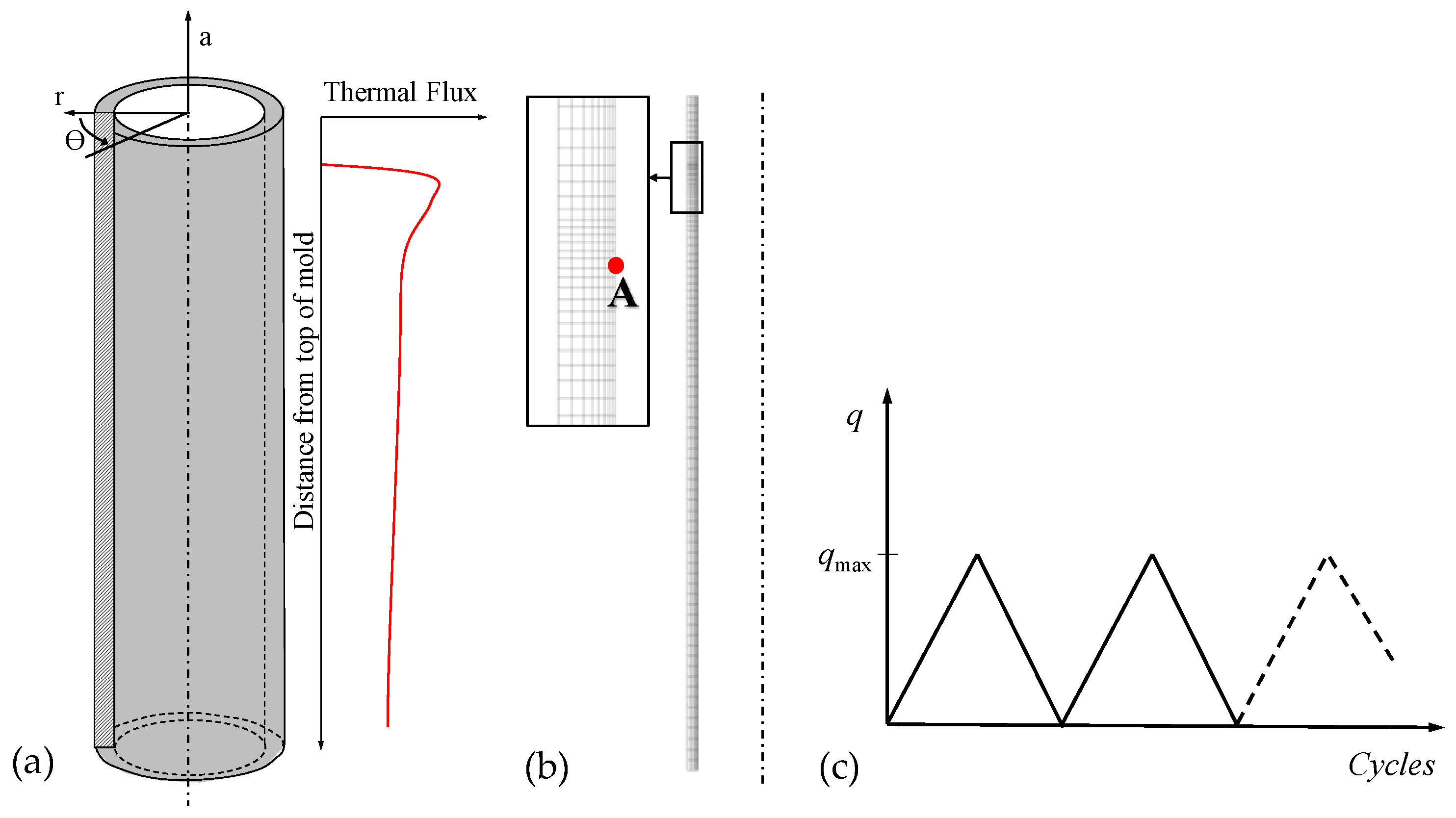
Metals 10 00781 g002
Figure 3. (a) Round mold with thermal flux distribution; (b) axisymmetric finite element (FE) model with mesh; (c) loading condition.
Metals 10 00781 g003
Figure 4. Combined material model for the round mold: (a) maximum stresses and (b) strain ranges, versus the number of cycles (point “A”; see Figure 3b).
Metals 10 00781 g004
Figure 5. Combined material model for the round mold: hoop stress–strain evolution (for more clarity, only some cycles are plotted).
Metals 10 00781 g005
Figure 6. (a) Cruciform welded joint; (b) finite element model with detailed mesh view of the weld toe and weld root; (c) loading condition; reproduced from [30] with permission from Elsevier, 2020.
Metals 10 00781 g006
Figure 7. Combined material model for the cruciform welded joint: (a) maximum stresses and (b) strain ranges, versus the number of cycles.
Metals 10 00781 g007
Figure 8. Stress–strain cycles in the x-direction with the combined material model; reproduced from [30] with permission from Elsevier, 2020.
Metals 10 00781 g008
Figure 9. Relative errors ∆e calculated with Equation (9) for nonlinear kinematic model calibrated on initial (E, σ0) and stabilized (Es, σ0*) static parameters: (a) mold (∆e < 0) and (b) cruciform joint (∆e > 0).
Metals 10 00781 g009
Figure 10. Equivalent strain range versus number of cycles (a) and relative errors ∆e calculated with Equation (9) by considering different accelerated models ba (b) for the round mold.
Metals 10 00781 g010
Figure 11. Equivalent strain range versus number of cycles (a) and relative errors ∆e calculated with Equation (9), considering different accelerated models ba (b) for the cruciform weld case study.
Metals 10 00781 g011
Figure 12. Correlation between speed of stabilization and number of cycles to stabilization for the mold and the welded joint.
Metals 10 00781 g012
Figure 13. Cyclic softening material behavior: evolution of the equivalent strain range and fatigue life assessment on a strain–life curve.
Metals 10 00781 g013
Figure 14. Cyclic hardening material behavior: evolution of the equivalent strain range and fatigue life assessment on a strain–life curve.
Metals 10 00781 g014
Figure 15. (a) Design diagram for mold T = 250 °C and cyclic softening material behavior; (b) schematic design diagram description
Metals 10 00781 g015
Figure 16. Schematic design diagram for a material with cyclic hardening behavior.
Metals 10 00781 g016
Table 1. Mechanical properties of CuAg0.1 alloy, data from [8].
Temp. (°C)E (MPa)Es (MPa)σ0 (MPa)σ0* (MPa)C (MPa)γR (MPa)b
20119,988114,7631138651,140702.4−682.352
250106,60094,7591105740,060915.8−753.894
300103,80094,7931085032,660737.3−775.293
Table 2. Cruciform welded joint: material parameters, data from [21].
MaterialE (MPa)σ0 (MPa)C (MPa)γR (MPa)b
Base metal SBHS500-2200,000452190361434
HAZ200,000542190361434
Weld metal200,000328215921131
Table 3. Number of cycles to stabilization and equivalent strain range estimated at the critical point.
Parameter MoldCruciform Joint
Reference ModelNonlinear KinematicReference ModelNonlinear Kinematic
InitialStabilizedInitialStabilized
Nstab48913137571010
Δεeq,stab0.00400.00340.00370.01990.10230.0201
Δe (%) −15.20−8.53 415.211.13
Table 4. Number of cycles to stabilization and equivalent strain range estimated at critical point “A”.
ParameterReference ModelAccelerated Models
10b20b30b100b200b300b421b
Nstab489713024108310
Δεeq,stab0.00400.0040 *0.0040 *0.0040 *0.0040 *0.0040 *0.0040 *0.0040 *
∆e (%) 0.490.470.410.120.15−0.53−0.83
* Rounded values.
Table 5. Number of cycles to stabilization and equivalent strain range for the critical point.
ParameterP100-U25 aReference ModelAccelerated Models
5b10b20b50b100b150b1500b2500b5000b
Nstab 757268193122119110113111113113
Δεeq,notch,stab0.01960.0199 *0.0197 *0.0196 *0.0196 *0.0195 *0.0195 *0.0195 *0.0195 *0.0195 *0.0195 *
Δe (%) 1.44 b−0.86−1.28 c−1.32 c−1.59 c−1.55 c−1.56 c−1.60 c−1.59 c−1.59 c
a [21]. b Relative difference calculated with respect to P100–U25. c Relative difference calculated with respect to the reference model. * Rounded values.
Table 6. Number of cycles to failure.
ParameterMoldCruciform Joint
Reference ModelNonlinear KinematicAccelerated Model 20bReference ModelNonlinear KinematicAccelerated Model 20b
InitialStabilizedInitialStabilized
Δεeq,stab0.00400.00340.00370.0040 *0.01990.10230.02010.0196
N27173786325126961235711961296
Relative error (%) 39.319.6−0.8 −99.4−3.24.9.
* Rounded value.

