A Modular Machine-Learning-Based Approach to Improve Tensile Properties Uniformity Along Hot Dip Galvanized Steel Strips for Automotive Applications

Abstract

The paper presents a machine learning-based system aimed at improving the homogeneity of tensile properties of steel strips for automotive applications over their strip length in the annealing and hot dip galvanizing lines. A novel modular approach is proposed exploiting process and product data and combining smart data pre-processing and cleansing algorithms, an ensemble of neural networks targeted to specific product classes and an ad-hoc developed iterative procedure for identifying the variability ranges of the most relevant process variables. A decision support concept is implemented through a software tool, which facilitates exploitation by plant managers and operators. The system has been tested on site. The results show its effectiveness in improving the control of the thermal evolution of the strip with respect to the standard operating practice.

1. Introduction

The European steel sector is investing incredible efforts for improving product quality in order to enforce its leadership and preserve its competitiveness on the global market. On the other hand, an ever increasing demand from customers is observed related to smaller and narrower tolerance ranges for significant quality attributes and material properties, which represents a relevant challenge for steel producers. For flat cold rolled steel products, which are devoted to demanding applications, such as the ones related to the automotive sector, one of the key features is represented by the mechanical properties. Therefore, the possibility to adjust and control product mechanical properties is crucial in order to reduce costs and improve revenues by reducing scrap and rate of downgraded coils.

Machine Learning (ML) is being intensively applied for on-line prediction and monitoring of mechanical properties of flat steel products. For instance, Lalam et al. in [1] apply a feed-forward Neural Network (NN) for the prediction of the mechanical properties of a coil from its chemical composition, thickness, width and key parameters related to the galvanizing process. On the other hand, Orta et al. in [2] propose a combination of analytical models and NNs in order to predict yield strength, tensile strength and elongation of cold rolled and continuous annealed steel grades, proving that NNs can enhance traditional models by capturing the highly non-linear relationships between mechanical properties and process parameters such as cold rolling reduction rate, annealing time, annealing temperature and contents of alloying elements. A further exemplar application of combined physically- and NN-based models can be found in [3] to the aim of predicting microstructure, average grain size and grain size distribution for cold-rolled and annealed austenitic stainless steels, which are fundamental in determining the product mechanical properties. A further paradigm for integration of physical modelling and ML techniques for mechanical properties prediction in cold rolled flat steel products is represented by the exploitation of ML tools for the identification of the parameters of complex analytical models. For instance, in [4] physically-based models for the prediction of tensile properties (Ultimate Tensile Strength and Yield Strength) of cold rolled Al-Killed and Interstitial Free (IF) steels are tuned through Genetic Algorithms (GA). In [5] data-driven models are developed for Ultimate Tensile Strength and percentage elongation, to the aim of achieving an optimum strength-ductility balance in Dual Phase (DP) and IF steels by optimizing the annealing cycle parameters through a multi-objective GA-based approach.

The considerable efforts of the steel sector toward digitalization, which are deeply analyzed in [6], allow foreseeing an increasing availability of process and product data from each stage of the process, including cold rolling and Hot Dip Galvanizing (HDG) lines, which will pave the way to an extensive profitable exploitation of ML-based tools for monitoring and forecasting of products mechanical properties. On the other hand, the possibility to include material property prediction in the process control loop either in the automation or, at least, through a decision support system guiding the operators in the setup of the process parameters, represents by itself a clear advance with respect to most currently existing systems. Such capability is, however, of poor practical advantage, if limited to a narrow category of known products for each single steelworks, without the possibility of adaptation to both the changing features of the plant and the evolution of the production. Moreover, so far most the developed applications are devoted to the achievement of a target average value of the mechanical properties, by neglecting the major problem of achieving uniformity of such mechanical properties along the coil.

Mechanical properties uniformity is actually a very relevant issue, such as extensively discussed by Van Den Berg et al. [7]. This paper is extracted from a project funded by the European Union, which deals exactly with product uniformity control. Lack of mechanical properties uniformity along the coil is actually a major cause of complaints from the customers. Being so important, the issue of uniformity has been investigated from the microstructure point of view in both hot and cold rolling. For instance, Li et al. in [8] aim at improving the longitudinal performance uniformity of hot-rolled coils by investigating through thermal simulation and hot rolling experiments the dynamic continuous cooling transformation, the influence of the cooling mode before coiling as well as the effect of the cooling rate during coil cooling on both microstructure and mechanical properties. A further example is provided by Goli-Oglu ena Efron, who investigate the effect of temperature regimes for accelerated cooling in the range 820–590 °C on low-carbon microalloyed steel plate microstructure and properties [9].

During cold rolling and HDG of flat steel products, tensile properties are usually assessed through mechanical tests on samples taken in different parts of the coils. Such properties are affected by the thermal evolution of the strip. From the process management point of view, plant operators tend to control the thermal path of the product mainly by acting on the reheating temperatures (reheating and soaking temperatures) and skinpass/tension leveller elongations, which surely impact but do not fully determine the thermal history of the product.

On the other hand, in cold rolling and HDG lines the tensile properties are continuously estimated with sophisticated online measurement systems. In particular, as far as flat products are concerned, two common commercially available online measuring systems for material properties are nowadays quite widespread in many the rolling mills: the Impulse Magnetic Process Online Controller (IMPOC) [7,10] and the Harmonic Analysis Coil Online Measurement System (HACOM) [11]. However, the obtained tensile properties measurements are not immediately exploitable in order to improve the process, as they are not fed back to the automation.

The overall aim of the work described in this paper is to achieve homogeneity of tensile properties over the coil length in annealing and HDG lines. To this aim, an advisory system is discussed, which supports the technical personnel in keeping the most relevant process variables within suitable ranges in order to limit the variability of the tensile properties along the coils. The system relies on ML for the preliminary analysis and cleansing of the raw data coming from the process as well as for the design and tuning of the models for materials properties prediction. Moreover, a specific iterative procedure is proposed, which exploits the models in order to determine the variability ranges for the process variables that mostly affect the mechanical properties.

Noticeably, the proposed concept does not affect the average values of the mechanical properties, which is supposed to be adequately addressed by the available process control system and operating practice of the personnel. In other words, the developed system mostly aims at ensuring that the possible variations of the tensile properties along the coil are limited, in order to avoid customers’ complaints. This represents a differentiating feature from previously developed approaches. Further elements of novelty are represented by a modular structure combining many “specialized” ML-based models of limited complexity, each targeting a specific product class, which can be individually designed and tuned according to the availability of historical data in sufficient number and quality.

The paper is organized as follows: Section 2 describes the considered industrial process and steel grades, the exploited process data as well as the methodological approach followed in the pre-elaboration of such data for models design and tuning. Section 3 is devoted to the decision-support concept, namely to the procedure for identification of the variability ranges for the process variables. Section 4 discusses the results of the tests developed by the company, which demonstrate the effectiveness of the proposed approach. Section 5 describes the software tool implementing the developed system to be used by plant operators. Finally, in Section 6, some concluding remarks and hints for future evolution of the proposed system are provided.

2. Materials and Methods

2.1. Industrial Layout

In the considered industrial plant, the cold rolled strips, rolled up as coils, coming from the pickling and cold rolling mill plants, are processed through a HDG process to cover them with a zinc coating, which prevents oxidation and corrosion phenomena. The considered HDG line processes cold rolled coils with a thickness in the range 0.4–2.5 mm and a width in the range 900–1950 mm, covering a wide range of steel qualities, from common Carbon steel to Advanced High Strength Steel (AHSS). The presented research work focuses on three steel grades covering the majority of the products of the concerned HDG line, which in the paper are indicated with the letters A, B and C.

The schematic layout of the considered HDG line is depicted in Figure 1.

In the considered process, a thermal treatment is performed by passing the strip through a vertical annealing furnace, composed of heating, soaking and rapid cooling sections. After the annealing process, the strip travels through a furnace snout and is then dipped into a bath of molten zinc at a temperature of about 460 °C. The zinc thickness is tightly controlled by an air knife system when the strip exits from the zinc pot. Subsequently, the strip is cooled down passing through a cooling tower, where air cooling is performed by fans coolers in both the ascending and descending parts. Afterwards, a final water quenching is executed in order to accelerate the cooling process. After being properly cooled, the strip is skin-passed and tension-levelled to improve the strip mechanical properties, surface quality and flatness.

The data that are collected along the above-depicted line and are exploited in the present work concern process parameters and steel chemical composition. Moreover, in the considered line, the mechanical properties (tensile strength, yield point) of each steel coil are continuously measured by means of an IMPOC [10]. IMPOC is an online material properties measurement system produced by EMG Automation GmbH (Wenden, Germany), which allows automatic non–destructive testing of ferromagnetic steel strips. The instrument systematically magnetizes the steel strip and measures the residual magnetic field. Based on mathematical models the mechanical properties tensile strength and yield point are calculated online along the length of the coil. The IMPOC measurements as well as the process variables are associated to longitudinal positions on the coil with a spatial interval ΔL = 10 m. The considered process parameters can be classified into the following categories:

• Temperatures measured in different zones i.e., the exit of heating/soaking sections of the Radiant Tube Furnace (RTF), the zones before and after the zinc bath, the top-roll cooling tower, the cooling water bath;
• Cooling devices, e.g., Fan Coolers (FC) along the cooling tower
• Skinpass Mill (SPM) (elongation, force …);
• Tension Leveller (TLV) (elongation, roll positions).

Table 1. List of considered process parameters for HDG line.

Symbol	Process Parameter
$x_1$	Exit heating Radiant Tube Furnace (RTF) strip Temperature
$x_2$	Exit soaking RTF strip Temperature
$x_3$	Deflector Roll 3 Temperature
$x_4$	Fans speed reference Rapid Cooling (RC) zone 1
$x_5$	Fans speed reference Rapid Cooling (RC) zone 2
$x_6$	Fans speed reference Rapid Cooling (RC) zone 3
$x_7$	Exit RC strip temperature
$x_8$	Deflector Roll 4 Temperature
$x_9$	Deflector Roll 5 Temperature
$x_{10}$	Tunnel zone Temperature
$x_{11}$	Hot Briddle Zone Temperature
$x_{12}$	Mobile Cooler (MC) cooling position
$x_{13}$	Mobile Cooler (MC) fans reference speed
$x_{14}$	Mobile Cooler (MC) fans reference speed zone 1
$x_{15}$	Mobile Cooler (MC) fans reference speed zone 2
$x_{16}$	Mobile Cooler (MC) fans reference speed zone 3
$x_{17}$	Mobile Cooler (MC) fans reference speed zone 4
$x_{18}$	Top Roll zone Temperature
$x_{19}$	Zone 1 Fan Coolers (FC) status
$x_{20}$	Zone 2 FC status
$x_{21}$	Zone 3 FC status
$x_{22}$	Temperature water bath cooling
$x_{23}$	Preset Skinpass Mill (SPM) elongation
$x_{24}$	Work Roll Diameter SPM
$x_{25}$	SPM Mode
$x_{26}$	SPM Emulsion
$x_{27}$	SPM Cleaning
$x_{28}$	Elongation SPM
$x_{29}$	Total Force SPM
$x_{30}$	Total Bending Force SPM
$x_{31}$	Entry Roll. Pos SPM (anty crimping)
$x_{32}$	Entry Roll. Pos SPM (billy-roll)
$x_{33}$	Preset Elongation Tension Leveller (TLV)
$x_{34}$	TLV use
$x_{35}$	Penetration Roll TLV N.1
$x_{36}$	Position Roll TLV anti-crossbow
$x_{37}$	Elongation TLV

lists all the considered 37 process parameters for the HDG line, while

Table 2. List of considered thickness ranges.

Thickness Range No.	Minimum Thickness (μm)	Maximum Thickness (μm)
1	500	700
2	700	900
3	900	1100
4	1100	1300
5	1300	1500
6	1500	1700
7	1700	1900
8	1900	2100
9	2100	2300
10	2300	2500

lists the 10 considered thickness ranges.

2.2. Data Pre Processing

In many ML applications, data pre-processing and filtering is needed in order to remove unnecessary samples and to obtain a dataset, which contains only reliable and plausible data correctly and fully representing the considered process. The importance of data pre-processing for the successful application of ML methods is extensively emphasized in literature, especially when dealing with industrial datasets [12,13,14,15]. Such preprocessing stages usually eliminate abnormal or unreliable data, the so-called outliers, and identify the variables, which mostly affect the target output of the models to design, by means of the so-called “variable selection” procedures. It must be underlined that a preliminary correlation analysis highlighted that the considered mechanical properties (Tensile Strength R_m and Yield Stress R_p0.2) are linearly correlated (correlation index r ≈ 0.99). This means, in practice, that we can focus on one of these properties and if this property is kept uniform, such uniformity holds also for the other one. Therefore, in the present application the target is the “Tensile Strength” (R_m).

In the considered application, process and product data, which had been collected for the design and implementation of the models predicting the product mechanical properties, have been, firstly, organized into a suitable dataset and, afterwards, treated though pre-processing and filtering procedures that allow obtaining a plausible and reliable dataset. Finally, the models input variables have been identified among all the measured parameters. In the present section, the applied pre-processing stages are described in detail.

The plausibility analysis includes both the definition of a plausibility range for each process variable, according to the suggestion of the technical personnel of the steelworks, and the elimination of the variables associated to more than 30% of not plausible measurements.

The outlier detection analysis exploits a fuzzy logic-based procedure, which combines four traditional approaches through a Fuzzy Inference System (FIS) [16]. For each data sample, four features are extracted by exploiting traditional methods for outliers identification [17,18,19,20,21]. Such features are based on the most widely adopted definitions of outlier, which can be found in literature. The exploited indexes quantify for each sample: (i) the “distance” from the rest of the data [22]; (ii) the “position” with respect to the statistical distribution of the dataset [23]; (iii) the density of the rest of the data in the surroundings [24]; (iv) the degree of membership to the different clusters, in which the dataset can be grouped via the fuzzy c-means clustering [25]. The four features are fed as inputs to the FIS that provides as output an outlier degree to be compared with a predetermined threshold in order to assess if the sample is an outlier. The advantage of the adopted FIS-based approach with respect to traditional approaches lies in the possibility of jointly exploiting the advantages of the combined traditional methods while overcoming their complementary limitations. A further important advantage of the proposed outlier detection approach lies in the fact that this algorithm is fully automatic and does not require any a priori information on the processed dataset, as all required parameters for the elaboration (e.g., the number of clusters for the clustering algorithm) are automatically evaluated. These aspects ensure good performances on databases with very different features, by thus facilitating the deploying of the system in the industrial contexts.

Once abnormal data are eliminated (in the present case they represented about 30% of the whole data set), a preliminary rough elimination of markedly irrelevant variables has been performed by exploiting the domain knowledge of technical personnel of the company. Nonetheless, the number of available potential input variables of the models to develop remains huge. Therefore, a further stage for dimensional data reduction is needed. Such stage transforms a wide dataset into a smaller one by retaining most of the relevant information content of the original dataset. Dimensional data reduction is performed through the following two main steps.

• Removal of highly correlated variables in order to eliminate redundancy in the dataset (also called “redundancy analysis”);
• Selection of the variables which mostly affect the product mechanical characteristics (i.e., “variable selection”).

The selection of the best subset of informative and uncorrelated variables helps the minimization of models prediction error.

The redundancy analysis has been performed by applying the “dominating set algorithm”, a procedure derived from graph theory [26,27]. The dominating set algorithm identifies the highly correlated variables through the definition of a sort of graph where the vertexes correspond to the variables: two vertices are linked when the corresponding couple of variables show a high linear correlation. The minimum dominating set of the constructed graph is the subset of vertices such that every vertex, which is not included in it, is linked to a vertex of the dominating set. A variable is redundant if the corresponding vertex of the graph is not included in the minimum dominating set. The dominating set algorithm is computationally expensive, like many other computationally hard graph theoretic problems [28], but a suboptimal solution can be obtained in reasonable time.

The variable selection has been performed by exploiting a procedure [29] based on a Genetic Algorithm (GA). In synthesis, within such procedure, each variable subset is represented through a binary chromosome of the GA, i.e., each gene is univocally associated to an input variable and is unitary, if the corresponding variable is included in the considered subset, null otherwise. The GA generates a so-called “population” of different chromosomes, i.e., potential variables subsets, and evaluates their goodness according to a so-called “fitness function”, which is related to the model performance when trained by exploiting the corresponding input variable subset. The best chromosomes are used (by duplicating, mating or mutating them according to the GA crossover and mutation procedures) to generate a new population. In particular, the crossover operator creates the son chromosome by randomly capturing the genes values from the two parents, while the mutation operation generates new individuals by randomly selecting a gene of one chromosome and switching it from 1 to 0 or vice-versa. Once a new population is built, the evaluation and reproduction process is iterated until a stop condition is reached. In the present case, the stop condition consists in the achievement of either a fixed number of iterations or a plateau for the fitness function. The above-described GA-based procedure, which was proposed by the authors, already proved to be effective in a number of industrial applications and with different kinds of ML-based models (see, for instance, an application to Echo State NNs in [30]) both in terms of efficient identification of the most relevant variables and in terms of “stability”. The stability is defined as the sensitivity of a variable selection algorithm with respect to variations in dataset that is used for model parameters tuning and is a very relevant property especially when dealing with ML-based models. In practice, a variable selection procedure is unstable when, for the same problem, the adoption of different training sets for the model tuning procedure leads to the selection of different variable subsets.

2.3. Data-Driven Models Identification Procedure

For the purpose of the models development, the pursued approach focuses on the definition and tuning of a series of simple models estimating the R_m value of the final product, which are specialised for a narrow range of product variables. In particular, as steel grade and product thickness have been recognised as very significant aspects affecting R_m, coils have been grouped on the basis of the steel grade and each group has been further divided in 10 different classes corresponding to different and not overlapping thickness ranges. Therefore, in this study, a total number of 30 models have been designed and their parameters identified.

For each sub-model, two simple kinds of models for mechanical properties prediction have been tested: a first-order polynomial model and Feed-Forward Neural Networks (FFNN) of the Multi-Layer Perceptron type [31] with two hidden layers with sigmoidal activation function and a linear output layer. The linear models have been identified with the standard pseudo-inversion procedure [32]. For the FFNN-based models, the number of neurons in the hidden layers of the models is empirically calculated and the internal model parameters are identified by means of the standard backpropagation algorithm [33]. Such number can be generally different for each model, also depending on the number of available data, but it is generally limited. For instance, with the available initial database, a few hidden neurons (from 2 to 5) are sufficient. The FFNN-based models show a stable behavior, while some problems of instability can arise for linear models due to the possibility to have a singularity of the data matrix.

3. The Decision Support Concept

The objective of the decision support concept is to find appropriate bounds for the relevant process variables such that the predicted value of R_m lies in a controlled and limited range throughout the whole length of the coil, in order to ensure the uniformity of such mechanical property. All the process variables, which are considered as potential inputs for the models, lie in a limited range $\left[l{b}_i,u{b}_i\right]$ for $1\le i\le 37$ where $l{b}_i$ and $u{b}_i$ are, respectively, the lower and upper bounds for the i-th variable. Some of these bounds are identified by exploiting knowledge domain, while other ones are set by simply considering the minimum and maximum value assumed by the corresponding variable within the available dataset. The main idea behind the decision support concept is to use the previously trained models as a “soft sensor” providing the R_m value at each point of the coil based on some process variables. Such variables cannot be kept perfectly constant through time and their values can vary even during the time required for processing one coil. However, based on the models, R_m can be estimated for any possible combination of such variables, and, thus, the range of variability can be determined for the estimated R_m, when the model input variables lie in predetermined intervals. Lack of uniformity means that such range is too wide and, in order to keep uniformity, the ranges of variation of the input variables need to be somehow “shrunk.” The decision support concept identifies the maximum ranges within which the process variables can vary in order to ensure that the variation range of R_m along the coil is compatible with a predefined requirement, so as to be considered uniform. The same approach can also be extended to ensure the intra-coil uniformity, namely to ensure that the R_m value does not sensibly vary among different subsequent coils belonging to the same steel grade and thickness range.

Please note that the proposed concept does not affect the average value of R_m, i.e., is not aimed at ensuring that R_m lies in a range centered on a given value, but only that the possible variations of its value along the coil are lower than a threshold value named “Uniformity Threshold” (UT). In order to take into account the prediction error of the models, for each steel grade and each thickness value, UT is computed as the difference between a maximum allowed variation provided by the technical personnel of the HDG line and the mean absolute prediction error, which characterizes each model and is computed during its identification procedure.

Let us indicate with the symbols $\mathit{L}$ and $\mathit{U}$ two “bound vectors” defining the lower and upper limit for the input variables of each model adopted for the estimate of R_m. The decision support concept is based on a recursive adaptation of such vectors. A standard nonlinear optimization algorithm falling in the class of interior-point methods is exploited [34], which performs a constrained optimization on the function represented by one of the previously trained models, and allows calculating the minimum and maximum values $m\left(\mathit{L},\mathit{U}\right)$ and $M\left(\mathit{L},\mathit{U}\right)$ of R_m, which are assumed when the model input variables lie in the ranges identified by $\mathit{L}$ and $\mathit{U}$. The maximum predicted range of variation of R_m is defined as:

$$d\left(\mathit{L},\mathit{U}\right)≔M\left(\mathit{L},\mathit{U}\right)-m\left(\mathit{L},\mathit{U}\right)$$

(1)

In other words, $d\left(\mathit{L},\mathit{U}\right)$ identifies the forecasted range of variability of R_m when the process variables lie in the ranges defined by $\mathit{L}$ and $\mathit{U}$. If such range is suitable for the analyzed steel grade and thickness, namely if $d\left(\mathit{L},\mathit{U}\right)\le UT$ for the considered product, then the lower and upper bounds are feasible. Otherwise the bounds $\mathit{L}$ and $\mathit{U}$ are recursively modified in order to narrow the range of variability of the process variables until $d\left(\mathit{L},\mathit{U}\right)$ achieves a suitable value. Clearly the entries of $\mathit{L}$ and $\mathit{U}$ initially coincide, respectively, with the lower bounds $l{b}_i$ and upper bounds $u{b}_i$ of the considered process variables.

The implemented recursive algorithm requires the preliminary estimate of some coefficients, which are extracted from the trained models. Firstly, the parameters ${\sigma }_i^{+}$ and ${\sigma }_i^{-}$ are computed, which measure the “positive” and “negative sensitivity” of the R_m estimate with respect to the variable $x_i$. Such parameters are computed by performing a sensitivity analysis procedure that evaluates the approximated partial derivatives of every variable in a number of “key points”. The values of the partial derivatives of a real-valued function $y=f\left(\mathit{X}\right)$ defined on a domain $\mathcal{D}\subseteq {ℝ}^n$ in a generic point $\overline{\mathit{X}}\in \mathcal{D}$ represent reasonable measures of the correlation between each entry of the vector $\mathit{X}$ and the independent variable $y$ in a neighborhood of the point $\overline{\mathit{X}}$. Therefore, the mean value of such partial derivatives computed over some key points can provide an acceptable measure of the global correlations between each entry of $\mathit{X}$ and $y$. In the present case, the considered real-valued function is the model forecasting R_m for the considered steel code and thickness range as a function of its input variables. As far as the selection of the key points is concerned, our approach consists in randomly selecting the key points within the domains $\mathcal{D}$ of the model, which is an hypercube contained in ${ℝ}^P$, being P the number of input variables selected for each model (as each variable lies in the interval comprised between the upper and lower bounds). The number of the considered key points needs to be high (e.g., 100) in order to enhance the probability of suitably covering the considered domain. Let us consider for one single model with $P$ input variables ($1\le P\le 37$) the key point $\overline{\mathit{X}}=\left(\overline{X_1},\dots ,\overline{X_i},\dots ,\overline{X_P}\right)$. The partial derivatives of R_m with respect to the i-th variable in such key point are estimated by varying only the entry $\overline{X_i}$ on a regular grid of N equidistant values lying in the range $\left[l{b}_i, u{b}_i\right]$. The computed N values of the partial differential ratio are split into two subsets containing, respectively, the negative and positive values. The average values ${\mathsf{\Sigma }}_i^{-}$ and ${\mathsf{\Sigma }}_i^{+}$ of such two subsets are then normalized and tightened in order to extract the parameters ${\sigma }_i^{-}$ and ${\sigma }_i^{+}$.

Moreover, in order to implement the recursive algorithm, two further auxiliary vectors named $\mathit{L}\prime$ and $\mathit{U}\prime$ are calculated so that $\forall i, 1\le i\le 37$ $L{\prime }_i\ge l{b}_i$ and $U{\prime }_i\le u{b}_i$. If no technical constraints or user’s specifications on the variable range is available, each entry of $\mathit{L}\prime$ and $\mathit{U}\prime$ is computed from the available historical data such that for all $i, 1\le i\le 37$ the relationships $x_i<L{\prime }_i$ and $x_i>U{\prime }_i$ hold for the 40% of the available field data. These vectors represent a sort of “safety variability ranges” for the variable. In effects, due to the data-driven nature of the models and the fact that many data used for their training correspond to uniform products, when $L{\prime }_i\le x_i\le U{\prime }_i$ for all their input variables, the variability range of R_m is compliant with the requirement of uniformity.

To sum up, once the steel grade and the thickness value are fixed, and consequently, the model is identified, which requires as input a subset $\mathcal{A}$ of the 37 process variables, the iterative procedure works as follows. Initially, i.e., at step $k=0$, the bound vectors ${\mathit{L}}^{\left(0\right)}$ and ${\mathit{U}}^{\left(0\right)}$ are built by using as entries the lower bounds $l{b}_i$ and upper bounds $u{b}_i$ of the $P$ process variables, which must be fed as inputs to the considered model. The variability range $d\left({\mathit{L}}^{\left(0\right)},{\mathit{U}}^{\left(0\right)}\right)$ for R_m is estimated by running the constrained optimization algorithm and is compared to the UT value for the considered steel grade and thickness range. If $d\left({\mathit{L}}^{\left(0\right)},{\mathit{U}}^{\left(0\right)}\right)>UT$, the bound vectors are modified. At the generic k-th step of the recursive algorithm, the entries of the vectors ${\mathit{L}}^{\left(k\right)}$ and ${\mathit{U}}^{\left(k\right)}$ are modified as follows:

$$L_i^{\left(k\right)}=\min \left\{L_i^{\left(k-1\right)}+\left(U_i^{\left(k-1\right)}-L_i^{\left(k-1\right)}\right)·{\sigma }_i^{+},L{\prime }_i \right\} \forall i:x_i\in \mathcal{A}$$

(2)

$$U_i^{\left(k\right)}=\max \left\{U_i^{\left(k-1\right)}+\left(U_i^{\left(k-1\right)}-L_i^{\left(k-1\right)}\right)·{\sigma }_i^{-}, U{\prime }_i\right\} \forall i:x_i\in \mathcal{A}$$

(3)

Clearly, if the measure of the negative correlation ${\sigma }_i^{-}$ is null, then lower bound of the i-th variable remains constant at each iteration and, similarly if ${\sigma }_i^{+}$ is null, then Equation (3) does not vary the value of the upper bound at each iteration. The variability range of R_m at step $d\left({\mathit{L}}^{\left(k\right)},{\mathit{U}}^{\left(k\right)}\right)$ is computed and compared to UT. The algorithm terminates when $d\left({\mathit{L}}^{\left(k\right)},{\mathit{U}}^{\left(k\right)}\right)<UT$ or when $\forall i:x_i\in \mathcal{A}$ $L_i^{\left(k\right)}=L{\prime }_i$ and $U_i^{\left(k\right)}=U{\prime }_i$. The final bounds are used in the decision support system. A schematic presentation of the proposed algorithm, which is named L-U search, is shown in Figure 2.

Figure 3 summarizes the overall flow diagram of the proposed approach by depicting the link between data collection, pre-processing, model design and tuning and the decision support system: the database is initialized with a possibly incomplete set of historical data allowing the identification of the most relevant process variables as well as the design and identification of a set of models which can cover all or part of the product range. Once the variability ranges of the relevant process variables are determined through the L-U search, an advisory system provides suggestions to the operators by also facilitating process monitoring (more details will be provided in Section 5). During plant operations, new data are collected, which can be periodically exploited, after suitable pre-processing, in order to re-tune the existing models or redesign them or build further models covering products, which were not suitably represented within the initial database.

4. Numerical Results

The proposed approach has been tested on 3 different steel grades and 10 thickness ranges: therefore, in theory 30 FFNN-based models should have been designed and identified by exploiting field data. However, in order to obtain trustable models, a sufficient number of reliable data (i.e., data which underwent the pre-processing stage) need to be available. This was not possible for all the combinations of steel grade and thickness. For steel grade A, not enough data were available related to thickness range 9; for steel grade B, not enough data were available related to thickness ranges 1 and 9; for steel grade C, not enough data were available related to thickness ranges 1 and 5. Therefore, finally 25 models FFNN-based models have been designed and identified. As an example,

Table 3. Selected input variables for the models related to steel grade A for the thickness ranges with a sufficient number of data.

Thickness Range	Selected Variables
1	$x_1, x_2, x_3,x_5, x_6, x_7,x_8, x_9, x_{11},x_{12}, x_{13},x_{14}, x_{15},x_{17},x_{18},x_{23},x_{25},x_{28},x_{29},x_{30}, x_{33}$
2	$x_1, x_2, x_3,x_4, x_7,x_8, x_9, x_{10},x_{11}, x_{14}, x_{15},x_{17},x_{22},x_{23},x_{24},x_{25},x_{26},x_{28},x_{29}$
3	$x_1, x_2, x_5,x_8, x_9, x_{10},x_{11}, x_{13}, x_{15},x_{18},x_{22},x_{28},x_{30}$
4	$x_1, x_2, x_3,x_5, x_7,x_9, x_{11},x_{15},x_{17},x_{18},x_{24},x_{25},x_{26},x_{27},x_{28},x_{29}$
5	$x_1, x_2, x_3,x_4,x_5, x_{10}, x_{13},x_{17},x_{18},x_{22},x_{24},x_{27},x_{28},x_{29},x_{30}, x_{31}$
6	$x_1, x_2, x_4,x_5, x_7, x_9, x_{10},x_{11}, x_{13}, x_{15},x_{16},x_{17},x_{18},x_{26},x_{27},x_{28},x_{30}, x_{31}$
7	$x_1, x_2, x_5, x_8, x_9, x_{10},x_{11}, x_{13},x_{14}, x_{16},x_{18},x_{24},x_{25},x_{27},x_{28},x_{29},$
8	$x_2, x_3, x_9, x_{18},x_{23},x_{25},x_{26},x_{27},x_{28},x_{29},x_{31}, x_{33}$
10	$x_1, x_2, x_4, x_7, x_{15}, x_{16},x_{17},x_{28},x_{29},x_{30}, x_{33}, x_{37}$

reports the selected input variables for the models related to steel grade A for all the thickness ranges apart from the 9-th one. The computed values of the uniformity threshold TU for all the 25 models are reported in

Table 4. Values of the uniformity threshold UT for all the 25 FFNN-based models.

Thickness Range	TU (MPa)
	Steel Code A	Steel Code B	Steel Code C
1	14	-	-
2	12	33	21
3	11	31	31
4	12	26	30
5	14	33	-
6	10	35	29
7	12	25	32
8	13	34	16
9	-	-	29
10	5	33	26

.

For each steel code and thickness range, the variability ranges of the relevant process variables have been determined by means of the iterative procedure described in Section 3, which are reported for each steel grade in Figure A1, Figure A2 and Figure A3 of Appendix A.

The proposed decision support concept was tested on the field in the HDG line. In particular, two types of tests were performed to validate the proposed algorithm:

• Off-line test using an historical database related to previously produced coils, which were not considered in the design of the models and of the L-U search algorithm;
• On-line test, in which new coils have been manufactured according to the suggestions provided by the system.

In both cases, coil mechanical properties were measured through offline mechanical tests performed in the company’s laboratory in compliance with the UNI EN ISO 6892-1 norm on product samples taken on head, center and tail of each coil. In particular, three mechanical properties were considered in the test: the Yield Stress at 0.2% of elongation R_p0.2, the Tensile Strength R_m and the total percentage elongation of the specimen (gauge length: 80 mm) A_80mm%.

Moreover, the decision was taken to focus on a sub-set of parameters, i.e., reheating/soaking temperatures, fans speed reference zones in rapid cooling, MC fans speed reference in cooling tower, skinpass mode, skinpass working rolls diameter, tension leveller mode, tension leveller elongation. The rationale behind such choice lies is twofold: firstly, the selected parameters more heavily affect the heating pattern of the strip or the mechanical deformation during skinpass/tension leveller operations. Secondly, in the standard operating practice it is easier for the technical personnel to constrain the variability of the selected parameters and this facilitated the development of the on-line test and allowed the off-line test providing more realistic results.

In both tests, in order to evaluate the test results, the standard deviation of each mechanical property was computed on three different sets of coils: (i) all the considered coils; (ii) all the coils produced with reheating/soaking temperature lying in a predefined and recommended range (which is named “Reference Set”); (iii) only the coils produced according to the criteria suggested by the developed system (which is indicated as “Test Set”). The reason for introducing the second set consists in the fact that the reheating temperature T_RH is considered the main driving force to achieve the desired mechanical properties uniformity. Therefore, the “Reference Set” is considered a reliable term of comparison in order to assess the efficiency of the system in improving the control of the thermal evolution of the strip during the process with respect to the standard operating practice, which is based only on the control of the reheating temperature.

The offline test was performed by considering for steel codes A and C the thickness range 2 (0.7–0.9 mm) and for Steel Code B the thickness range 3 (0.9–1.1 mm). The selection of the thickness ranges was done considering the required parameters bounds and the number of available coils in the database. In particular, the test considered 3738 coils for Steel Code A, 1385 coils for Steel Code B and 1443 coils for Steel Code C. Among these coils, 1057 coils for Steel Code A were produced with a T_RH value lying in the range 820–830 °C, 382 coils for Steel Code B were produced with 810 °C ≤ T_RH ≤ 830 °C and 910 coils for Steel Code C were produced with 770 °C ≤ T_RH ≤790 °C. The numbers of coils, which were produced according to the criteria suggested by the developed system, are 147 for Steel Code A, 7 for Steel Code B and 17 for Steel Code C.

Table 5. Results of the offline tests for Steel Code A and thickness range 2 (0.7–0.9 mm).

Set	Rp0.2 (MPa)		Rm (MPa)		A80mm%
	Average	Std. Dev.	Average	Std. Dev.	Average	Std. Dev.
All Coils	168	12.5	295	8.5	40.8	2.0
Reference Set (820 °C ≤ TRH ≤ 830 °C)	164	10.4	295	8.4	40.9	1.8
Test Set	159	8.8	293	7.5	40.9	1.5

,

Table 6. Results of the offline tests for Steel Code B and thickness range 3 (0.9–1.1 mm).

Set	Rp0.2 (MPa)		Rm (MPa)		A80mm%
	Average	Std. Dev.	Average	Std. Dev.	Average	Std. Dev.
All Coils	307	26.0	383	16.0	31.5	2.7
Reference Set (810 °C ≤ TRH ≤ 830 °C)	309	20.8	377	10.0	32.8	1.6
Test Set	304	15.7	380	5.9	32.5	1.3

and

Table 7. Results of the offline tests for Steel Code C and thickness range 2 (0.7–0.9 mm).

Set	Rp0.2 (MPa)		Rm (MPa)		A80mm%
	Average	Std. Dev.	Average	Std. Dev.	Average	Std. Dev.
All Coils	371	28.9	460	24.7	26.1	3.3
Reference Set (770 °C ≤ TRH ≤ 790 °C)	372	27.2	457	22.2	26.4	3.3
Test Set	386	24.8	457	19.9	27.2	2.0

depict the results of the offline test for Steel Code A, B and C, respectively. For each considered mechanical property, the average value and the standard deviation (Std. Dev) on the three sets of coils are shown.

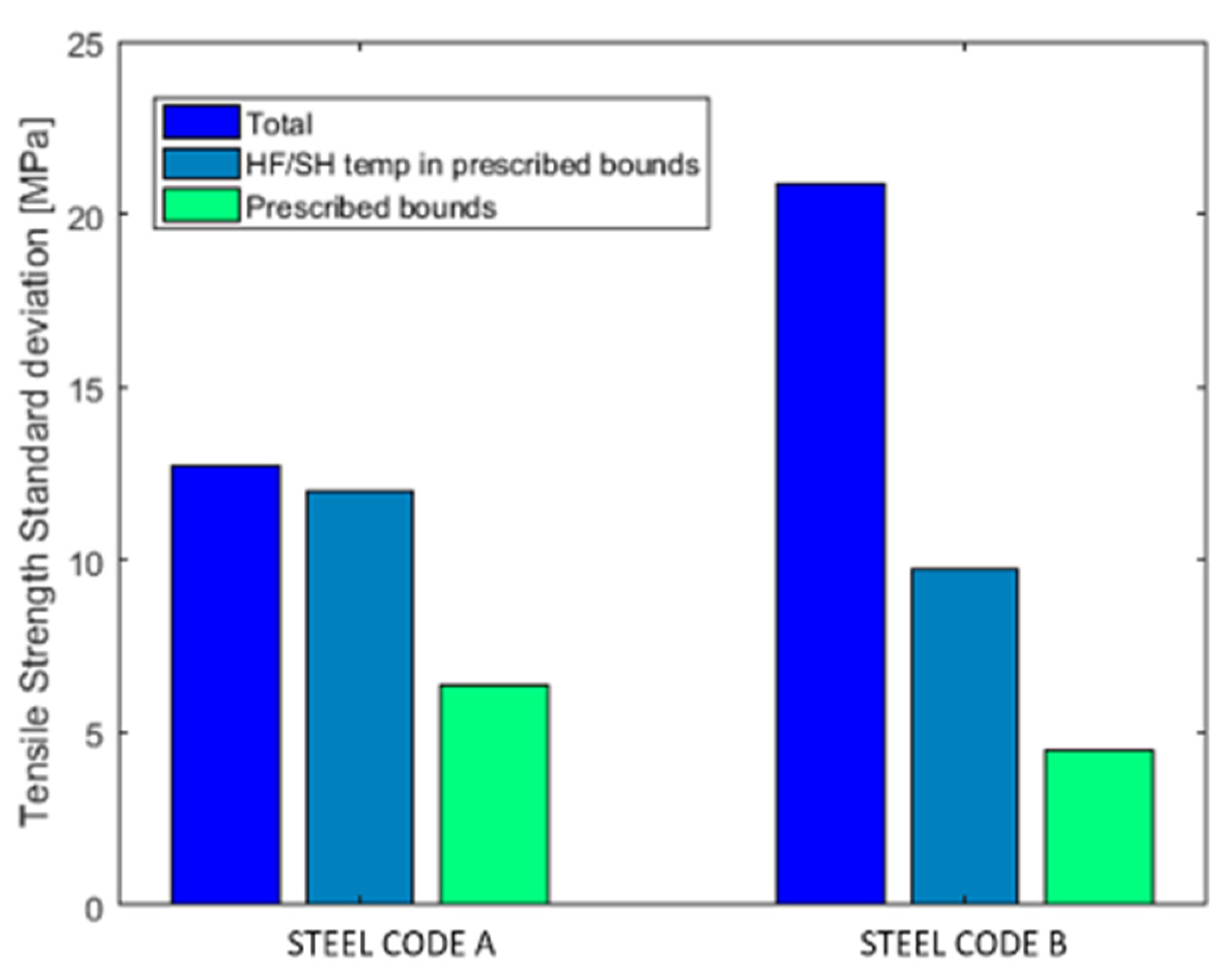
For Steel Code A, results show that keeping the heating Temperature within the recommended range helps reducing the variability of R_p0.2 and A_80mm%. On the other hand, keeping all the considered parameters within the bounds suggested by the developed system allows sensibly reducing the standard deviation of all the considered mechanical properties with respect to both the values referred to all the available coils and the values related to the Reference Set.

Steel Code B was less frequently produced with respect to Steel Code A in the period covered by the exploited historical database. The total number of coils is far lower than in the previous case and the number of coils produced keeping all the considered parameters within the bounds suggested by the developed system is very low. Therefore, it is not easy to draw reliable conclusions. Nevertheless, these results still confirm a relevant reduction of the standard deviation especially as far as R_p0.2 is concerned.

Compared with the previous two Steel Codes, the results for Steel Code C show higher standard deviation values for both the total production and the Reference Set. This phenomenon is mainly due to the supplying conditions of the coils (chemical composition and hot rolling parameters) and keeping T_RH within the recommended range does not reduce the variability of the mechanical properties. On the other hand, the coils produced according to the process parameters settings suggested by the developed system show a lower standard deviation of all the three considered mechanical properties.

Figure 4 summarizes the outcome of the offline test for all the three considered product classes as far as the standard deviation of R_m is concerned.

The on-line test was performed on steel codes A and B respectively on thickness range 2 (0.7–0.9 mm) and 3 (0.9–1.1 mm). Steel grade C was not taken into account, because it was not produced during the test period. Moreover, the above-mentioned thickness ranges have been selected considering the availability of existing order on the thickness classes, the availability of a restricted range on reheating temperatures and, finally, the availability of prescriptions on skinpass setting and cooling pattern. In particular, for Steel Code A, 13 coils coming from 7 different casts and, for Steel Code B, 4 coils coming from 2 different casts were specifically produced in two different campaigns according to the criteria suggested by the developed system. These coils represent the Test Set for the two considered Steel Codes. The Reference Set of coils produced in the same period is composed, for Steel Code A, by 81 coils coming from 46 casts produced with a reheating temperature 820 °C ≤ T_RH ≤ 830 °C, while for Steel Code B includes 6 coils coming from 6 different casts produced with 810 °C ≤ T_RH ≤ 830 °C. The total number of coils produced is 324 for Steel Code A and thickness range 2 and 38 for steel code B and thickness range 3.

Table 8. Results of the on-line tests for Steel Code A and thickness range 2 (0.7–0.9 mm).

Set	Rp0.2 (MPa)		Rm (MPa)		A80mm%
	Average	Std. Dev.	Average	Std. Dev.	Average	Std. Dev.
All Coils	167	20.2	300	12.7	39.8	2.3
Reference Set (820 °C ≤ TRH ≤ 830 °C)	163	15.3	297	12.0	40	3.4
Test Set	166	5.1	301	6.4	39.7	1.6

and

Table 9. Results of the on-line tests for Steel Code B and thickness range 3 (0.9–1.1 mm).

Set	Rp0.2 (MPa)		Rm (MPa)		A80mm%
	Average	Std. Dev.	Average	Std. Dev.	Average	Std. Dev.
All Coils	307	33.4	391	20.9	31.0	2.2
Reference Set (810 °C ≤ TRH ≤ 830 °C)	293	15.0	378	9.7	32.9	1.4
Test Set	295	8.3	381	4.5	32.7	0.6

depict the results of the on-line test for Steel Code A and Steel Code B.

The results of the on-line test show that the proposed approach allows decreasing the standard deviation of all the three considered mechanical properties for both classes of considered products. In other words, by keeping the considered process variables within the bounds suggested by the developed approach, the average values of all the three mechanical properties do not show relevant discrepancies, while their variability is drastically reduced also with respect to the case where the reheating temperature is kept within the suggested range. Figure 5 shows the decrease of the standard deviation of R_m for both the considered product classes. This confirms that the proposed approach improves the control of the thermal evolution of the strip.

To sum up, the onsite tests confirm and further demonstrate the efficiency of the proposed approach, which suggests process settings increasing the uniformity of mechanical properties along the coils. Both tests also confirm the strong link among the mechanical properties, also known form the basic metallurgy, which means that focusing on the improvement of the uniformity of one of them is beneficial for the uniformity of the other ones.

The combination of these data also allows the technical personnel better understanding the behavior of the material during the HDG process, by optimizing the parameters in order to obtain the required mechanical properties of the product.

5. The Developed Software Tool

In order to help the operators and plant managers to exploit at best the potential of the developed approach, a software tool has been developed, which both provides suggestion on parameters settings and allows exploiting historical data for the system fine tuning and performance improvement. The Unified Modelling Language (UML) diagram of main use cases of the developed software is shown in Figure 6.

The tool holds a component, which allows running the models identification procedure described in Section 2.3 and is linked to a products database, which is fed by plant data and is connected to the plant IT system. Such component comes equipped with a user-friendly interface, which holds some filter functionalities, such as steel quality selection, thickness range selection, coils production time range selection, mechanical property selection and prediction model type selection. The UML activity diagram related to the model identification use case is shown in Figure 7.

According to the specifications provided by the user, the data related to all coils of the selected steel quality and thickness range, which have been produced in the selected time period, are loaded from the database and joined into a dataset. Such dataset undergoes all the pre-processing stages, which are described in Section 2.2 by generating the input dataset for the selected model type. Figure 8 shows some exemplar screenshots of the user-friendly interface for data selection and models tuning. In particular, the window for the selection of the most appropriate process parameters to be fed as input for the selected model type is shown. Moreover, a diagram depicts the behavior of the selected model: the prediction performance of the model is characterized in terms of both prediction error and standard deviation on the considered dataset.

By exploiting this module, as soon as new data become available, the user can carry out a training procedure on each model in order to design a new model or increase the prediction accuracy of previously settled models. Clearly, the input dataset, which is used to re-tune a previously settled model is built by applying the same techniques for data pre-processing and filtering, but only data coming from reliable coils, which are identified by the pre-processing and filtering stage, are exploited. Moreover, a new test set (different from the training dataset) is built containing also newly acquired data, on which the re-tuned model is tested. After the FFNN-based model training, its performance is evaluated on the tests set and can be compared to the one of the “old” model. Based on such comparison, the user can decide whether to replace the old model with the new one.

A further software module has been developed in order to support the operators by detecting the recommended process parameters and their suggested bounds in order to ensure mechanical properties uniformity. Such module is equipped with a user-friendly graphical interface, which also allows visualizing the process parameters trends on coils selected by the user. Figure 9 shows the UML activities diagrams corresponding to the plant operator use cases related to the visualization of the suggested bounds for recommended parameters and of the process parameters trends, which are also compared to the bounds.

When started, such module shows a window where the user can select a steel code and a thickness range as well as the functionality to be executed (see Figure 10). By clicking on the “Lower/Upper Bounds” button, the suggested process parameters and their associated bounds can be visualized in a second window. Such window also allows visualizing all the available process parameters and, in this case, the suggested ones are marked as selected and highlighted with dark blue color, such as exemplarily depicted in Figure 10.

In addition, the module allows visualizing the process parameters trends for a set of coils selected by the user. When clicking on the button “Parameter trend overview”, a window is opened, which allows the user selecting a set of coils and a set of process parameters to be visualized and shows the values of the suggested bounds of each process variable. Moreover, a fixed production time period can be selected and all the coils produced in the selected period and belonging to the selected steel quality and thickness range, can be loaded in the coils view window sorted by ending production time. It is possible to select coils either jointly or individually. Subsequently, the user can select one or more process parameters among the suggested ones (for the selected steel quality and thickness range) or among all 37 considered parameters in order to visualize them and to compare their trends to the suggested bounds (when available), such as exemplary shown in Figure 11.

To sum up, this tool support the operators not only in the exploitation of the decision support concept developed within the project, but allows refining and improving its performance through time, according to the variable features of the production, as well as monitoring the process evolution, by also contributing to improve process overall monitoring and knowledge.

The developed tool is modular, according to the approach followed also for the system development and this feature represents an advantage in terms of flexibility and suitability for industrial deployment. In other words, the system can be started also with an incomplete dataset concerning coils, which does not fully cover the whole product range of the company. The system will begin providing trustable results and useful suggestions for the classes of products (i.e., steel codes and thickness ranges) for which a higher number of data is present in the available database. As soon as more (and/or better i.e., more reliable) data become available, new models can be designed to cover other products, while previously settled models can be refined in order to improve their performance. This feature allows the system gradually improving its reliability through time and being always updated with respect to the company’s production demands and features.

6. Conclusions

An effective approach for improving uniformity of mechanical properties along the steel coils produced in an HDG line is proposed, which exploits the available process data and the measurements provided by the IMPOC and suggests proper variability ranges for the variables, which are considered more relevant in the determination of the aimed uniformity for each product class. The proposed concept is data-driven and, therefore, relies on a comprehensive preliminary data pre-processing stage aimed at ensuring the quality of the data that are exploited to tune data-driven models forecasting the Ultimate Tensile Strength. Such models are exploited by an ad-hoc iterative procedure, the L-U search, which identifies the variability ranges of the relevant process variables. A software tool has also been developed, in order to provide the plant operators with an easy-to-use interface allowing full exploitation of the potential and features of the developed system.

The proposed decision support concept has been tested on the field through both off-line and on-line tests. The results of such tests highlight improved homogeneity in mechanical properties when using the recommended settings. Besides having targets on reheating temperature, more attention can be paid to variables related to intermediate cooling steps, such as hot bridle temperature (before the pot) and top roll temperature (after the pot). Data on cooling fans in rapid cooling and in mobile cooler have been adopted in order to properly set the cooling devices for achieving the desired temperatures. Data on skin pass and tension leveler confirmed the targets already set for the required steel grades. Consequently, the system proved its efficiency in allowing a better control of the thermal evolution of the strip and an improved understanding of the material behavior during the process. In effects, according to technical personnel expectations, the achievement of variables ranges is a very important added value for increasing the process knowledge as well as for facilitating the process management in the online adaptation of process parameters in order to improve homogeneity of material properties over the coil length.

Considering that the requested variations are feasible without specific investments, the payback can be immediately computed from the reduction of the downgrade rate of the material. Actual gain on downgrade rate, calculated on real customers’ requests could be expected in a gain of 0.5% on total production and deriving from an estimated minimum enhancement of mechanical properties compliance of 3–4%. In the future the possibility to work on further grades and to increase the number of coils included in the database will allow improving the process performance and the potential gains in terms of product quality and reduced downgrade rate of material.

It is worth noting that, in the present application, two categories of purely data-driven models have been adopted, namely polynomials and FFNN-based models, and the latter one has been selected for the final implementation. However, the pursued approach can be applied to any other kind of models containing parameters, which need to be tuned through experimental data, such as analytical or hybrid models, provided that a codified identification procedure is available. The efficiency of the L-U search does not depend on the type of models that are adopted but only on the models accuracy. Moreover, the model identification procedures are run preliminarily to the L-U search, therefore the complexity and computational burden of such procedures does not affect the time required by the iterative algorithm. On the other hand, such computational time is also poorly affected by the time required to run the identified models, as such models are exploited only in the preliminary stage and not during the iterations. Therefore, the approach can be extended by including any kind of model and by exploiting models of different types for the different product categories.

Finally, the availability of models identification procedures allows refining and retuning of the models performance as soon as new process data are available. In this way, the system can improve its performance through time and can remain up-to-date with respect to the products evolution and changing market needs.