Adjustment of Isothermal Transformation Diagrams Using Finite-Element Optimization of the Jominy Test

Abstract

A practical method for adjusting and optimizing isothermal transformation (IT) diagrams using the Jominy test is presented. The method is based on a finite-element optimization procedure, which iteratively minimizes the error between the target phase fractions and the corresponding finite-element solutions at the sample points using an optimization tool. A standard Jominy test of AISI 52100 bearing steel is used to investigate the feasibility and reliability of the method. Three optimization parameters for each IT diagram curve are mathematically applied to the modified Kirkaldy model. These parameters are the design variables in the optimization. The curves obtained from the modified Kirkaldy model are used as the initial guesses in the optimization and they approach the experimental IT diagram by minimizing the error. Good agreement is observed between the optimized diagram and the experimental diagram reported in the literature. The predicted phase fractions using the experimental IT diagram, the IT diagram obtained from the modified Kirkaldy model, and those obtained from the optimized model are compared and demonstrate that the adjustment or optimization procedure significantly improves the accuracy of the predicted phase fraction of the model. The applicability of the method is investigated in a practical case study.

1. Introduction

Isothermal transformation (IT) and continuous cooling transformation (CCT) diagrams are important for the thermomechanical processing of steels. Much experimental work was undertaken to determine these diagrams [1]. However, a wide range of alloy specifications or combinations, coupled with a sharp sensitivity to compositional changes and the dependency on grain size, makes it impossible to produce enough diagrams for generalized use. To overcome this issue, many studies were carried out to develop models that can provide IT/CCT diagrams for different steels having various chemical compositions [2,3,4,5].

Diffusional phase transformations in steel have usually been described by the Johnson–Mehl–Avrami–Kolgomorov (JMAK) type kinetics equations [6,7]. This type of phenomenological models require many constants obtained from phase transformation experiments with various cooling rates [8]. As another solution, the qualitative microstructure model developed by Kirkaldy and Venugopalan [2] is preferred specially when the phase transformation model is employed in numeric simulations. However, the Li et al. [3] suggested another computational model of microstructural development during the heat treatment of steels. Their model consists of a thermodynamics model for the computation of equilibria in multicomponent Fe–C–M systems. In order to improve the Kirkaldy model, they modified it by calibrating the model to the CCT instead of the IT diagram. To reduce the error between the model and experiments, Åkerström and Oldenburg [4] developed a new model to predict the austenite decomposition into ferrite, pearlite, bainite and martensite during arbitrary cooling paths for boron steel. In an effort to present a general model for commercial steels, Saunders et al. [5] developed the Kirkaldy and Venugopalan model to provide IT and CCT diagrams for medium- to high-alloy steels. The Saunders et al. model considers the effect of chemical composition and grain size and makes the model more general and accurate. The mathematical framework of the Kirkaldy model for phase transformations kinetics (including austenite to pearlite, bainite and martensite) used in this study is given in the literature [2,5,6]. These phase transformation kinetics models are developed for isothermal processes. However, many practical cases of phase transformation are non-isothermal. To account for non-isothermal conditions, the isothermal kinetics models are supposed to be applicable during small time steps, which are additively integrated over the entire cooling time [9]. In this way, the IT curves can be employed to predict the microstructural evolutions, even in a non-isothermal process. Note that all the above-mentioned models such as Kirkaldy and Venugopalan model are not sufficiently accurate to satisfy the needs of metallurgists because of their high sensitivity to chemical composition and grain size. Thus, this study presents an optimization technique that obtains adjustment parameters in order to calibrates the IT diagrams by carrying out a standard Jominy test. The parameters acquisition is known as inverse problem [10]. Inverse algorithm is able to solve any of thermal, mechanical and boundary problem in metal forming [11,12].

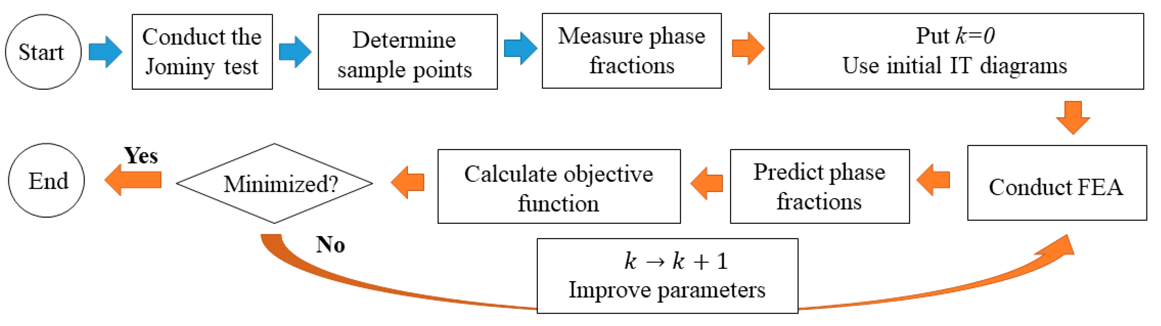
The Jominy end-quench test is one of the most reliable and common methods used to measure the hardenability of steels [13]. It consists of heating a cylindrical steel specimen up to the austenitizing temperature and then rapidly cooling one end to induce the formation of a diverse microstructure composed of different phases including martensite, bainite, ferrite, pearlite and austenite [14,15,16,17]. The Jominy test is likely very appropriate for the calibration of IT or CCT curves obtained from the introduced mathematical models because of the diverse composition of the formed phases in specimen. In this study, the Jominy test is used to improve or optimize the IT diagrams of steels (obtained from Kirkaldy model) by using a finite-element method coupled with an optimization method to minimize the error between experimental Jominy test results and finite-element predictions based on the IT diagrams of the models.

2. Methodology

A finite-element optimization method minimizes the error between the target and predicted phase fractions obtained using the experimental and calculated IT diagrams, respectively. Adjustment parameters applied to the model are the design variables to be determined. Jominy testing of AISI 52100 steel is used to investigate the feasibility and reliability of the method.

Figure 1 presents a conceptual procedure of the methodology for optimizing IT diagrams. First, information about phase fractions at some sample points, called target phase fractions, is obtained on a planar cross-section of the Jominy test sample. The target points are shared with the control points for finite-element predictions and IT diagram optimization. The measured fraction of jth phase at the ith sample point is applied as its associated target value, $X_{j,tar(i)}$, in the following objective function to be minimized [18]:

$${\Psi }_0=\sqrt{\frac{1}{n}{{\displaystyle \sum _{i=1}^n{\displaystyle \sum _{j=1}^m{W}_j\left(X_{j,tar(\mathrm{i})}-X_{j,pre(\mathrm{i})}\right)}}}^2}$$

(1)

where $X_{j,pre(i)}$ and $W_j$ are the fraction of jth phase predicted by the finite element analysis at the ith sample point and a weighting factor for the jth phase, respectively. n and m are the numbers of sample points and phases, respectively. Therefore, the objective function ${\Psi }_0$ is simply defined as the errors at the sample points. The target phase fraction can be determined in an experimental or theoretical way.

To adjust the curves in the IT diagram using some parameters to be optimally determined, two transforming equations are defined as follows:

$$Log(t^{\prime })=aLog(t)+b$$

(2)

$$T^{\prime }=T+c$$

(3)

where $T$ and $t$ are the temperature and time in the untransformed system, respectively, which define the domain in which to express the Kirkaldy model. The parameters $T^{\prime }$ and $t^{\prime }$ are the temperature and time after applying the transforming equations, respectively, and represent the adjusted curves shown in Figure 2. The constants a, b and c are the adjustment parameters, i.e., the so-called design parameters in the optimization problem, which are used to optimally adjust the theoretical IT diagram. Note that adjustment parameters are obtained for each curve in the IT diagram. For example, the parameters for the pearlite start curve are $a_{Ps}$, $b_{Ps}$ and $c_{Ps}$ (Figure 3). Therefore, the total number of design parameters for each phase in the optimization is six, including the adjustment parameters of the start and finish curves.

Koistinen–Marburger’s non-diffusional transformation model [19] is used to calculate the martensite and austenite phase fractions. The martensite starting temperature ($M_s$), obtained using JMatPro software [5], that is almost equal to the experimental value from the reference IT diagram [1]. The optimization problem is thus defined as follows: Determine the design parameters (the constants a, b and c) that minimize the objective function ${\Psi }_0$ subject to some inequality or equality constraints. To optimize the initial IT diagram (the Kirkaldy model), the initial guesses of a, b and c are assumed to be 1.0, 0.0 and 0.0, respectively. During the optimization procedure, the key idea is to identify the adjustment parameters for each phase, i.e., the design parameters, in an iterative way that predicts the phase fractions closest to the target phase fractions in terms of the objective function stated in Equation (1). The global response surface model (GRSM) [20] is used as the optimization technique.

3. Acquisition of the Optimized Parameters

3.1. Thermal Parameters

The Jominy end-quench test of AISI 52100 steel was first analyzed according to the standard ASTM A255 [15] to optimally identify the thermal conditions, which greatly influence the heat transfer analysis. A two-dimensional axisymmetric finite-element model was developed to analyze the heat transfer of the Jominy test using the commercial code AFDEX [21,22,23]. For mesh generation of the simulations, quadrilateral finite-element models were employed.

Table 1. Composition of AISI 52100 steel (wt%).

C	Mn	Si	Ni	Cr	Mo	Fe
1.08	0.53	0.25	0.33	1.46	0.08	Bal.

ASTM Grain size: 7.0.

provides the chemical composition of the steel. In the Jominy test, the specimen is heated to the austenitizing temperature of 850 °C and then cooled at one end by a water spray (Figure 4). The temperature values were recorded at the sample points using type K thermocouple wires with a 1.5-mm diameter and the data acquisition rate was 50.0 Hz [16]. The density of the material was assumed to be constant at 7860 $\mathrm{kg}/{\mathrm{m}}^3$. The heat capacity and thermal conductivity of the steel used in this study were obtained using the JMatPro software [5] at different temperatures and are summarized in

Table 2. Thermal properties of AISI 52100 steel.

T (°C)	900	700	500	300	100
Specific heat $(\mathrm{J}/\mathrm{gK})$	0.60	0.93	0.68	0.56	0.47
Thermal conductivity $(\mathrm{W}/\mathrm{mK})$	27.6	31.4	35.1	37.4	35.2

.

The cylindrical and top surfaces of the specimen, i.e., the free surfaces, are subjected to natural convection and radiation. Heat loss through these free surfaces is analyzed by considering both convection and radiation. The radiation heat transfer from the free surfaces is calculated using the Stefan–Boltzmann law with a radiation emissivity of 0.7 [24]. The convective heat transfer on the surfaces is described by Newton’s law of cooling [24,25]:

$$q_c=Ah(T_s-T_a)$$

(4)

where A, $h$, $T_s$ and $T_a$ are the surface area, convection heat transfer coefficient, surface temperature and ambient temperature, respectively. The parameter h of the free surfaces is calculated using the formulas for natural convection [26]. The convection heat transfer coefficient on the quenched bottom surface, $h_q$, cannot be simply calculated. Notably, $h_q$ has a decisive influence on all the predictions related to the temperature and it is highly dependent on the surface temperature [27]. Thus, optimized convection heat transfer coefficients on the quenched bottom surface are obtained for this study, which are determined by minimizing the difference between the cooling curves obtained from experiments [16] and predictions at specific sample points, i.e., by solving an optimization problem. It is assumed that $h_q$ is temperature dependent and can be linearly interpolated by a set of $h_q$ values at the sampled temperatures, which are optimally determined.

The objective function is as follows:

$${\phi }_0=\sqrt{\frac{1}{n}{\displaystyle \sum _{i=1}^n{\displaystyle \sum _{j=0}^m{(T_{j,\exp (i)}-T_{j,pre(i)})}^2}}}$$

(5)

where $T_{j,pre(i)}$ and $T_{j,\exp (i)}$ are the predicted and experimental temperatures at the ith sample point and jth sampled time during cooling, respectively. The parameters n and m are the number of sample points (1 to 5 in Figure 4) and sampled times, respectively. The experimental temperatures and their corresponding predictions obtained using the optimized $h_q$ values (

Table 3. Optimized convective film coefficients at the quenched end.

T (°C)	20	400	580	650	850
$h_q$$(\mathrm{W}/{\mathrm{m}}^2\mathrm{K}$)	43.8	32.4	31.5	10.6	2.0

) are in good agreement (Figure 5). The maximum difference between the measured and predicted temperatures is about 50 °C at sample points 1 and 2. This error is calculated at temperatures below 300 °C where diffusional phase transformations are not fast enough to influence on the phase fractions.

3.2. Adjustment Parameters of IT Diagram

The Jominy test is simulated using the reference IT diagram of the steel [1] and the optimized thermal conditions obtained in the previous chapter were used to acquire the target phase fraction values for optimization of the adjustment parameters defined in Equations (2) and (3).

Table 4. Coordinates of the sample points and the corresponding predicted phase fractions (vol%).

Sample Point	x (mm)	y (mm)	Austenite	Pearlite	Bainite	Martensite
1	11.4	1.5	5.5	0.0	0.0	94.5
2	11.6	3.1	5.5	0.0	0.0	94.5
3	11.5	5.0	5.5	0.0	0.0	94.5
4	11.6	7.2	5.5	0.0	0.0	94.5
5	11.5	9.0	5.5	0.0	0.0	94.5
6	11.4	11.1	5.5	0.0	0.1	94.4
7	11.3	12.9	5.5	0.0	0.3	94.2
8	11.3	13.4	5.5	0.0	0.4	94.2
9	11.7	15.4	5.5	0.0	0.7	93.8
10	11.7	20.1	5.4	0.3	1.4	92.9
11	11.7	25.3	5.3	1.0	1.8	91.9
12	11.7	30.0	5.3	2.7	1.4	90.7
13	11.3	35.7	5.1	7.3	0.8	86.9
14	11.3	45.2	3.7	33.0	0.1	63.2
15	11.3	50.4	2.1	61.3	0.1	36.5
16	11.3	55.1	0.6	89.2	0.0	10.2
17	11.3	60.3	0.0	99.5	0.0	0.4
Average	-	-	4.5	17.3	0.41	77.7

lists the target values calculated at the 17 sample points on the planar cross-sectio of the specimen shown in Figure 6.

The optimization of the IT curves, i.e., the optimal calculation of the adjustment parameters defined in Equations (2) and (3), is realized by iteratively reducing the error of the phase fraction between experiments and predictions at the 17 sample points using the HyperSTUDY optimization tool [28,29]. The global response surface method (GRSM) [20] which is a response surface-based approach is employed. In this method, the response surface-based optimization makes a few designs at each iteration. Extra designs are also created globally to find the other probable responses. All the designs in an iteration are solved in parallel to reduce the optimization time. To ensure a better adaptation of the model, the response surface is updated adaptively with the newly generated designs [28].

For AISI 52100 steel, four curves in the IT diagram including pearlite and bainite start and finish (Figure 2) should be optimally adjusted. The optimization variables are thus $a_{Ps}$, $b_{Ps}$ and $c_{Ps}$ for pearlite start, $a_{Pf}$, $b_{Pf}$ and $c_{Pf}$ for pearlite finish, $a_{Bs}$, $b_{Bs}$ and $c_{Bs}$ for bainite start and $a_{Bf}$, $b_{Bf}$ and $c_{Bf}$ for bainite finish. The constraints on the adjustment parameters are assigned as follows:

$$0.1\le a\le 5.0$$

(6)

$$-5.0\le b\le 5.0$$

(7)

$$-30.0\le c\le 30.0$$

(8)

where a includes $a_{Ps}$, $a_{Pf}$, $a_{Bs}$ and $a_{Bf}$; b includes $b_{Ps}$, $b_{Pf}$, $b_{Bs}$ and $b_{Bf}$; and c includes $c_{Ps}$, $c_{Pf}$, $c_{Bs}$ and $c_{Bf}$. The initial guesses used are $a_0=1.0,b_0=0.0$ and $c_0=0.0$ for every phase. These initial guesses provide the same IT diagram with the modified Kirkaldy model for the medium and high alloy steels [5] and the diagram approaches the experimental one through optimization, i.e., minimization of the objective function defined in Equation (1). Two optimizations using different weighting factors, $W_j$ values, were performed as shown in

Table 5. Weighting factors in the optimization cases.

Optimization Cases	${\mathit{W}}_{\mathit{A}\mathit{u}\mathit{s}\mathit{t}\mathit{e}\mathit{n}\mathit{i}\mathit{t}\mathit{e}}$	${\mathit{W}}_{\mathit{P}\mathit{e}\mathit{a}\mathit{r}\mathit{l}\mathit{i}\mathit{t}\mathit{e}}$	${\mathit{W}}_{\mathit{B}\mathit{a}\mathit{i}\mathit{n}\mathit{i}\mathit{t}\mathit{e}}$	${\mathit{W}}_{\mathit{M}\mathit{a}\mathit{r}\mathit{t}\mathit{e}\mathit{n}\mathit{s}\mathit{i}\mathit{t}\mathit{e}}$
Case 1	0.25	0.25	0.25	0.25
Case 2	0.089	0.017	0.885	0.009

. In Case 1, the same weighting factors were applied to all phases of Equation (1). In Case 2, the weighting factors were allocated unequally in terms of the average phase fractions shown in Table 4; more significance was assigned to phases present in smaller fractions, such as bainite and austenite. In both cases, optimizations were carried out independently for pearlite and bainite. As shown in Figure 7, after about 350 iterations, the objective function values of Cases 1 and 2 converged to 0.039 and 0.001, respectively.

Table 6. Optimized adjustment parameters.

Optimization Cases.	Pearlite Start			Pearlite Finish			Bainite Start			Bainite Finish
	$a_{Ps}$	$b_{Ps}$	$c_{Ps}$	$a_{Pf}$	$b_{Pf}$	$c_{Pf}$	$a_{Bs}$	$b_{Bs}$	$c_{Bs}$	$a_{Bf}$	$b_{Bf}$	$c_{Bf}$
Case 1	2.10	−2.84	3.1	2.58	−4.80	3.7	0.14	1.21	−5.1	0.81	0.48	−8.3
Case 2	2.08	−2.85	−1.3	2.58	−4.78	2.6	0.71	0.05	25.1	0.95	−0.17	−6.3

lists the optimized adjustment parameters for both cases. Figure 7 shows that for Case 1, the reduction of the objective function values for the bainite curves is quite small compared with those of the pearlite, indicating that optimization cannot adjust the bainite curves appropriately. In contrast, the value of the objective function is reduced during both the pearlite and bainite optimizations of Case 2, where weighting factors are applied.

To investigate the effect of number of elements on the optimized adjustment parameters, optimizations of pearlite curves (Case 2) were conducted with four finite element models of 500, 1000, 2000 and 4000 elements. The effect of the number of elements on the normalized adjustment parameters for pearlite curves with respect to the 4000-element model is shown in Figure 8. As depicted, by increasing the number of elements, the results become more reliable and the dispersion of optimized values decreases. However, the optimized values are less scattered when the number of elements is greater than 2000. The larger the number of elements, the longer is the optimization time. Therefore, a sufficient number of elements that is 2000 used not only to save the time but also to achieve a reliable result.

4. Results and Discussion

4.1. Validation

Figure 9 presents the IT diagrams obtained using experiments, the Kirkaldy model and the optimized models (Cases 1 and 2). There is a considerable difference between the experimental IT diagram and the initial IT diagram obtained from the Kirkaldy model. Applying the optimized adjustment parameters obtained from both optimizations enhances the Kirkaldy model and reduces the gap between the experiments and model significantly. Both of the start and finish curves of the pearlite phase transformation are in good agreement with the associated curves in the experimental IT diagram when the optimized adjustment parameters obtained from Cases 1 and 2 are applied. The difference between the experiments and model for the bainite curves is also reduced in both cases. However, considerable differences are evident between the experimental start and finish curves of bainite and those of Case 1. This is due to the small fractions of bainite at the sample points compared with the other phases, particularly martensite. The average bainite fraction at the sample points is 0.41 vol%, which is smaller than the average fraction of any other phase (Table 4). Thus, the objective function during optimization is greatly affected by the pearlite start and finish curves, resulting in a more efficient optimization for the pearlite curves. As is evident in Figure 9, the optimized model of Case 2 yields acceptable curves for both the bainite and pearlite transformations because weighting factors are applied to the objective function.

Figure 10 illustrates the distribution of austenite, pearlite, bainite, and martensite fractions predicted using the experimental IT diagrams, Kirkaldy model, and optimized IT diagrams using both optimizations. The same finite-element model given in Section 3 was applied for all simulations, and only the IT diagrams used in the simulations are different. Figure 10 clearly shows qualitative improvements in predictions with the optimized adjustment parameters. The distribution of the predicted phase fractions of all phases is similar to that predicted using the experimental IT diagrams. However, the maximum predicted bainite fractions are 2.0 vol%, 1.1 vol% and 1.8 vol% (Figure 10c) in the experimental IT diagrams and optimization Cases 1 and 2, respectively. The distribution of the bainite fraction in Case 2 is in adequate agreement with the predicted distribution using experimental IT diagrams. Note that the predictions of the Kirkaldy model are in very poor agreement with the predictions of the experimental IT diagrams.

Figure 11 quantitatively compares the phase fractions predicted using the experimental IT diagrams with those of the original and optimized Kirkaldy models. The R-squared values of the austenite, pearlite and martensite phases predicted by Case 1 of the optimized Kirkaldy model are 0.94, 0.97 and 0.92, respectively, indicating that the error between the experimental data and the optimized Kirkaldy model (Case 1) is negligible. The R-squared value for the bainite phase is 0.41, which is very far from 1.0. However, the data points for the bainite fractions predicted by the Case 1 are less scattered in Figure 11c compared with the Kirkaldy model. By applying the optimized Kirkaldy model of Case 2, the R-squared values for austenite, pearlite, bainite and martensite improve to 0.94, 0.97, 0.96 and 0.92, respectively.

To thoroughly evaluate the optimized models, the phase fractions are predicted at 40 sample points distributed uniformly on the plane section of the Jominy test specimen. Note that these sample points are not identical to the sample points used in the optimization for training the model (Table 4). Therefore, they can be used to evaluate the reliability of the model. Figure 12 shows that the average R-squared values are 0.9982 and 0.9994 for Cases 1 and 2, respectively. Both are very close to 1.0, demonstrating that the optimized models can predict the phase fractions of all phases with high confidence. However, the IT diagrams of Case 2 lie closer to the experimental IT diagrams than do those of Case 1, indicating that the optimized model of Case 2 better predicts the fractions of all phases, even those of phases with small fractions (such as bainite). In other words, optimization using an objective function balanced with weighting factors reliably predicts the phase fractions not only of the Jominy test (where the bainite and austenite fractions are small), but also of other heat treatment processes.

4.2. Practical Case Study

We used the above method to adjust the IT diagrams of 100CrMnSi6 (the chemical composition is given in

Table 7. Composition of 100CrMnSi6 steel (wt%).

C	Mn	Si	P	Cr	Al	Ti	Fe
0.99	1.1	0.62	0.11	1.52	0.26	0.2	Bal.

). The Jominy test was performed using the ASTM A255 standard. The fractions of pearlite at the sample points of Figure 13 were measured via optical metallography (OM). For metallographic observation, the samples were polished and etched with 1% (v/v) nital. The OM images at certain sample points are depicted in Figure 14 and the measured perlite fractions given in

Table 8. Coordinates of the sample points and the corresponding measured phase fractions (vol%).

Sample Point	x (mm)	y (mm)	Pearlite	Bainite	Martensite + Retained Austenite
1	7.5	9.0	1.0	2.0	97.0
2	7.5	11.0	7.0	6.0	87.0
3	7.5	13.0	14.0	4.0	82.0
4	7.5	15.0	29.0	2.0	69.0
5	7.5	30.0	95.0	0.0	5.0
Average			29.2	2.8	68.0
Weighting factor			0.085	0.879	0.036

. The fraction of pearlite with black is measured by the imageJ software. As it is shown in Figure 14, at the sample point 2, 3 and 4, the microstructure contains 7.0, 14.0 vol% and 29.0 vol% of pearlite, respectively. The rest of the microstructure is composed of the bainite and martensite. From sample points 1 to 5, increasingly distant from the quenched end of the Jominy sample, the pearlite fraction increased from 1.0 vol% to 95.0 vol%.

The bainite and martensite fractions were measured via scanning electron microscopy (SEM) and image analysis. Figure 15 shows the SEM images of some sample points; the calculated bainite and martensite fractions are listed in Table 8. The microstructure features pearlite, bainite and martensite at sample points 3 and 4 but is almost entirely pearlite at sample point 5.

After measuring the fractions of pearlite, bainite and martensite at certain sample points, a finite-element optimization method with weighting factors (Case 2) was employed to adjust the initial IT diagrams. The weighting factors were allocated in terms of the average phase fractions shown in Table 8. The weighting factor multiplied by the average of phase fraction is constant for all phases. The initial diagrams (Figure 16) were obtained using the modified Kirkaldy model for the medium and high alloy steels after inputting chemical compositions and grain sizes [5]. The thermal properties of 100CrMnSi6 [5] and the optimized thermal conditions described in Chapter 3, were input to the finite-element model. The A_cm, A₁ and martensite start, and finish temperatures were 883, 768, 100 and 17 °C, respectively.

The adjustment parameters yielded by minimizing the error between the predicted and measured phase fractions at the given sample points are listed in

Table 9. Optimized adjustment parameters.

Pearlite Start			Pearlite Finish			Bainite Start			Bainite Finish
$a_{Ps}$	$b_{Ps}$	$c_{Ps}$	$a_{Pf}$	$b_{Pf}$	$c_{Pf}$	$a_{Bs}$	$b_{Bs}$	$c_{Bs}$	$a_{Bf}$	$b_{Bf}$	$c_{Bf}$
0.96	−0.99	13.83	1.09	−0.73	−9.57	0.90	−1.49	4.51	1.00	−1.39	2.64

. Adjusted IT diagrams are depicted in Figure 16; these clearly differ from the initial diagrams. In Figure 17, the phase fractions predicted by the adjusted IT diagrams are compared to those measured at the sample points; the predicted and measured phase fractions are in excellent agreement when the adjustment parameters are applied.

5. Conclusions

Herein, a new method for adjusting an isothermal transformation diagram is described. The method uses the finite-element solution, practical experiments including the measured phase fractions at designated sample points and optimization techniques. Adjustment parameters defined on the Kirkaldy model are used as design variables in the optimization, which minimizes the objective error function between the target and predicted phase fractions at the sample points. In this way, three adjustment parameters for each curve in isothermal transformation diagram can be obtained. The results are summarized as follows:

The method is practical and feasible because it can adjust the Kirkaldy model for general steels using a standard Jominy test.

The results show that the Kirkaldy model can reliably predict phase fractions after applying the optimized adjustment parameters. The isothermal transformation diagrams obtained from the Kirkaldy model provide the initial guesses for the optimization.

Optimizing the adjustment parameters enables the initial guesses to approach the experimental isothermal transformation diagram.

The error between the predicted phase fractions using the adjusted model and the experimental isothermal transformation diagrams is sufficiently small for practical use. The practicability of the method is shown by adjusting the isothermal transformation diagrams for 100CrMnSi6 bearing steel.

References

1. Vander Voort, G.F. Atlas of Time-Temperature Diagrams; ASM International: Novelty, OH, USA, 1991. [Google Scholar]
2. Kirkaldy, J.S. Prediction of microstructure and hardenability in low alloy steels. In Proceedings of the International Conference on Phase Transformation in Ferrous Alloys, Philadelphia, PA, USA, 4–6 October 1983. [Google Scholar]
3. Li, M.V.; Niebuhr, D.V.; Meekisho, L.L.; Atteridge, D.G. A computational model for the prediction of steel hardenability. Metal. Mater. Trans. B 1998, 29, 661–672. [Google Scholar] [CrossRef]
4. Åkerström, P.; Oldenburg, M. Austenite decomposition during press hardening of a boron steel—Computer simulation and test. J. Mater. Process. Technol. 2006, 174, 399–406. [Google Scholar] [CrossRef]
5. Saunders, N.; Guo, U.K.Z.; Li, X.; Miodownik, A.P.; Schillé, J.P. Using JMatPro to model materials properties and behavior. JOM 2003, 55, 60–65. [Google Scholar] [CrossRef]
6. Johnson, W.; Mehl, R. Reaction kinetics in processes of nucleation and growth. Trans. Am. Inst. Min. Metall. Eng. 1939, 135, 416–458. [Google Scholar]
7. Avrami, M. Kinetics of phase change I. J. Chem. Phys. 1939, 7, 1103–1112. [Google Scholar] [CrossRef]
8. Kolmogorov, A. K statistiches koi teorii kristallizatsii metallov. Izv. Akad. Nauk USSR Ser. Matemat. 1937, 3, 355–359. [Google Scholar]
9. Bok, H.H.; Lee, M.G.; Pavlina, E.J.; Barlat, F.; Kim, H.D. Comparative study of the prediction of microstructure and mechanical properties for a hot-stamped B-pillar reinforcing part. Int. J. Mech. Sci. 2011, 53, 744–752. [Google Scholar] [CrossRef]
10. Cahn, J.W. Transformation kinetics during continuous cooling. Acta Metall. 1956, 4, 572–575. [Google Scholar] [CrossRef]
11. Szeliga, D.; Gawad, J.; Pietrzyk, M. Inverse analysis for identification of rheological and friction models in metal forming. Comput. Methods Appl. Mech. Eng. 2006, 195, 6778–6798. [Google Scholar]
12. De Bono, D.M.; London, T.; Baker, M.; Whiting, M.J. A robust inverse analysis method to estimate the local tensile properties of heterogeneous materials from nano-indentation data. Int. J. Mech. Sci. 2017, 123, 162–176. [Google Scholar] [CrossRef] [Green Version]
13. Pietrzyk, M.; Kusiak, J.; Kuziak, R.; Madej, Ł.; Szeliga, D.; Gołąb, R. Conventional and multiscale modeling of microstructure evolution during laminar cooling of DP steel strips. Metall. Mater. Trans. A 2014, 45, 5835–5851. [Google Scholar] [CrossRef] [Green Version]
14. ASTM A255-10(2018), Standard Test Methods for Determining Hardenability of Steel; ASTM International: West Conshohocken, PA, USA, 2018; Available online:www.astm.org.
15. Çakir, M.; Özsoy, A. Investigation of the correlation between thermal properties and hardenability of Jominy bars quenched with air–water mixture for AISI 1050 steel. Mater. Des. 2011, 32, 3099–3105. [Google Scholar] [CrossRef]
16. Lee, S.-J.; Pavlina, E.J.; van Tyne, C.J. Kinetics modeling of austenite decomposition for an end-quenched 1045 steel. Mater. Sci. Eng. A 2010, 527, 3186–3194. [Google Scholar] [CrossRef]
17. Fong, H.S. Further observations on the Jominy end quench test. J. Mater. Process. Technol. 1993, 38, 221–225. [Google Scholar] [CrossRef]
18. Irani, M.; Lim, S.; Joun, M. Experimental and numerical study on the temperature sensitivity of the dynamic recrystallization activation energy and strain rate exponent in the JMAK model. J. Mater. Res. Technol. 2018. [Google Scholar] [CrossRef]
19. Koistinen, D.P.; Marburger, R.E. A general equation prescribing the extent of the austenite-martensite transformation in pure iron-carbon alloys and plain carbon steels. Acta Metall. 1959, 7, 59–60. [Google Scholar] [CrossRef]
20. Kleijnen, J.P.C. Response surface methodology for constrained simulation optimization: An overview. Simul. Model. Pract Theory 2008, 16, 50–64. [Google Scholar] [CrossRef]
21. Eom, J.G.; Son, Y.H.; Jeong, S.W.; Ahn, S.T.; Jang, S.M.; Yoon, D.J.; Joun, M.S. Effect of strain hardening capability on plastic deformation behaviors of material during metal forming. Mater. Des. (1980–2015) 2014, 54, 1010–1018. [Google Scholar] [CrossRef]
22. Joun, M.; Eom, J.G.; Lee, M.C. A new method for acquiring true stress–strain curves over a large range of strains using a tensile test and finite element method. Mech. Mater. 2008, 40, 586–593. [Google Scholar] [CrossRef]
23. Lee, M.C.; Chung, S.H.; Jang, S.M.; Joun, M.S. Three-dimensional simulation of forging using tetrahedral and hexahedral elements. Finite Elem. Anal. Des. 2009, 45, 745–754. [Google Scholar] [CrossRef]
24. Bergman, T.L.; Lavine, A.S.; Incropera, F.P.; DeWitt, D.P. Fundamentals of Heat and Mass Transfer, 8th ed.; Binder Ready Version; John Wiley and Sons Ltd.: Chichester, UK, 2011. [Google Scholar]
25. Chapman, A.J.; Chapman, A.J. Fundamentals of Heat Transfer; Macmillan: New York, NY, USA; Collier Macmillan: London, UK, 1987. [Google Scholar]
26. Bamberger, M.; Prinz, B. Determination of heat transfer coefficients during water cooling of metals. Mater. Sci. Technol. 1986, 2, 410–415. [Google Scholar] [CrossRef]
27. Nunura, C.R.N.; dos Santos, C.A.; Spim, J.A. Numerical–Experimental correlation of microstructures, cooling rates and mechanical properties of AISI 1045 steel during the Jominy end-quench test. Mater. Des. 2015, 76, 230–243. [Google Scholar] [CrossRef]
28. HyperStudy User Manual; Altair Engineering Inc.: Troy, MI, USA, 2009.
29. Irani, M.; Joun, M. Determination of JMAK dynamic recrystallization parameters through FEM optimization techniques. Comput. Mater. Sci. 2018, 142, 178–184. [Google Scholar] [CrossRef]
Figure 1. Conceptual procedure of the presented method for adjusting isothermal transformation diagrams.
Metals 10 00931 g001
Figure 2. Transformation from the Tt system to the T t system.
Metals 10 00931 g002
Figure 3. Experimental isothermal transformation diagrams and Kirkaldy model of AISI 52100 steel.
Metals 10 00931 g003
Figure 4. Sample points for the temperature measurements (dimensions in mm).
Metals 10 00931 g004
Figure 5. Measured and predicted cooling curves at the sample points.
Metals 10 00931 g005
Figure 6. Finite-element model and the sample points.
Metals 10 00931 g006
Figure 7. Variation of the objective function as a function of iteration number.
Metals 10 00931 g007
Figure 8. Variation in the normalized adjustment parameters according to the number of elements.
Metals 10 00931 g008
Figure 9. Optimized Kirkaldy model with experimental isothermal transformation diagrams and the Kirkaldy model.
Metals 10 00931 g009
Figure 10. Comparison of the phase fractions (vol%) predicted by the three models. (a) Austenite; (b) pearlite; (c) bainite and (d) martensite.
Metals 10 00931 g010
Figure 11. Predicted phase fractions using the original and adjusted Kirkaldy models. (a) Austenite, (b) pearlite; (c) bainite; and (d) martensite.
Metals 10 00931 g011
Figure 12. Predicted phase fractions using the experimental and adjusted Kirkaldy models.
Metals 10 00931 g012
Figure 13. Sample points for phase fraction measurements.
Metals 10 00931 g013
Figure 14. Optical metallography images at (a) sample points 2; (b) sample points 3 and (c) sample points 4 (dark phase is pearlite and the light phases are martensite, bainite or retained austenite).
Metals 10 00931 g014
Figure 15. SEM images of sample points at (a) sample point 3; (b) sample point 4 and (c) sample point 5. (phases are labeled in the images).
Metals 10 00931 g015
Figure 16. Adjusted Kirkaldy model with Jominy test and the initial Kirkaldy model.
Metals 10 00931 g016
Figure 17. Predicted and measured phase fractions at certain sample points.
Metals 10 00931 g017