Atmospheric Corrosion Sensor Based on Strain Measurement with Active–Dummy Fiber Bragg Grating Sensors

Abstract

Using the relationship between strain and thickness from the materials theory, this paper presents further development of the atmospheric corrosion sensor based on strain measurement (ACSSM). Fiber Bragg grating (FBG) sensors were used to measure strain in this study. The active–dummy method was employed to compensate the effects of environmental temperature drift, with the configuration and position of the active–dummy FBG sensors determined based on simulations conducted using the finite element method (FEM). Hence, the reduction in thickness of low-carbon steel test pieces could be isolated, ensuring accurate characterization of this parameter. Results of practical galvanostatic electrolysis experiments conducted with the FBG sensors in the proposed configuration demonstrated accurate measurement of the reduction in the thickness of a test piece, suggesting that an ACSSM with active–dummy FBG sensors would be appropriate for monitoring of atmospheric corrosion in steel structures.

1. Introduction

Since corrosion is the main failure mode for steel structures, sensors that can predict their corrosion rate are very important in structural health monitoring for evaluating safety levels [1]. The detection of losses in weight and thickness [2,3] and electrochemical impedance spectroscopy [4,5] are techniques that have been proposed for atmospheric corrosion monitoring. Although the former methods are capable of measurement to a high degree of accuracy, they do not provide real time monitoring, and the cost of chemicals required for removing the corrosion product is high. Similarly, while electrochemical methods allow in situ corrosion monitoring, a precise measurement is difficult as the sensitivity of these techniques to corrosion reactions affects their operation. Thus, a highly accurate in situ sensor capable of monitoring atmospheric corrosion is needed. Based on this requirement, we developed the atmospheric corrosion sensor based on strain measurement (ACSSM).

In previous ACSSM studies [6,7,8], the reduction of the thickness of a test piece due to corrosion was evaluated using elastic strain by applying a bending moment to the test piece. The mechanical principles of the changes to elastic strain due to reductions in thickness produced by corrosion were devised from theoretical formulas and studies of finite element method (FEM) simulations, using galvanostatic electrolysis as a model for corrosion. Although the actual strain to be measured for evaluation of the reduction of thickness is very small, for long monitoring periods, the strain gauge is subject to large amounts of noise due to changes in the environmental temperature. Hence, we fabricated an original strain measurement circuit with active–dummy circuits for the ACSSM [7,8], which obtained results in good agreement with the mechanical principles devised. However, changes in strain due to a reduction in thickness were very small, and there was a 12% difference between the thicknesses estimated using strain and those obtained by measuring the actual dimensions and the weight loss of the test piece.

In the last decade, many optical fiber techniques have been used such as distributed fiber sensors [9,10], low coherent optical fiber interferometer [11,12], and long period grating sensors [13,14] for strain measurements including fiber Bragg grating (FBG) sensors that were used in this research. FBG has been used in many structural healthy monitoring applications, such as monitoring strain in a metal bridge [15], strain in a concrete structure [16], the stretching of cables in a gymnasium structure [17], the displacement of a landslide [18], detecting the welding joints in a structure [19], and monitoring strain in material for aircraft [20]. Several FBG-based methods, such as FBG sensors embedded in metal film coatings [21,22] and sensors with etched metal cladding for increased sensitivity [23,24], have been proposed for corrosion monitoring in steel structures. Moreover, such sensors have exhibited good sensitivity to the progression of corrosion, even when embedded in concrete [25,26,27]. Since strain measurements using FBG sensors are accurate, of high resolution, and stable, we have modified our ACSSM technique to include active–dummy FBG sensors. In the study, to accurately evaluate the reduction in the thickness of the test piece, the configuration and install positions of the active and dummy FBG sensors were determined through FEM analysis of the effect of temperature on the strain measurement. In addition, we verified the accuracy of the active–dummy FGB sensors’ estimation of reductions in thickness due to corrosion using laboratory experiments based on galvanostatic electrolysis [28].

The operating principle of the ACSSM technique is the measurement of the reduction in thickness of a test piece using the mechanical theory of deformation. An illustration of how this theory is applied is shown in Figure 1. Here, a test piece with a thickness h is deformed elastically according to the radius of curvature, ρ, and the center angle, dθ. The neutral plane (N-N) is unaltered by the deformation. The shortened curvature in the compressed strain position (C-C) where the FBG sensor is installed is equal to $\left(\rho -\frac{h}{2}\right)\mathrm{d}\theta$. The strain on the compressed surface can be expressed by [6,7]:

$$\epsilon =\frac{\left(\rho -\frac{h}{2}\right)\mathrm{d}\theta -\rho \mathrm{d}\theta }{\rho \mathrm{d}\theta }=-\frac{h}{2\rho }$$

(1)

If the thickness of the test piece is decreased due to corrosion, the distance between the neutral plane and the surface under the corroded area is decreased, as shown in Figure 1b. From (1), assuming that ρ >> h, the change in strain can be expressed as

$$\Delta h=2\rho ·\Delta \epsilon$$

(2)

Hence, according to the above, for a constant value of ρ, the change in the strain of the concave surface determines the change in the thickness of the test piece. To ensure that the test piece is subject only to elastic deformation, the minimum value of ρ is calculated as follows [6]:

$$\rho =\frac{Eh}{2\sigma }$$

(3)

where σ is the yield stress of the test piece, and E is its Young’s modulus.

The operation of the FBG strain sensor is based on the measurement of the shift in the Bragg wavelength, which is caused by changes in strain, temperature, and other external influences. In unstrained conditions, the Bragg wavelength (λ_B) is given by [23,25]:

λ_B = 2·n·Λ

(4)

where n is the refractive index and Λ is the spacing between the gratings. When there is a force and temperature from the external environment, both the refractive index and the spacing between the gratings change, and the Bragg wavelength is shifted accordingly:

λ_B = 2·n·ΔΛ + 2Δn·Λ

(5)

where ΔΛ is the change in spacing between gratings and Δn is the change in the refractive index. The changes in the Bragg wavelength due to temperature and strain can be determined by using (5), where the first and second term represent the changes due to strain and temperature, respectively, in [29]:

$$\Delta {\lambda }_B=\left[k\epsilon +\left({\alpha }_{\Lambda }+{\alpha }_n\right)\Delta T\right]{\lambda }_B$$

(6)

where k is a gauge factor, α_Λ is the thermal expansion coefficient, α_n is the thermo-optic coefficient, and ΔT is the change in temperature.

2. Materials and Methods

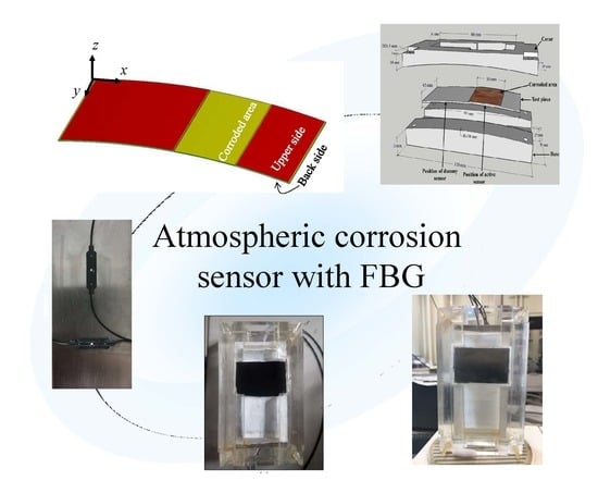
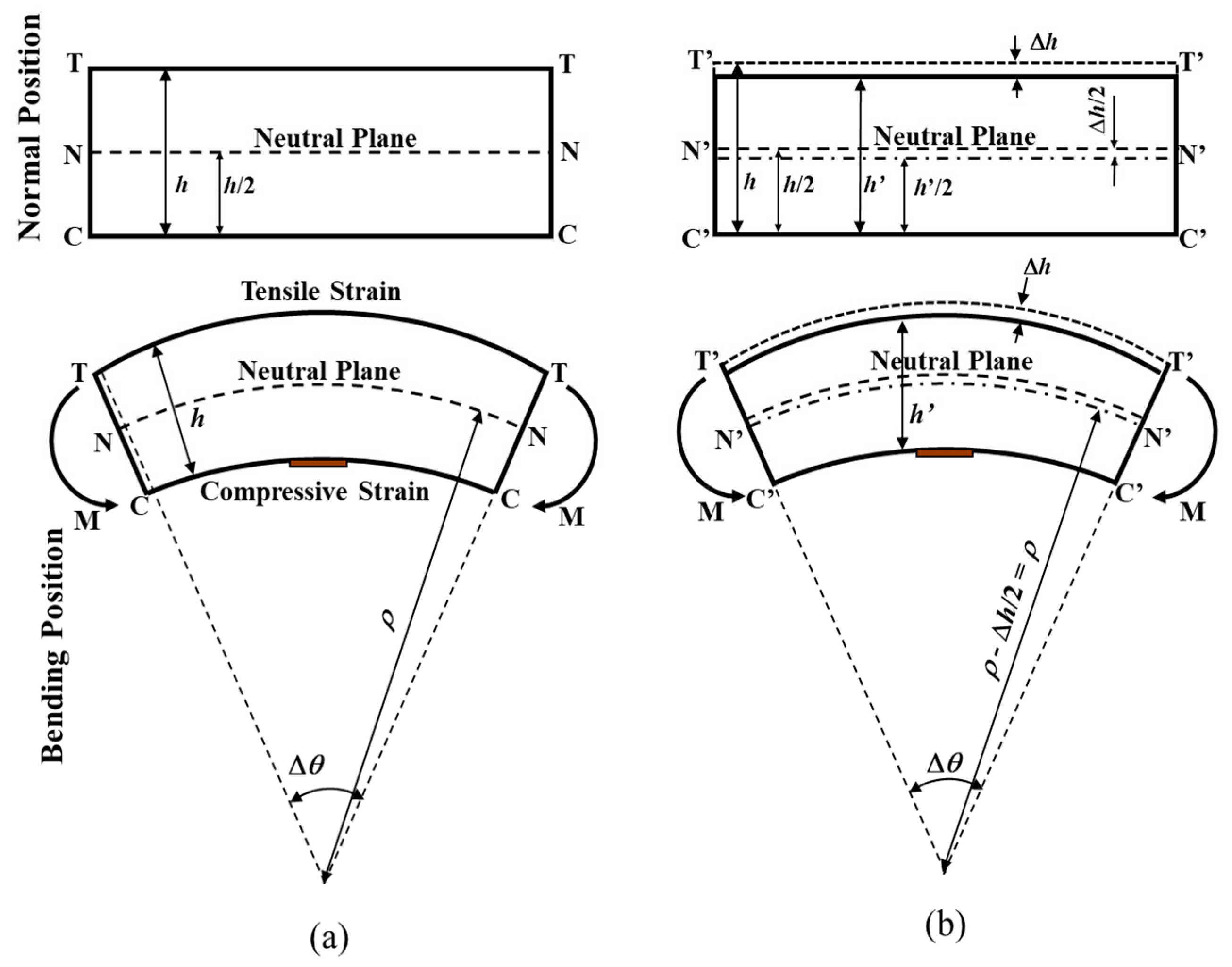
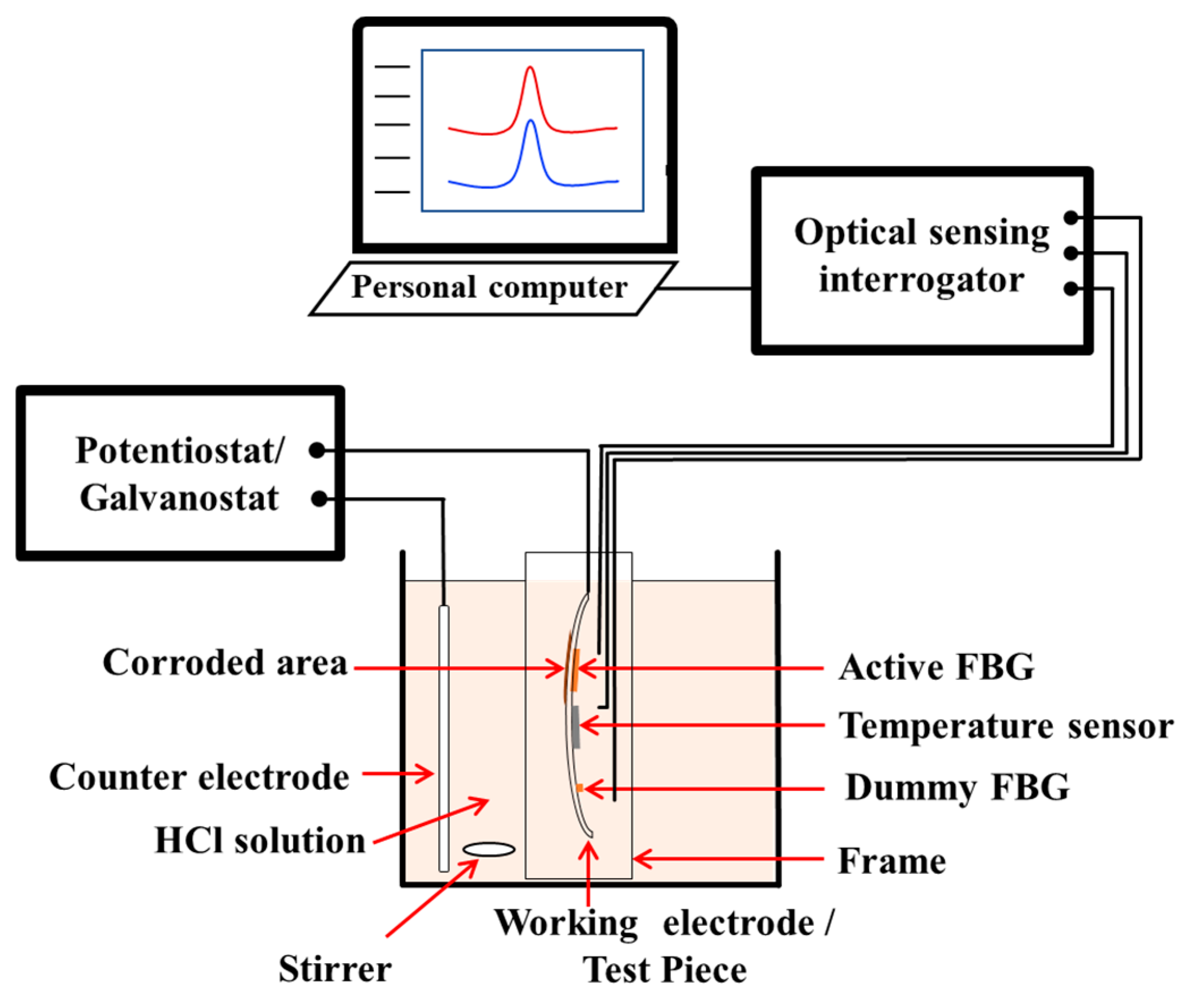
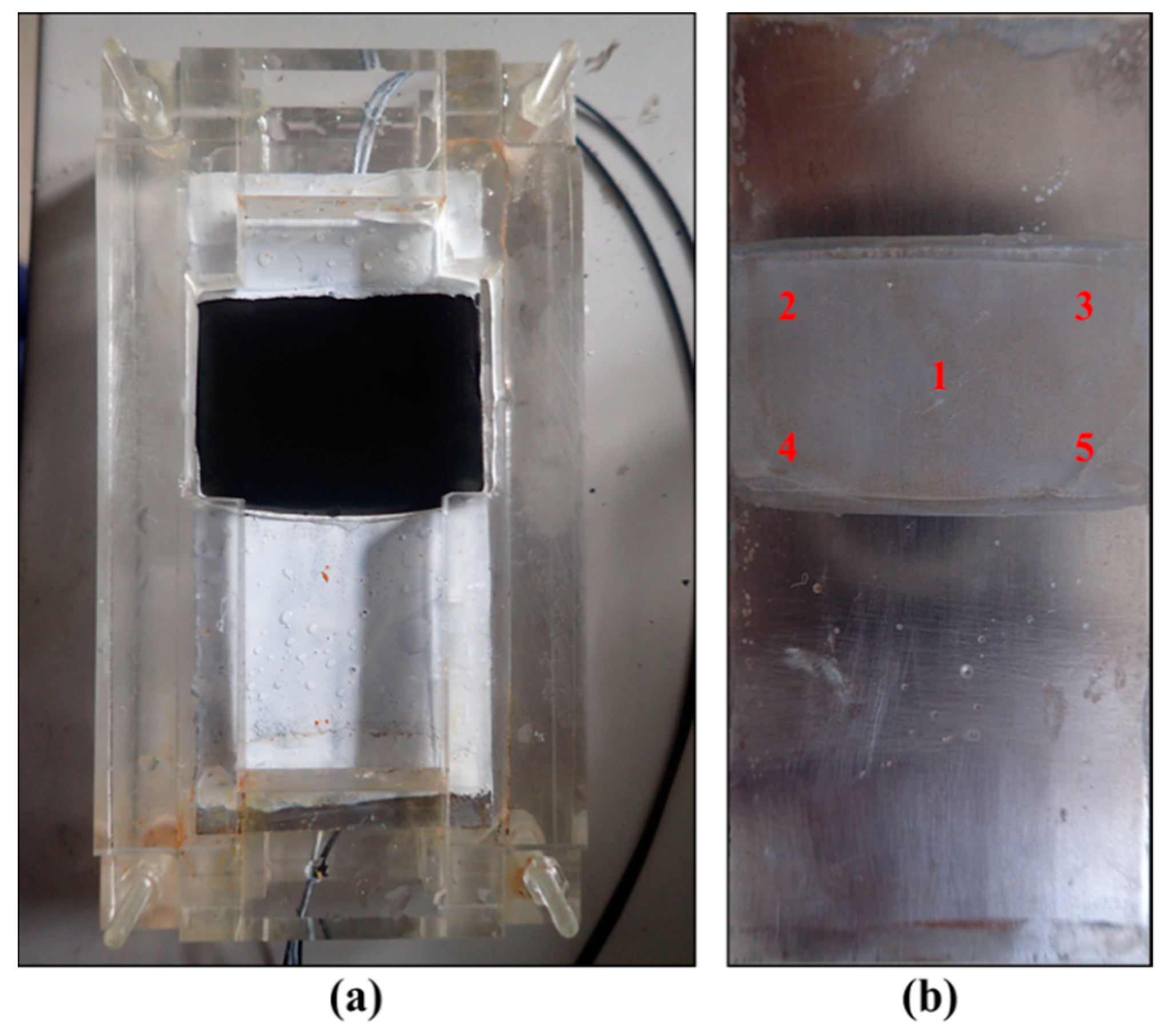
2.1. Experimental Apparatus

Figure 2 shows a diagram of the experimental apparatus, which comprises a base and cover made of polyvinyl chloride. The test piece was 95 mm in length, 45 mm in width, and 0.5 mm in thickness. A 1350 mm² area (30 mm × 45 mm) of the test piece was exposed to facilitate the corrosion representative of the reaction occurring in the rest of the steel structure. The reduction in the thickness of this corroded area enabled verification of the detection principle. The FBGs were installed in the back side of the test piece in the apparatus. The low-carbon material used for the test piece has a Young’s modulus of 210 GPa and a yield stress of 240 MPa. Hence, the minimum value of ρ can be determined to be ~218.75 mm, using (3). To prevent local plastic deformation, the value of ρ was designed to be 430 mm, ~2 times as large as the minimum.

2.2. Measurement Using the Active–Dummy Method

The active–dummy method employed with the ACSSM requires the use of two FBG sensors (an active sensor and a dummy sensor) with different functions. ε_A and ε_D, respectively, the outputs of the active and dummy FBG sensors in με can be expressed as follows:

$${\epsilon }_{\mathrm{A}}=\left(\frac{\Delta {\lambda }_{\mathrm{BA}}}{k{\lambda }_{\mathrm{BA}}}\right)-\frac{1}{k}\left({\alpha }_{\mathsf{\Lambda }}+{\alpha }_{\mathrm{n}}\right)\Delta \mathrm{T}$$

(7)

$${\epsilon }_{\mathrm{D}}=\left(\frac{\Delta {\lambda }_{\mathrm{BD}}}{k{\lambda }_{\mathrm{BD}}}\right)-\frac{1}{k}\left({\alpha }_{\mathsf{\Lambda }}+{\alpha }_{\mathrm{n}}\right)\Delta \mathrm{T}$$

(8)

where λ_BA and λ_BD are the initial wavelengths, and Δλ_BA and Δλ_BD are changes in the wavelength of the active and dummy FBG sensors, respectively, in nm. Therefore, Δε_AD, the difference between the strain in both sensors in με, is expressed as follows:

$$\Delta {\epsilon }_{\mathrm{AD}}={\epsilon }_{\mathrm{A}}-{\epsilon }_{\mathrm{D}}=\left(\frac{\Delta {\lambda }_{\mathrm{BA}}}{k{\lambda }_{\mathrm{BA}}}\right)-\left(\frac{\Delta {\lambda }_{\mathrm{BD}}}{k{\lambda }_{\mathrm{BD}}}\right)$$

(9)

Inspection of (9) highlights that with the active–dummy method, the dependence of the output of both sensors on ΔT has been removed. Hence, unlike the systems described in [30,31,32,33], no additional temperature sensor is required to calculate strain. Moreover, with appropriate configuration, ε_A characterizes both the strain due to the reduction in the test piece’s thickness and strain due to environmental factors, while ε_D characterizes only the strain due to environmental factors. Hence, using Δε_AD, the strain from reductions in thickness due to corrosion can be isolated, enabling more accurate measurement.

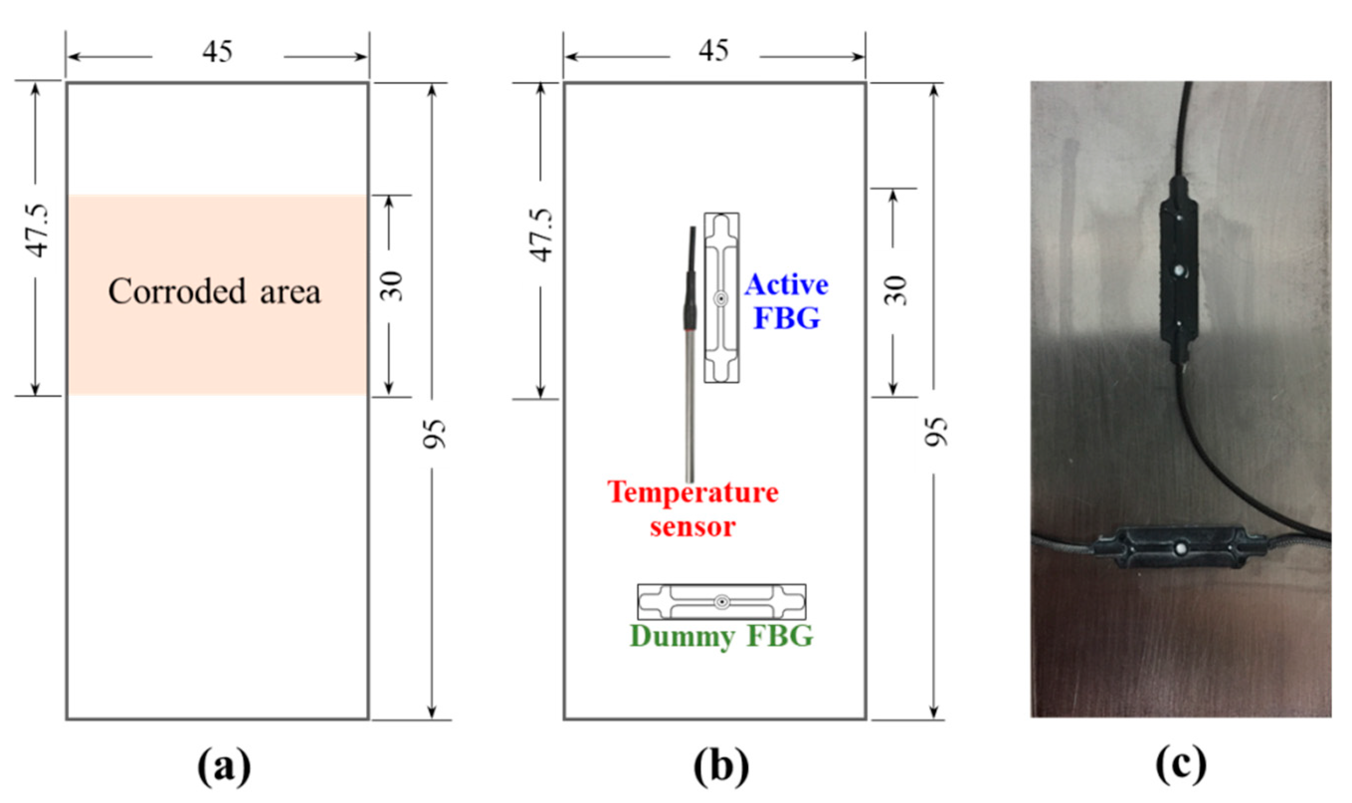
2.3. Configuration of FBG Sensors on the Test Piece

Two os3200 FBG sensors from Micron Optic with initial wavelengths of 1548 nm and k = 0.796 were used as active and dummy sensors in experiments to monitor the strain on the test piece. To verify the operation of the active–dummy method, an additional os4200 FBG sensor from Micron Optic with an initial wavelength λ of 1556 nm was used as a temperature sensor.

Figure 3 shows the configuration of the FBG sensors on the test piece. Sensors were placed on the reverse of the corroded area of the test piece (Figure 3a) in the configuration shown in Figure 3b. The active FBG sensor was placed parallel to the longitudinal axis, while the dummy FBG sensor was placed parallel to the transverse direction of the test piece in the compressed curve apparatus. An actual figure of the FBG sensors in the test piece is shown in Figure 3c.

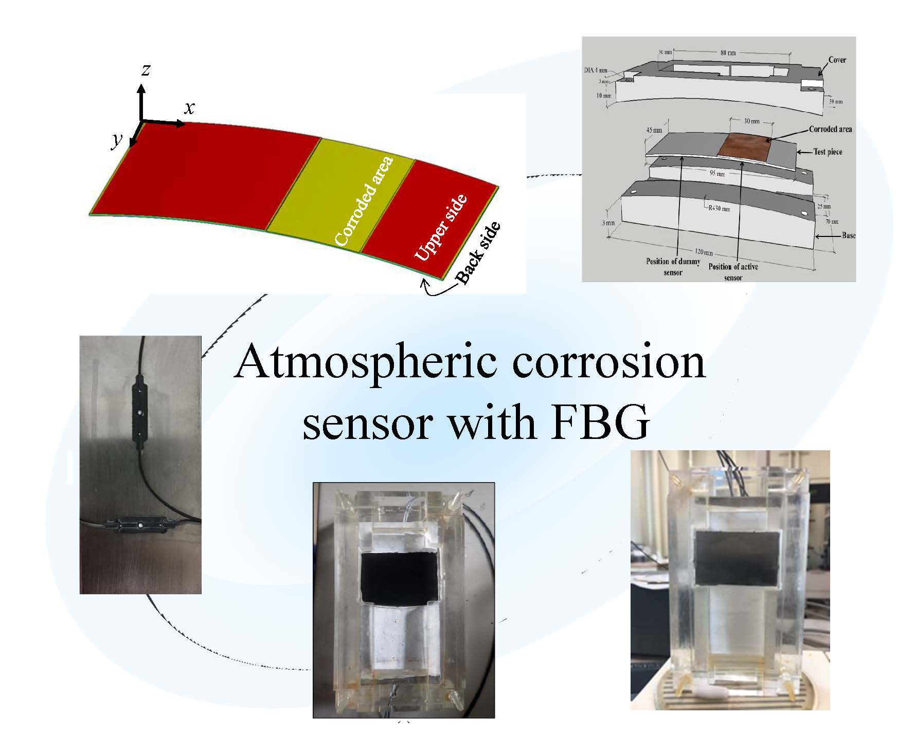
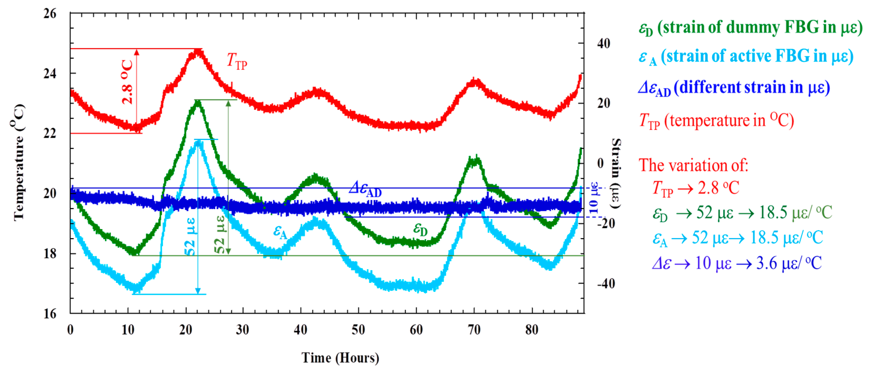
2.4. Compensation of Thermal Strain

We firstly conducted preliminary experiments to investigate the effect of environmental temperature drift on the strain measured by the FBG sensors of the ACSSM. Strain and temperature reflection spectra were measured with a commercial optical interrogation unit from Micron Optics (optical sensing interrogator, model sm125) for 88 h with a data sampling interval of 1 min, controlled by the ENLIGHT software package. As mentioned above, two os3200 FBG sensors from Micron Optics were used as active and dummy strain sensors and an os4200 FBG sensor was used as a temperature sensor. The data obtained from this test were used for further calibration in subsequent experiments.

2.5. Accelerated Corrosion Using Galvanostatic Electrolysis

We conducted galvanostatic electrolysis experiments to verify the accuracy of our technique in identifying corrosion rates. An illustration of the set-up used in these experiments is shown in Figure 4. We used a 1 mol/L hydrochloric acid solution for accelerated simulation of the effects of environmental corrosion, and a stirrer to ensure a homogeneous liquid mixture. To reduce its thickness, a current of 0.3 A was applied to the test piece, which acted as the working electrode, through the potentiostat/galvanostat. The strain on the test piece was measured using an optical sensing interrogator and personal computer setup sampling at an interval of 30 s. The thickness of the test piece was measured before and after the experiment to verify the change in thickness (Δh) estimated from the strain measurement. Finally, the working electrode and counter electrode were constructed from the same material.

3. Result

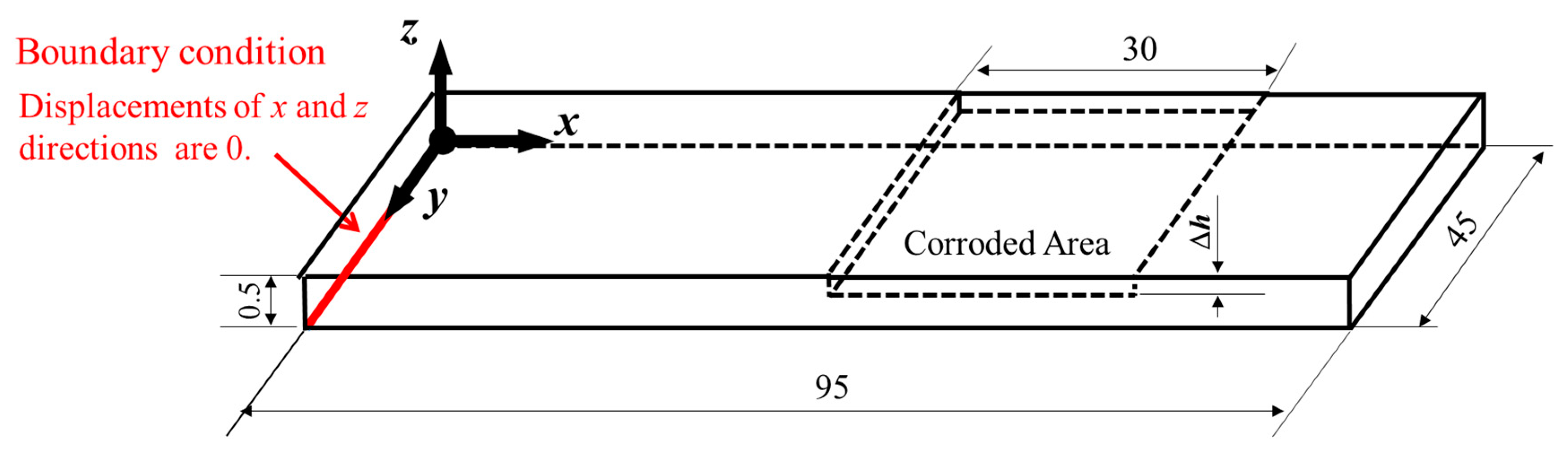
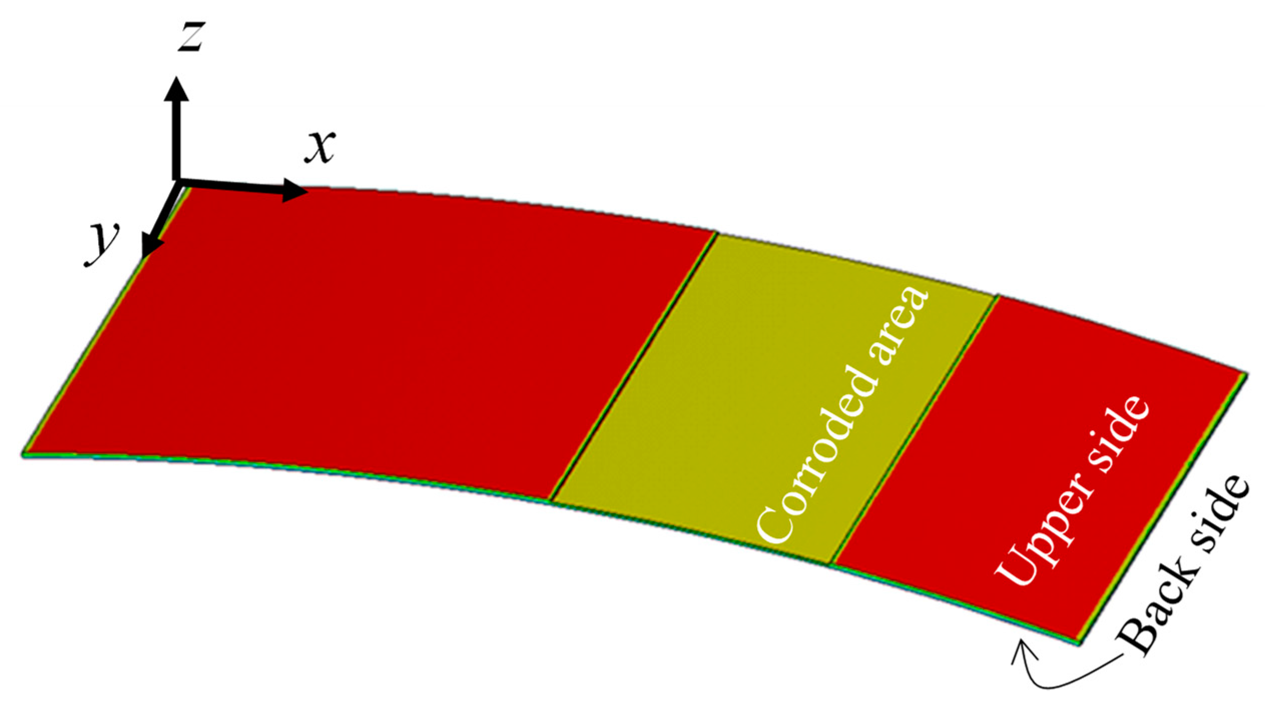
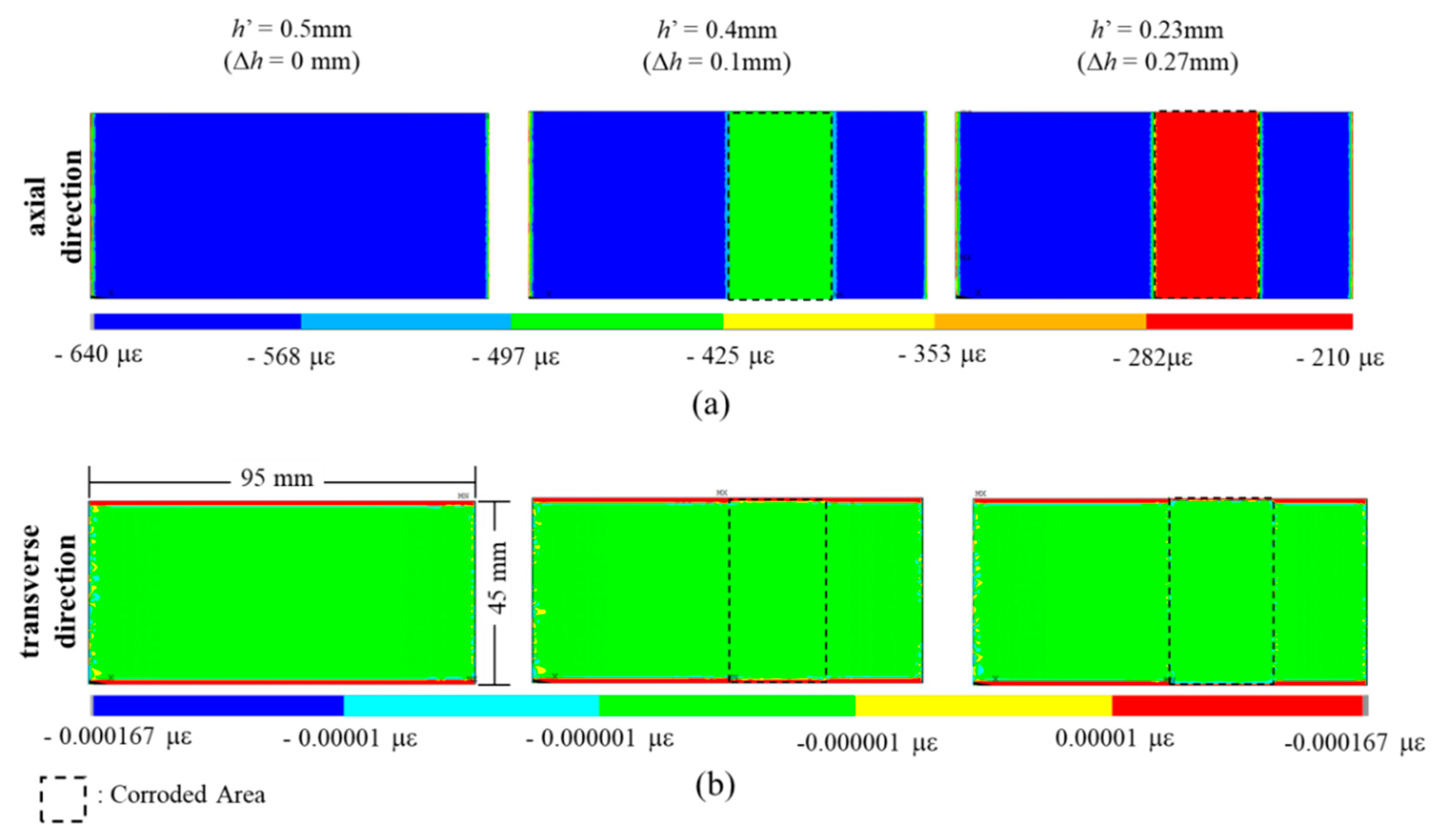
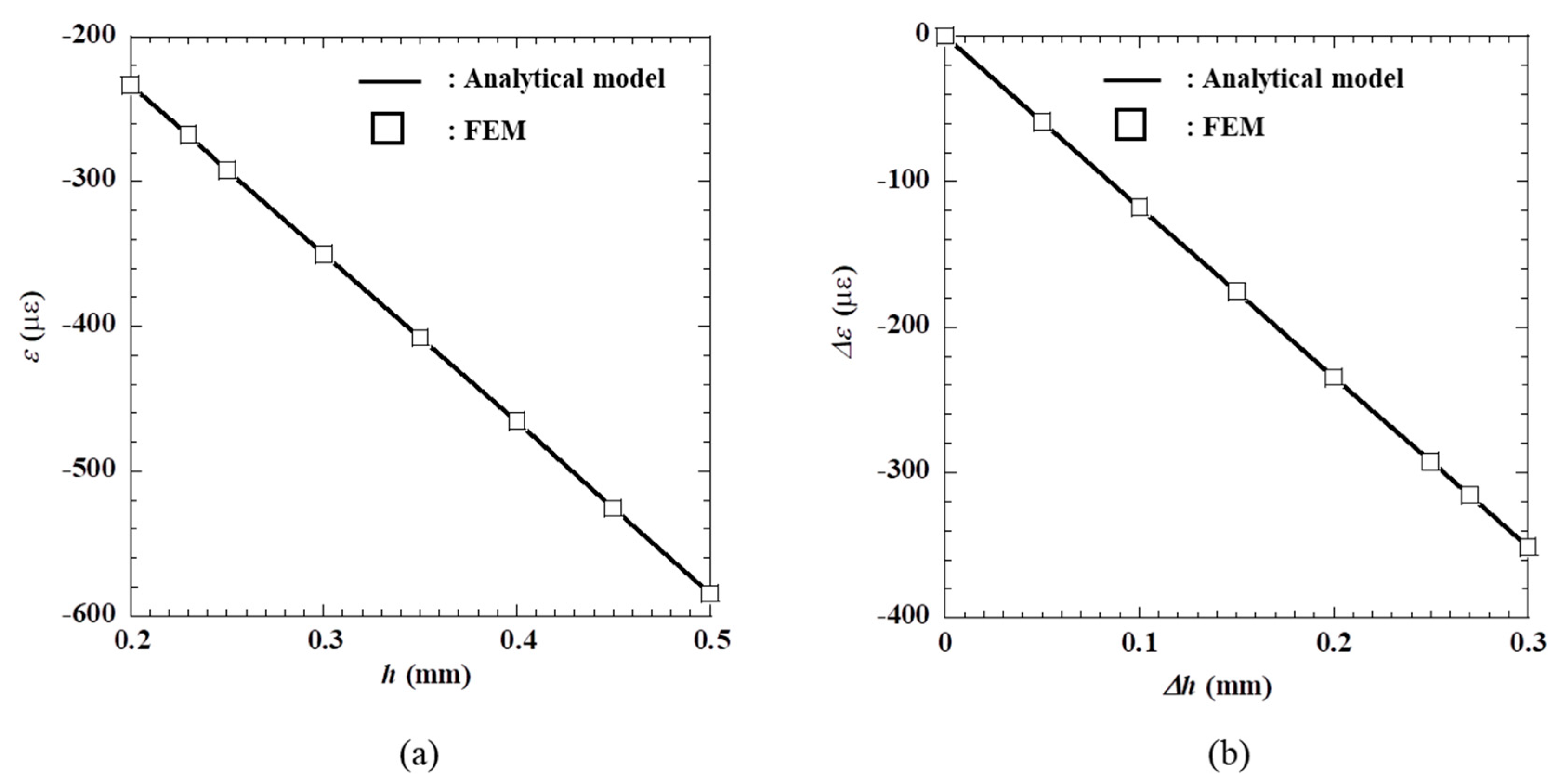
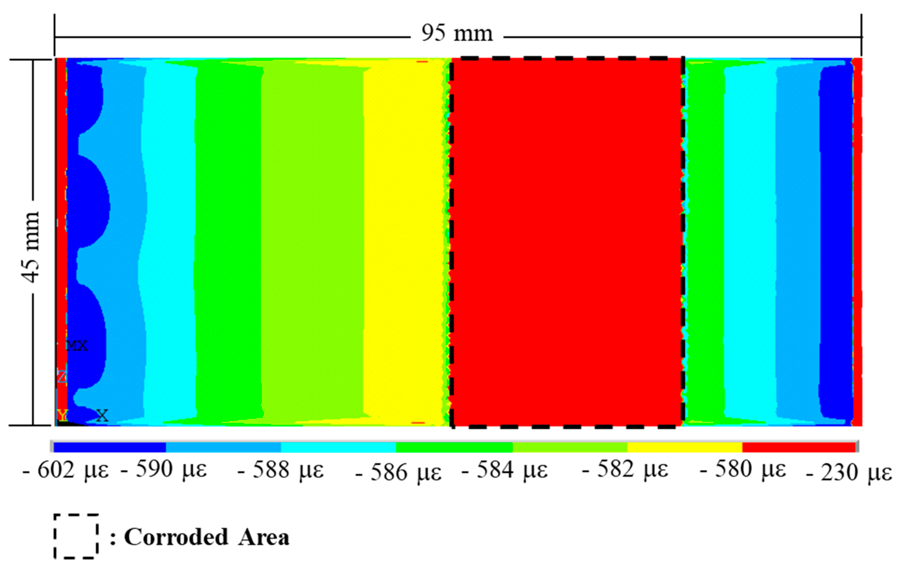
3.1. Numerical Analysis

To isolate components of strain resulting from reduced test piece thickness due to corrosion from components resulting from deviations to the experimental environment, accurate configuration of the positions of the active and dummy FBG sensors is necessary. To determine these positions, we analyzed the behavior of the low-carbon steel test pieces subject to various sources of strain with FEM, using a commercial software (ANSYS Mechanical APDL 18.2 from ANSYS Inc., (Canonsburg, PA, USA). Figure 5 shows the analytical geometry and boundary conditions applied to the test piece before applying ρ of 430 mm to the test piece. The z displacement along the y-axis at the x = 0 node of the test piece was fixed to 0 before/after applying ρ of 430 mm to the test piece. After applying ρ of 430 mm to the test piece, the z coordinates of the test piece at each x coordinates were determined according to the equation below:

$$z=-430+2.6315-\sqrt{{430}^2-{(x-47.5)}^2}$$

(10)

The geometry of the experimental apparatus indicates that the back side of the test piece experiences a compressive strain, while the surface of the piece experiences a tensile strain (Figure 1). Figure 6 shows the analytical result with a thickness reduction of 0.2 mm. Red and yellow colors mean 581 με and 350 με in axial direction. The dimension is 95 mm in length and 45 mm in width and the corroded area is 1350 mm² (30 mm × 45 mm). Figure 7 shows the side view of the xy plane of simulated strain distribution on the back side of the test piece with and without a reduction to the thickness of the corroded area, with Figure 7a depicting the distribution in the axial direction, and Figure 7b depicting the distribution in the transverse direction. Without a reduction in thickness (h = 0.5 mm), a uniform strain (as indicated by the homogenous blue shading) of −579 µε was calculated in the axial direction from an average of five points, a value which is similar to the one predicted by analytical methods (−581 µε). In contrast, in the transverse direction, the strain was 0 µε, indicating that the moment applied a longitudinal strain in the x direction of the test piece. Similarly, for the corroded area of the test piece, when h = 0.1 mm and h = 0.27 mm, the magnitude of the strain in the axial direction predicted using numerical and analytical models was the same. Based on these FEM simulations, a decrease in the thickness of the corroded area of the test piece does not affect the strain distribution in the transverse direction.

The relationship between the longitudinal strain and the thickness of the test piece is shown in Figure 8; Figure 8a shows the relationship between the absolute strain in the x direction and the thickness of the test piece, while Figure 8b shows the relationship between the change in strain (∆ε) and change in thickness (∆h). We note a linear relationship between these two parameters, as suggested by (2), and good correlation between the analytical results and the finite element simulation, indicating that the operating principle of the atmospheric corrosion sensor is reasonable.

A summary of the results of FEM simulations (conducted at a base temperature of 300 K and an elevated temperature of 310 K) is given in

Table 1. Strains obtained from FEM simulation.

h [mm]	Δh [mm]	Strain (με)
		Corroded Area					Uncorroded Area
		Axial Direction					Axial Direction			Transverse Direction
		${\mathit{\epsilon }}_{\Delta \mathit{h}}^{\mathbf{C}}\mathbf{at}300\mathbf{K}$	εC at 300 K	${\mathit{\epsilon }}_{\Delta \mathit{h}}^{\mathbf{C}}\mathbf{at}310\mathbf{K}$	ΔεC at 310 K	$\Delta {\mathit{\epsilon }}_{\Delta \mathit{T}=10\mathbf{K}}^{\mathbf{C}}$	ΔεUC at 300 K	ΔεUC at 310 K	$\Delta {\mathit{\epsilon }}_{\Delta \mathit{T}=10\mathbf{K}}^{\mathbf{UC}}$	ΔεUC at 300 K	ΔεUC at 310 K	$\Delta {\mathit{\epsilon }}_{\Delta \mathit{T}=10\mathbf{K}}^{\mathbf{UC}}$
0.5	0	−584	0	−467	0	117	−584	−467	117	0	117	117
0.45	0.05	−525	59	−408	59	117	-
0.4	0.1	−466	118	−349	118	117
0.35	0.15	−408	176	−291	176	117
0.3	0.2	−350	234	−233	234	117
0.25	0.25	−292	292	−175	292	117
0.23	0.27	−268	316	−151	316	117
0.2	0.3	−233	351	−116	351	117

. Here, we have included the strain in the axial direction in the corroded area (ε^C) where the active FBG sensor was set up, and the strain in the axial and transverse directions under the uncorroded area (ε^UC) where the dummy FBG was set up. Δε^C was obtained from the strain after thickness reduction (${\epsilon }_{\Delta \mathrm{h}}^{\mathrm{C}}-{\epsilon }_{\Delta \mathrm{h}=0}^{\mathrm{C}}$). When ΔT = 10 K, the strain changed by 117 με in both the axial and transverse directions, corresponding to a uniform thermal expansion of 11.7 με/K. The results indicate that the thermal strain in the corroded and uncorroded areas is the same, in both the axial and transverse directions.

By using Equations (7)–(9), ε_A, ε_D, and Δε_AD can be written as follows:

$${\epsilon }_{\mathrm{A}}=\Delta {\epsilon }^{\mathrm{C}}-\Delta {\epsilon }_{\Delta T}^{\mathrm{C}}$$

(11)

$${\epsilon }_{\mathrm{D}}=\Delta {\epsilon }^{\mathrm{UC}}-\Delta {\epsilon }_{\Delta T}^{\mathrm{UC}}$$

(12)

$$\Delta {\epsilon }_{\mathrm{AD}}={\epsilon }_{\mathrm{A}}-{\epsilon }_{\mathrm{D}}=\Delta {\epsilon }^{\mathrm{C}}-\Delta {\epsilon }_{\Delta T}^{\mathrm{C}}-(\Delta {\epsilon }^{\mathrm{UC}}-\Delta {\epsilon }_{\Delta T}^{\mathrm{UC}})$$

(13)

From FEM simulation in Table 1, $\Delta {\epsilon }_{\Delta T}^{\mathrm{C}}=\Delta {\epsilon }_{\Delta T}^{\mathrm{UC}}$ = 117 με for ΔT = 10 K. Thus,

$$\Delta {\epsilon }_{\mathrm{AD}}=\Delta {\epsilon }^{\mathrm{C}}-\Delta {\epsilon }^{\mathrm{UC}}$$

(14)

Δε^C and ${\mathsf{\Delta }\epsilon }_{\mathsf{\Delta }T}^{\mathrm{C}}$ are the differential strains in the corroded area which correspond with the first and second term in Equation (7), respectively. Δε^UC and ${\mathsf{\Delta }\epsilon }_{\mathsf{\Delta }T}^{\mathrm{UC}}$ are the difference strains in the uncorroded area which correspond with the first and second term in Equation (8). Δε_AD is the purposed signal which has relation with the thickness reduction of the test piece, as shown in Equation (2). We used this parameter for the experimental parameter as describes in the Results and Discussion sections.

The side view of the xy plane of the magnified strain distribution in the axial direction of a test piece with a thickness reduction of 0.27 mm is shown in Figure 9. We note a 350 με difference between the strain at the edge and the center of the corroded area. More importantly, the strain is not uniform in the uncorroded area; a difference of approximately 12 με can be observed. This non-uniform strain affects accurate estimation of the reduction in the thickness of the test piece, since the changes to be measured are very small. Hence, we set up the dummy FBG sensor in the y direction of the uncorroded area, as the strain due to environmental factors is identical in both directions, explaining the configuration of the active and dummy FBG sensors on the test piece shown in Figure 3.

3.2. Thermal Strain Compensation

Figure 10 shows the results of the thermal strain measured by the FBG sensors of the ACSSM in the preliminary experiments. In this figure, T_TP is the temperature of the test piece in degrees centigrade, ε_A is the strain from the active FBG sensor in με, ε_Δ is the strain from the dummy FBG sensor in με, and Δε_AD is the difference in strain between ε_A and ε_D. Both sensors had similar responses to temperature variations, producing a maximum change in strain of approximately 52 με for a 2.8 °C temperature variation, in the absence of changes to the thickness of the test piece. In contrast, for the same variation in temperature, the maximum change in the value of Δε_AD was ~10 με. This reduced sensitivity to temperature makes this signal more suitable for strain measurement to determine the atmospheric corrosion rate, which requires high resolution and long-term data monitoring in the field.

3.3. Galvano-Static Electrolysis Experiment

Figure 11 shows the results of the galvanostatic electrolysis experiment, with the light blue line representing the output of the active strain sensor (ε_A), the green line representing the output of the dummy strain sensor (ε_D), and the red line representing the output of the temperature sensor (T_Tp). All three sensors produced a similar output before the current was applied from the potensiostat/galvanostat. In contrast, on the application of the current, a linear increase in the strain signal could be observed during electrolysis using ε_A. ε_D and T_Tp exhibit a similar behavior. The strain signals remain fairly static, with both sensors indicating that the electrolysis process does not result in extreme temperature changes. The dark blue line in this figure is Δε_AD, which exhibits a similar trend to ε_A.

4. Discussion

A figure of the test piece following the experiment is shown in Figure 12a, which depicts the effects of electrolysis on the apparatus. To evaluate the accuracy of the active–dummy FBG sensors’ estimation of changes in thickness, we measured the actual thickness and weight of the test piece before and after electrolysis. The labeled points in Figure 12b were measured using a micrometer, and the thickness of the test piece was determined based on the average of these measurements. The average values calculated before and after corrosion were 0.48 mm and 0.36 mm, respectively, corresponding to a change in thickness (Δh_T) of 0.12 mm. To estimate change in thickness using the weight of the test piece, we evaluated the equation below:

$$\Delta h_W=\frac{\Delta W}{S d}$$

(15)

where ΔW is the change in weight, S is the area of the corroded region (1350 mm²), and d is the density of the test piece (0.0078 g⋅mm⁻³). The test piece was weighed at 16.0 g and 14.6 g before and after the experiment, respectively. Hence, ΔW = 1.4 g, and from Equation (15), Δh_W = 0.132 mm. The final value of Δε_AD obtained in the electrolysis experiment was 143 με, indicating that Δh = 0.12 mm, according to (2). A comparison of these results is given in

Table 2. Comparison of thickness reduction measured by thickness and weight loss.

	Based on Strain Measurement (Δh)	Based on Actual Thickness (ΔhT)	Based on Weight Loss (ΔhW)
Thickness (μm)	123	120	132
Difference (%)	-	2.5	6.8

. A maximum difference in thickness of 6.8% was noted, highlighting that the modifications have improved the performance of the ACSSM, which produced a difference of 12% in previous experiments.

5. Conclusions

In this study, we proposed an improvement to the ACSSM technique, replacing conventional strain gauges with active–dummy FBG sensors. The orthogonal configuration of active–dummy FBG sensors on the test piece was determined from FEM analysis of the thermal expansion and the reduction in the thickness of the test piece. We observed that Δε, the difference between the outputs of the active and the dummy FBG sensors, is less sensitive to changes to the experimental environment, enabling the collection of more accurate and constant signals less affected by temperature drift during prolonged measurement. Results of galvanostatic electrolysis experiments indicated an approximate difference of 6.8% between thicknesses estimated using the strain measured with the active–dummy FBG sensors and that estimated from weight loss, and 2.5% for actual thicknesses measured using a digital micrometer. These small differences suggest that Δε can be used to determine the atmospheric corrosion rate, which requires high resolution in the field. This quality, in addition to the ability to perform long-term data monitoring, makes the ACSSM with FBG sensors suitable for estimating the atmospheric corrosion of steel structures. Monitoring a test piece with the ACSSM that is fabricated from the same material as the steel structure and exposed to the same environment will contribute to effective decision-making for the maintenance of the steel structure.

References

1. Cai, H.T.; Faisal, R.M.A.; Yu, G.S.; Boon, K.Y. Non-destructive fiber Bragg grating based sensing system: Early corrosion detection for structural health monitoring. Sens. Act. A Phys. 2017, 268, 61–67. [Google Scholar]
2. Muhammad, R.; Syarizal, F.; Syifaul, H.; Juendri, S.; Ahmad, K.A. Atmospheric corrosion of structural steels exposed in the 2004 tsunami-affected areas of Aceh. Int. J. Automot. Mech. Eng. 2013, 7, 1014–1022. [Google Scholar] [CrossRef]
3. Tadashi, S.; Akira, T.; To, D. Atmospheric corrosion behaviours of steels in Japan. Zair. Kank. 2016, C-111, 285–288. [Google Scholar]
4. Isao, S.; Ayaka, O.; Masayuki, I.; Kunihiro, W.; Yafusumi, A. Screen printed atmospheric corrosion monitoring sensor based on electrochemical impedance spectroscopy. Sens. Actuators B Chem. 2009, 139, 292–297. [Google Scholar] [CrossRef]
5. Chungling, L.; Yuantai, M.; Ying, L.; Fuhui, W. EIS monitoring study of atmospheric corrosion under variable relative humidity. Cor. Sci. 2010, 52, 3677–3686. [Google Scholar] [CrossRef]
6. Naoya, K.; Masatoshi, H.; Toshirou, Y.; Hiroshi, K.; Kazumi, M.; Yukihisa, K.; Shinji, O. Atmospheric corrosion sensor based on strain measurement. Meas. Sci. Technol. 2016, 28, 015106. [Google Scholar]
7. Nining, P.; Naoya, K.; Shinji, O.; Hiroshi, K. Development of amplifier circuit by active dummy method for atmospheric corrosion monitoring in steel based on strain measurement. Metals 2018, 8, 5. [Google Scholar]
8. Nining, P.; Naoya, K.; Shinji, O.; Hiroshi, K.; Yukihisa, K. Atmospheric Corrosion Sensor Based on Strain Measurement with an Active Dummy Circuit Method in Experiment with Corrosion Products. Metal 2019, 9, 579. [Google Scholar]
9. Sascha, L.; Philipp, L.; Mario, W.; Katerina, K.; Monika, S.; Elke, T.; Heike, M.; Berhane, G.; Johannes, C.M. Polymer Optical Fiber Sensors for Distributed Strain Measurement and Application in Structural Health Monitoring. IEEE Sens. J. 2009, 9, 1330–1338. [Google Scholar]
10. Drake, D.A.; Sullivan, R.W.; Wilson, J.C. Distributed Strain Sensing from Different Optical Fiber. Inventions 2018, 3, 67. [Google Scholar] [CrossRef] [Green Version]
11. Libo, Y.; Jun, Y.; Limin, Z.; Wei, J.; Xiaoli, D. Low-coherence Michelson interferometric fiber-optic multiplexed strain sensor array: A minimum configuration. Appl. Opt. 2004, 43, 3211–3216. [Google Scholar] [CrossRef]
12. Kamal, R.; Ajay, S. Strain Measurement with Fiber Mach-Zehnder Interferometer Using Spatial Phase Measurement Techniques. Int. J. Sci. Tech. Res. 2019, 8, 1617–1622. [Google Scholar]
13. Genda, C.; Hai, X.; Ying, H.; Zhi, Z.; Yinan, Z. A Novel Long-Period Fiber Grating Optical Sensor for Large Strain Measurement. Proc. SPIE 2009, 7292, 12. [Google Scholar] [CrossRef]
14. Jian, N.W.; Jaw, L.T. Feasibility of Fiber Bragg Grating and Long-Period Fiber Grating Sensors under Different Environmental Conditions. Sensors 2010, 10, 10105–10127. [Google Scholar] [CrossRef]
15. Carlos, R.; Filipe, C.; Carlos, F.; Joaqium, F. FBG based strain monitoring in the rehabilitation of a centenary metallic bridge. Eng. Struct. 2012, 44, 281–290. [Google Scholar]
16. Sherif, Y.; Taha, L.; Mohamed, H.; Mohammad, H. Monitoring of strain induced by heat of hydration, cyclic and dynamic loads in concrete structures using fiber-optics sensors. Measurement 2014, 52, 33–46. [Google Scholar]
17. Li, H.N.; Ren, L.; Li, D.S.; Yi, T.H. Design and Applications of Fiber BRAGG Grating Sensors for Structural Health Monitoring. In Proceedings of the 2013 World Congress on Advances in Structural Engineering and Mechanics (ASEM13), Jeju, Korea, 8–12 September 2013; pp. 2215–2221. [Google Scholar]
18. Hong-lin, L.; Zheng-wei, Z.; Yong, Z.; Bang, L.; Feng, X. Experimental study on an FBG strain sensor. Opt. Fiber Tech. 2018, 40, 144–151. [Google Scholar]
19. Hideaki, M.; Kohei, O.; Nozomi, K.; Kazura, K.; Hirotaka, I. Strain monitoring and defect detection in welded joints by using fiber-optic distributed sensors with high spatial resolution. E-J. Adv. Maintenance 2011, 2, 191–199. [Google Scholar]
20. Michael, C.E.; Sunny, K.; Stefano, T.; Kotekar, P.M.; Richards, W.L.; Gregory, P.C. Strain measurement validation of embedded fiber bragg gratings. Int. J. Optomech. 2010, 4, 22–33. [Google Scholar]
21. Wenbin, H.; Likang, D.; Cheng, Z.; Donglai, G.; Yinquan, Y.; Ning, M.; Wei, C. Optical fiber polarizer with Fe-C film for corrosion monitoring. IEEE Sens. J. 2017, 17, 6904–6910. [Google Scholar]
22. Wenbin, H.; Hanli, C.; Minghong, Y.; Xinglin, T.; Ciming, Z.; Wei, C. Fe-C-coated fibre Bragg grating sensor for steel corrosion monitoring. Cor. Sci. 2011, 53, 1933–1938. [Google Scholar]
23. Ning, Z.; Wei, C.; Xing, Z.; Wenbin, H.; Min, G. Optical sensor for steel corrosion monitoring based on etched fiber bragg grating sputtered with iron film. IEEE Sens. J. 2015, 15, 3551–3556. [Google Scholar]
24. Rosdi, H.; Muhammad, H.A.B.; Katrina, D.; Faisal, R.M.A. Optical-based sensors for monitoring corrosion of reinforcement rebar via an etched cladding Bragg grating. Sensors 2012, 12, 15820–15826. [Google Scholar]
25. Omar, A.; Hwa, K.C.; Muhammad, R.I.; Kok-Sing, L.; Chee, G.T. Monitoring corrosion process of reinforced concrete structure using FBG strain sensor. IEEE Trans. Instrum. Meas. 2017, 66, 2148–2155. [Google Scholar]
26. Simon, K.T.G.; Su, E.T.; Basheer, P.A.; Muhammed, B.; Tong, S.; Kenneth, T.V.G. Monitoring of corrosion in structural reinforcing bars: Performance comparison using in situ fiber-optic and electric Wire Strain Gauge Systems. IEEE Sens. J. 2009, 9, 1494–1502. [Google Scholar]
27. Wen, C.; Dong, X. Modification of the wavelength-strain coefficient of FBG for the prediction of steel bar corrosion embedded in concrete. Opt. Fib. Tech. 2012, 18, 47–50. [Google Scholar]
28. Khalil, A.H.; Nader, V.; Paul, R.; Lydia, L.; Oleg, S. Strain based FBG sensor for real-time corrosion rate monitoring in pre-stressed structures. Sens. Act. B Chem. 2016, 236, 276–285. [Google Scholar]
29. Marcelo, M.W.; Regina, C.S.B.A.; Bessie, A.R.; Fabio, V.B.D.N. A Guide to Fiber Bragg Grating Sensors. Intech 2013, 24. [Google Scholar] [CrossRef] [Green Version]
30. Jigou, L.; Cornelia, S.H.; Gunter, B. Dynamic strain measurement with a fibre Bragg grating sensor system. Measurement 2002, 32, 151–161. [Google Scholar]
31. Hang-yin, L.; Kin-tak, L.; Li, C.; Wei, J. Viability of using an embedded FBG sensor in a composite structure for dynamic strain measurement. Measurement 2006, 39, 328–334. [Google Scholar]
32. Rosa, A.P.H.; Ricardo, M.A.; Susana, F.S.; Martin, B.; Kay, S.; Jens, K.; Manuel, L.A.; Jose, L.S.; Orlanclo, F. Simultaneous measurement of strain and temperature based on clover microstructured fiber loop mirror. Measurement 2015, 65, 50–53. [Google Scholar]
33. Jianping, H.; Zhi, Z.; Jinping, O. Simultaneous measurement of strain and temperature using a hybrid local and distributed optical fiber sensing system. Measurement 2014, 47, 698–706. [Google Scholar]
Figure 1. Illustration of (a) a non-corroded test piece, and (b) a corroded test piece highlighting the geometry of the normal and bending positions.
Metals 10 01076 g001
Figure 2. Diagram of the atmospheric corrosion sensor based on strain measurement (ACSSM) apparatus, consisting of a base, the test piece, and a cover.
Metals 10 01076 g002
Figure 3. Configuration of active and dummy fiber Bragg grating (FBG) sensor on the (a) front side and (b) back side of the test piece. (c) The actual figure of the FBG sensors attached to the test piece. The unit is in mm.
Metals 10 01076 g003
Figure 4. Set-up of galvanostatic electrolysis experiments to reduce thickness of the test piece.
Metals 10 01076 g004
Figure 5. Model of the test piece and boundary conditions used in simulation. The unit is in mm.
Metals 10 01076 g005
Figure 6. Analytical result with a thickness reduction of 0.2 mm. Red and yellow colors mean 581 με and 350 με in axial direction. The dimension is 95 mm in length and 45 mm in width and the corroded area is 1350 mm2 (30 mm × 45 mm).
Metals 10 01076 g006
Figure 7. The side view of xy plane of FEM-simulated strain distribution on the back side of the test piece with and without a reduction in thickness, (a) in the axial direction, and (b) in the transverse direction.
Metals 10 01076 g007
Figure 8. (a) Relationship between the strain (ε) and thickness of the test piece (h) from FEM simulations. (b) Relationship between the change in strain (∆ε) and change in thickness Δh in mm from FEM simulations. The analytical model provides the line of best fit in both plots.
Metals 10 01076 g008
Figure 9. The side view of the xy plane of magnified strain distribution on the back side of the test piece in the axial direction, with a 0.27 mm reduction in thickness.
Metals 10 01076 g009
Figure 10. Variation in the sensor signal patterns in the absence of corrosion. Only ΔεAD shows no dependence on temperature.
Metals 10 01076 g010
Figure 11. Strains measured during the electrolysis process. Equivalent strain from the actual change in thickness (ΔhT) and change in thickness evaluated from weight loss (ΔhW) are labeled on the plot for comparison.
Metals 10 01076 g011
Figure 12. (a) Test piece in the experimental apparatus following electrolysis. (b) Location of points measured for evaluation of change in thickness after electrolysis.
Metals 10 01076 g012